Author Contributions
Conceptualisation, T.M. and G.K.; Methodology, T.M.; Software, T.M.; Validation, T.M., D.T.M. and G.K.; Formal Analysis, T.M.; Investigation, T.M.; Resources, T.M.; Data Curation, T.M.; Writing—Original Draft Preparation, T.M.; Writing—Review & Editing, T.M., D.T.M. and G.K.; Visualisation, T.M.; Supervision, D.T.M. and G.K.; Project Administration, T.M.; Funding Acquisition, G.K.
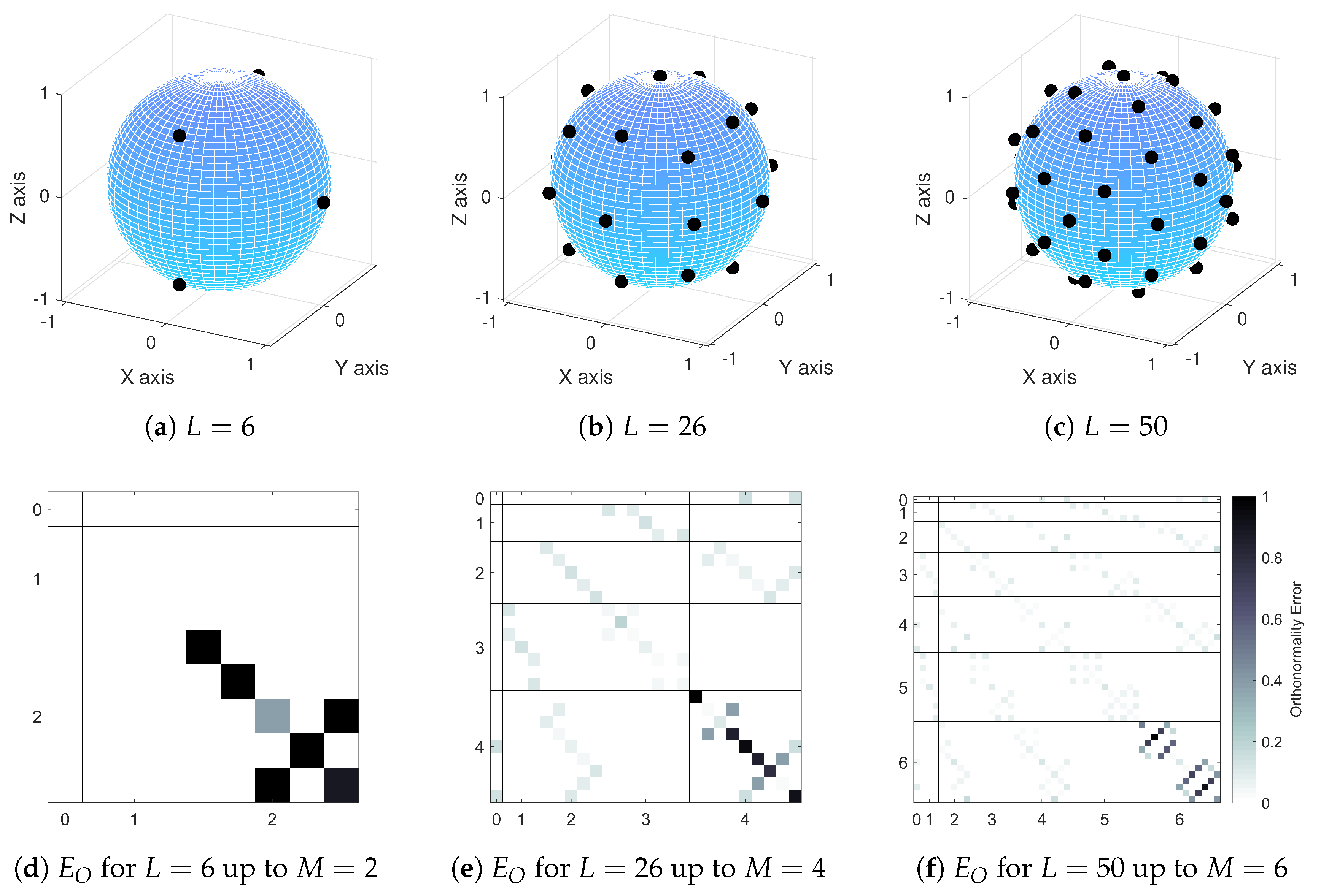
Figure 1.
Loudspeaker layouts and orthonormality error matrices for the three Lebedev loudspeaker configurations used in this paper: (a) loudspeaker layout for (), (b) loudspeaker layout for (), (c) loudspeaker layout for (), (d) orthonormality error matrix plot for (), (e) orthonormality error matrix plot for () and (f) orthonormality error matrix plot for (). In orthonormality error matrix plots, spherical harmonics of different orders are separated to aid visual clarity.
Figure 2.
Example of the high-frequency differences of decoding with and without Max weighting-fifth-order binaural Ambisonic rendering (Neumann KU 100 HRIRs) at () = (0, 0) (left ear).
Figure 2.
Example of the high-frequency differences of decoding with and without Max weighting-fifth-order binaural Ambisonic rendering (Neumann KU 100 HRIRs) at () = (0, 0) (left ear).
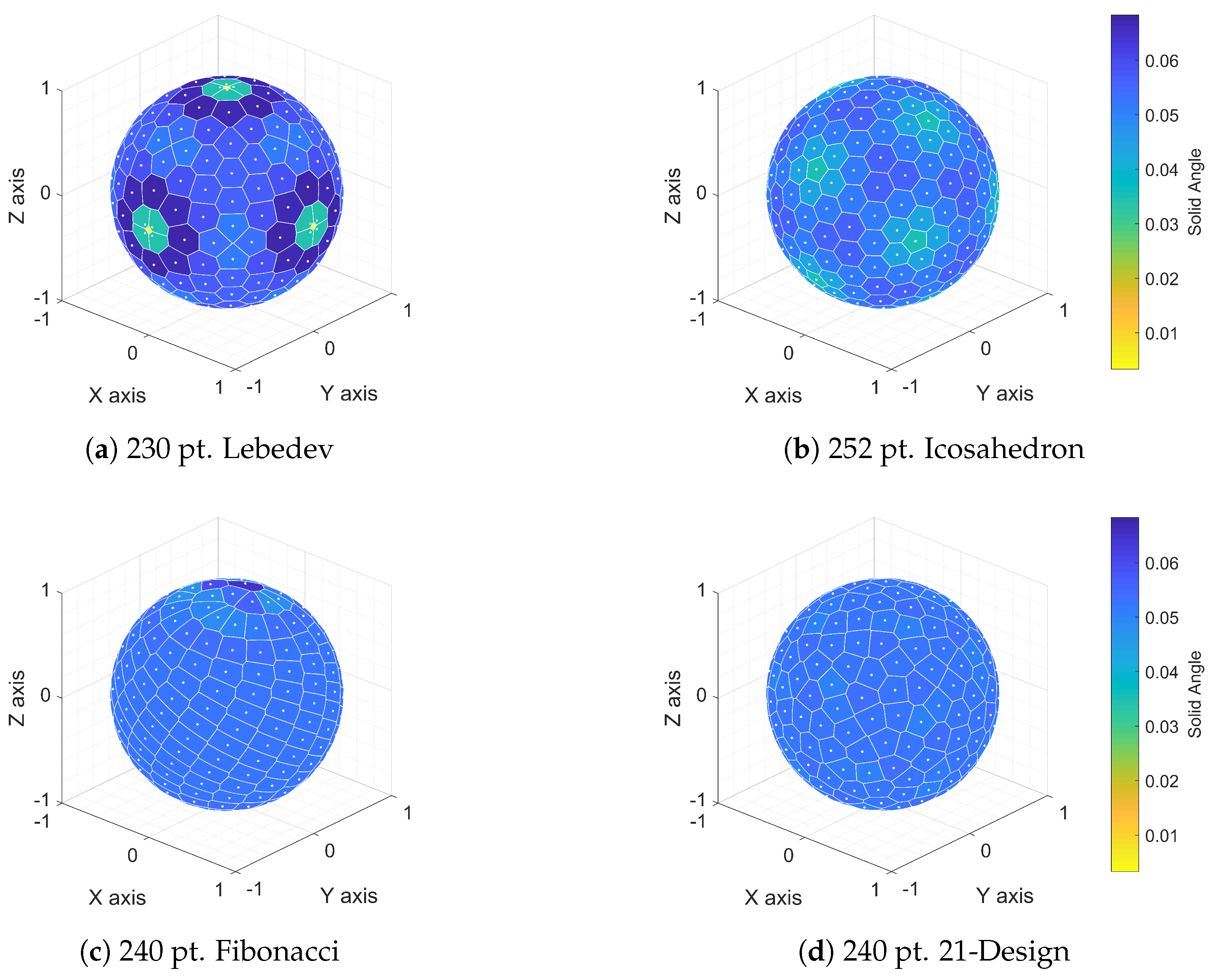
Figure 3.
Voronoi sphere plots demonstrating the regularity in spherical distribution of points for four quadrature methods: (a) 230 pt. Lebedev, (b) 252 pt. Icosahedron, (c) 240 pt. Fibonacci and (d) 240 pt. 21-Design.
Figure 3.
Voronoi sphere plots demonstrating the regularity in spherical distribution of points for four quadrature methods: (a) 230 pt. Lebedev, (b) 252 pt. Icosahedron, (c) 240 pt. Fibonacci and (d) 240 pt. 21-Design.
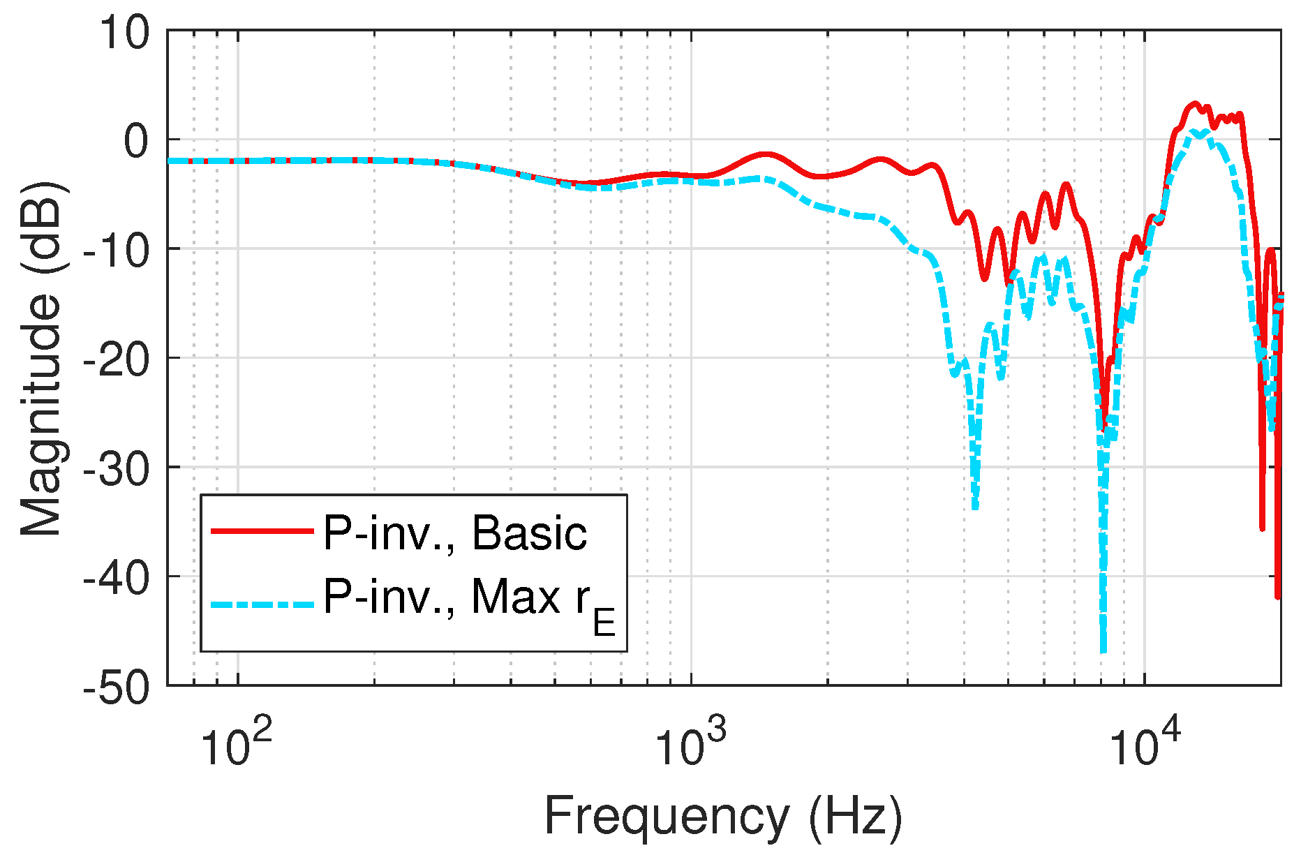
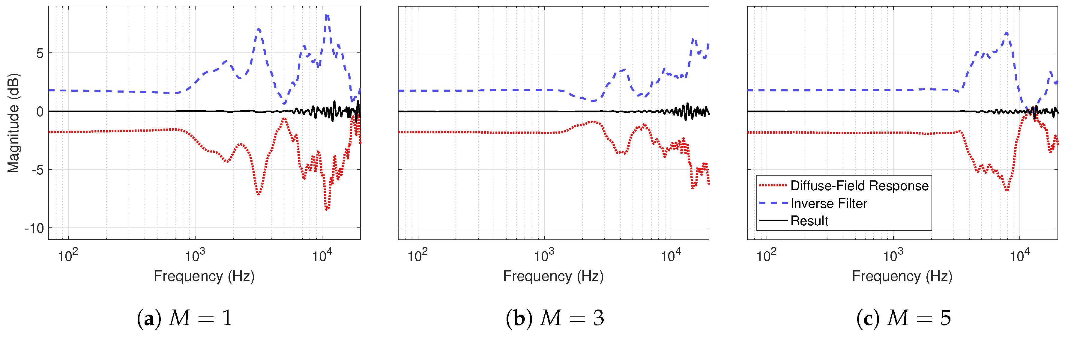
Figure 4.
Diffuse-field response, inverse filters and resulting responses of the three tested Ambisonic configurations (left ear): (a) , (b) and (c) .
Figure 4.
Diffuse-field response, inverse filters and resulting responses of the three tested Ambisonic configurations (left ear): (a) , (b) and (c) .
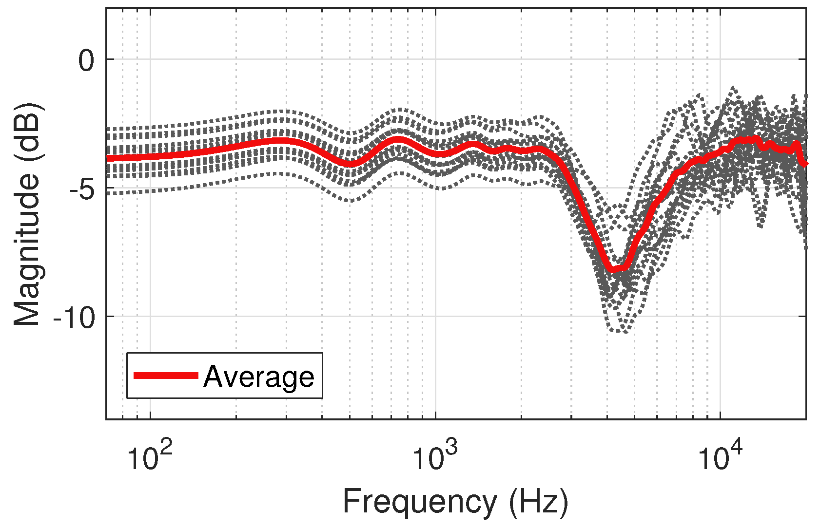
Figure 5.
Diffuse-field responses of the 50 pt. Lebedev loudspeaker configuration for for the 18 human subjects of the SADIE II database, with average response (left ear).
Figure 5.
Diffuse-field responses of the 50 pt. Lebedev loudspeaker configuration for for the 18 human subjects of the SADIE II database, with average response (left ear).
Figure 6.
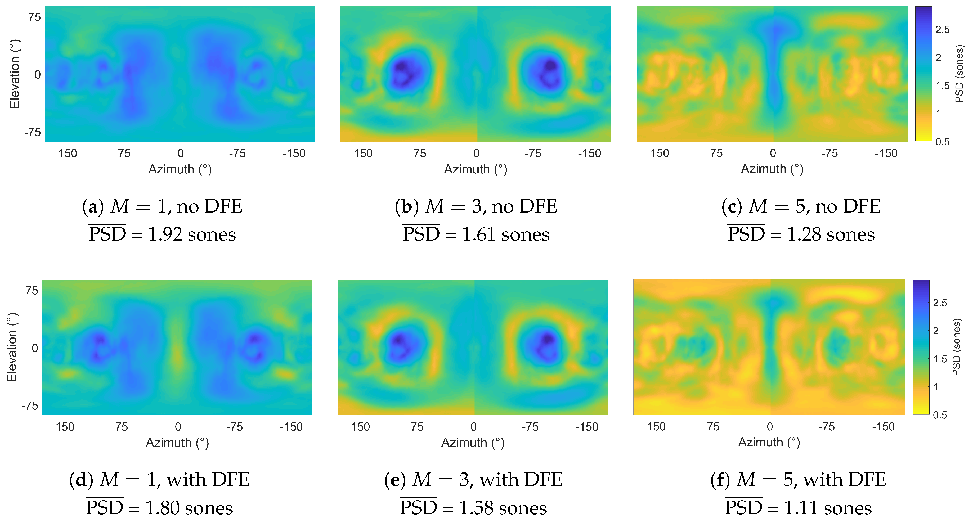
between HRTFs and reference HRTFs with and without DFE (mean of left and right ear PSD calculations): (a) , no DFE, (b) , no DFE, (c) , no DFE, (d) , with DFE, (e) , with DFE and (f) , with DFE. PSD: Perceptual spectral difference; HRTF: Head-related transfer function; DFE: Diffuse-field equalisation.
Figure 6.
between HRTFs and reference HRTFs with and without DFE (mean of left and right ear PSD calculations): (a) , no DFE, (b) , no DFE, (c) , no DFE, (d) , with DFE, (e) , with DFE and (f) , with DFE. PSD: Perceptual spectral difference; HRTF: Head-related transfer function; DFE: Diffuse-field equalisation.
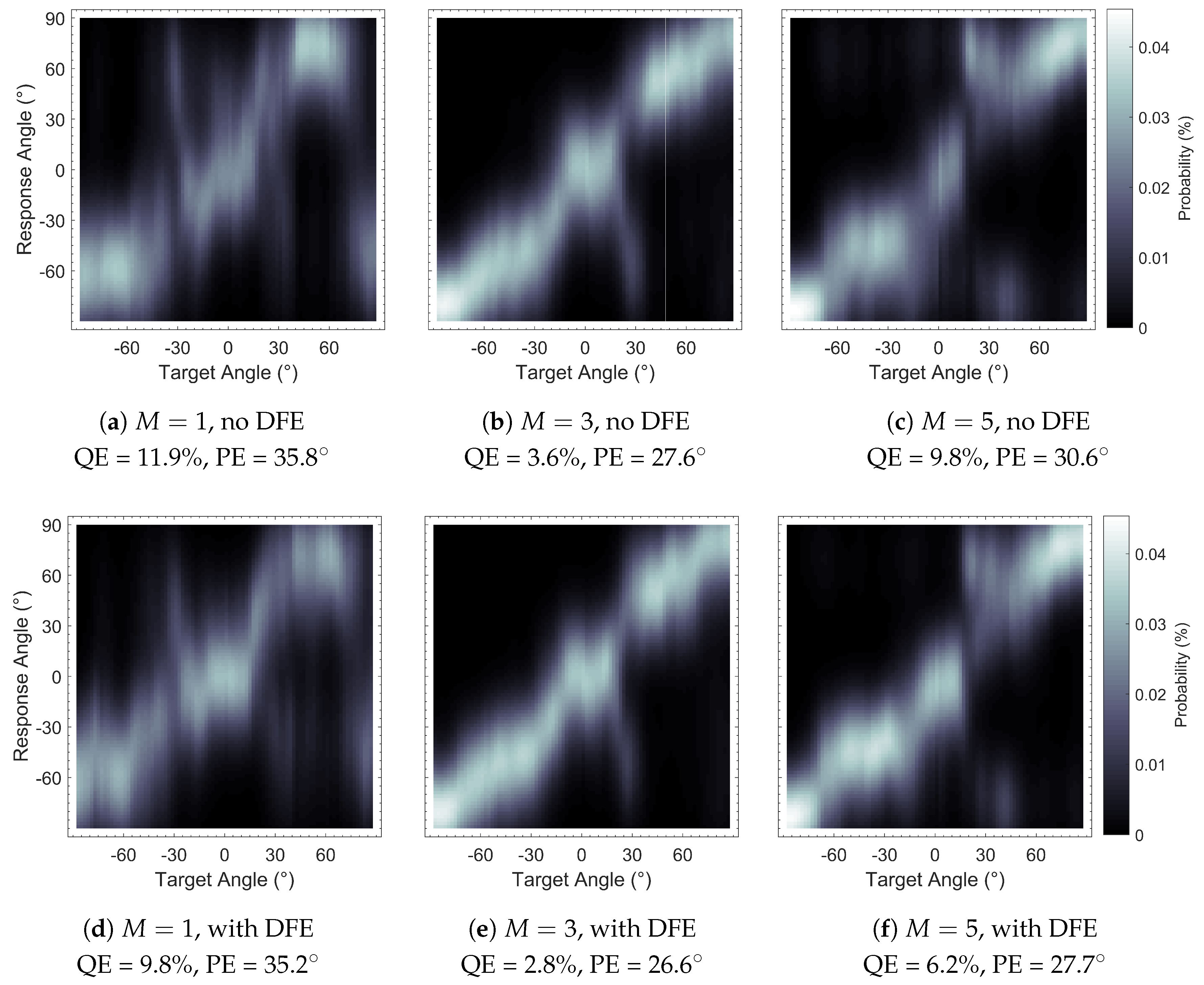
Figure 7.
Sagittal Plane Localisation Model [
44] plots of binaural Ambisonic rendering, with and without Diffuse-Field Equalisation (DFE): (
a)
, no DFE, (
b)
, no DFE, (
c)
, no DFE, (
d)
, with DFE, (
e)
, with DFE and (
f)
, with DFE. Plots show greater clarity (bolder shading) with DFE implementation.
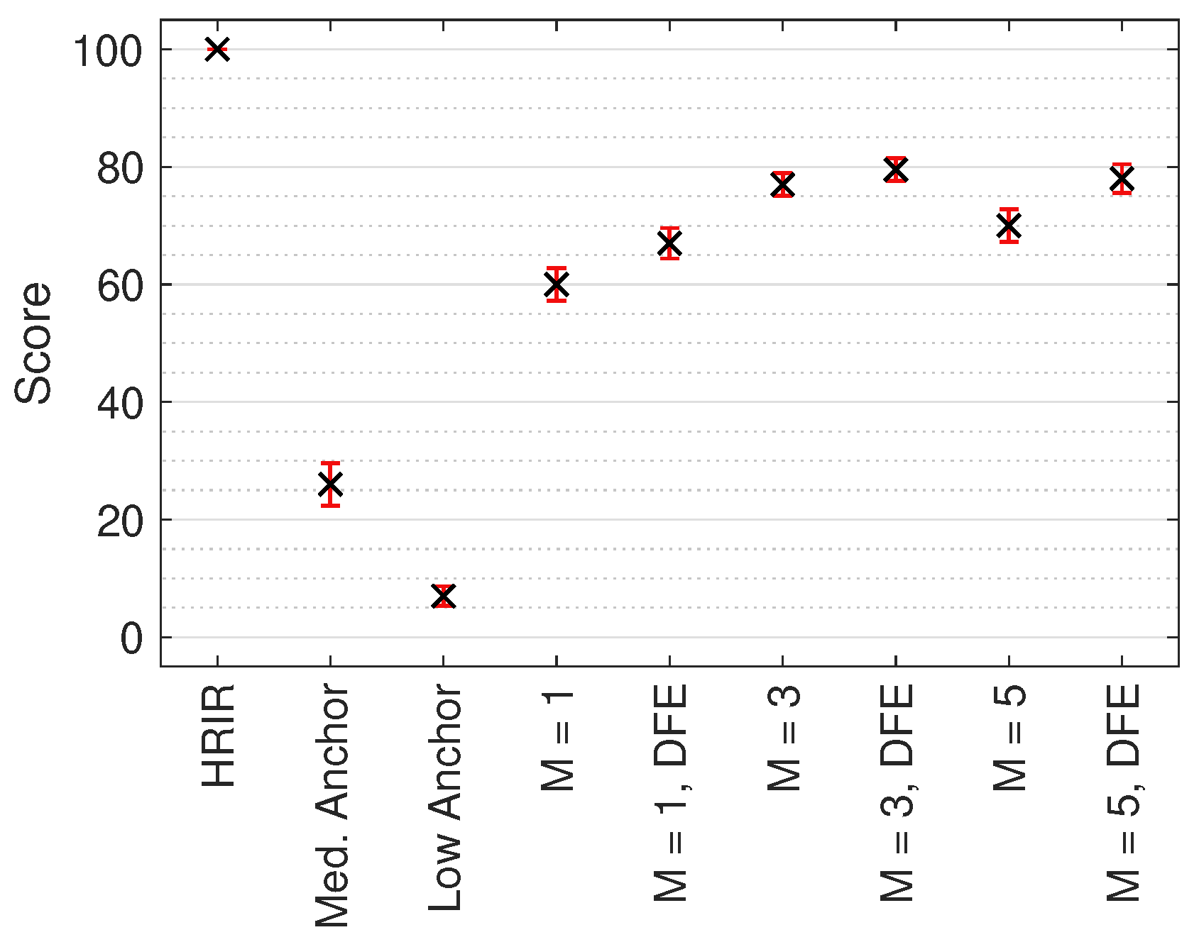
Figure 8.
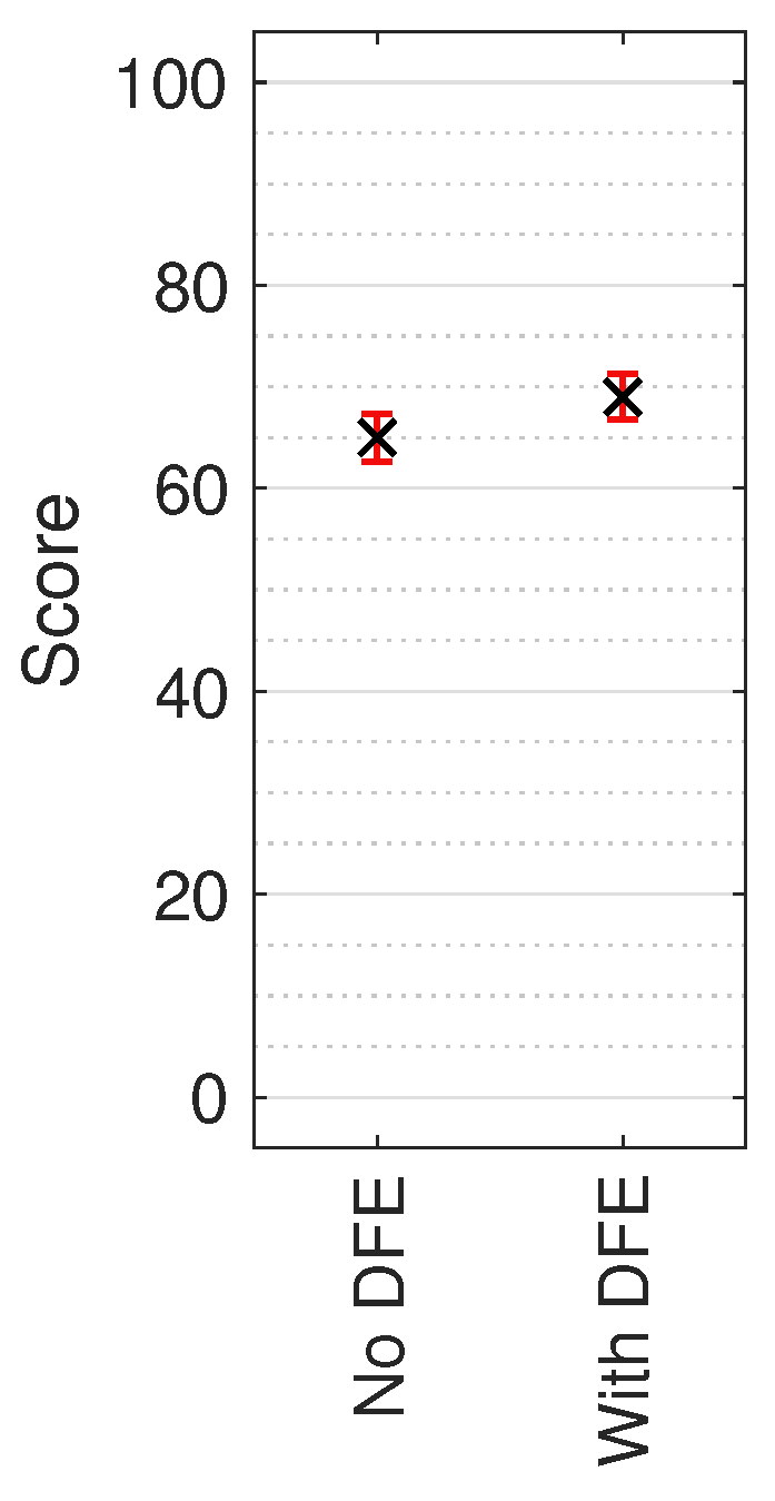
Median MUSHRA results with non-parametric 95% CI across all test sound locations. Score indicates perceived timbral similarity between test stimulus and HRIR reference.
Figure 8.
Median MUSHRA results with non-parametric 95% CI across all test sound locations. Score indicates perceived timbral similarity between test stimulus and HRIR reference.
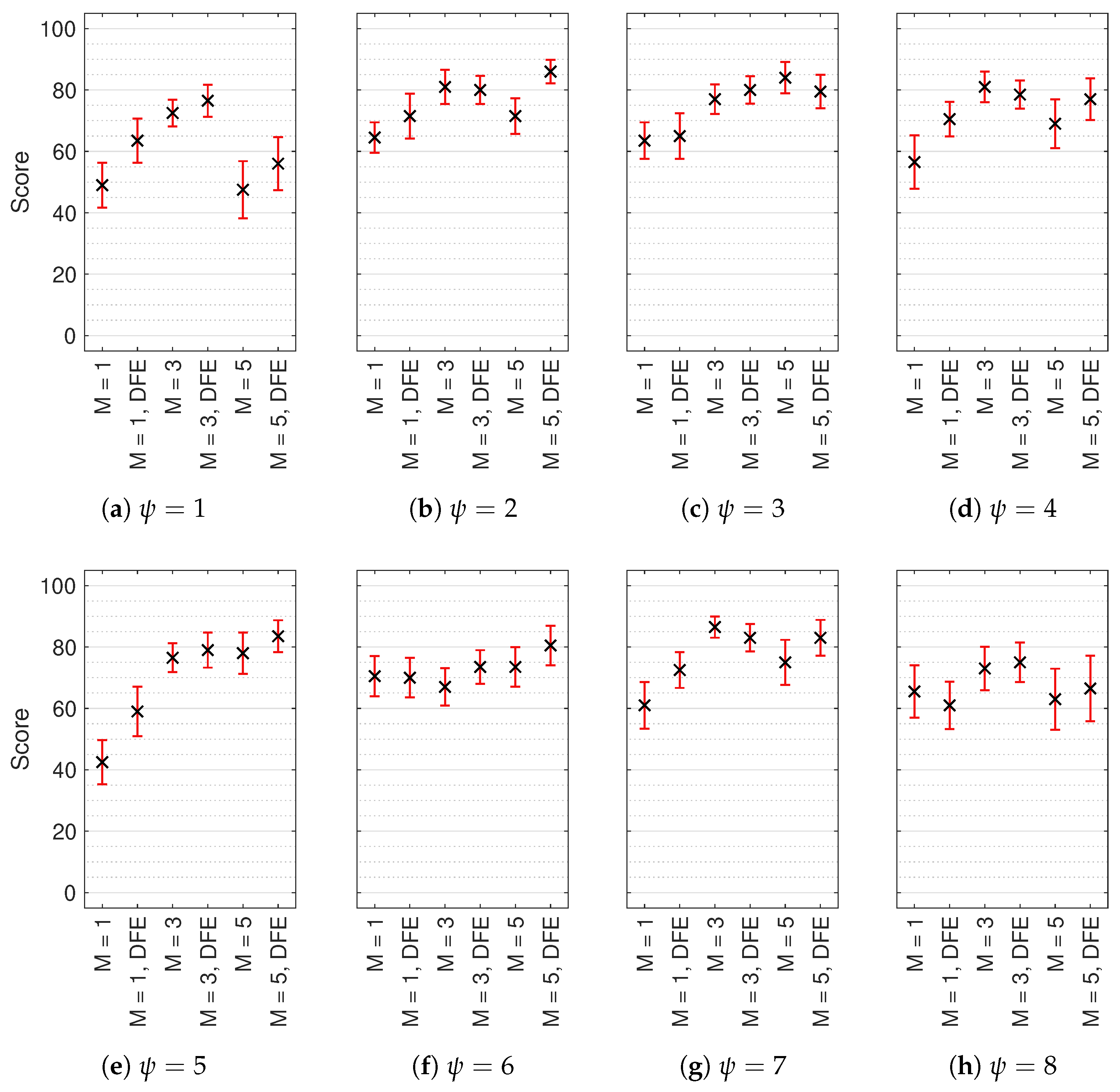
Figure 9.
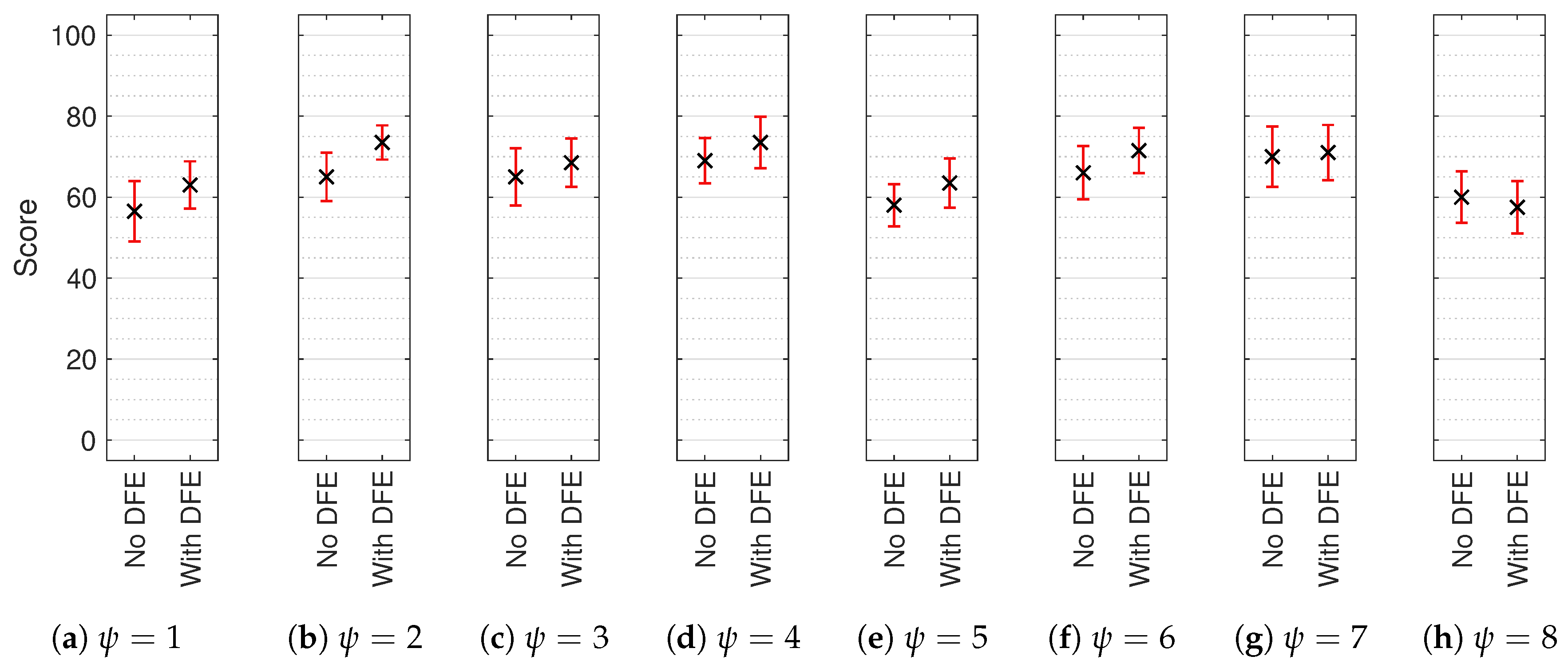
Median multiple stimulus test with hidden reference and anchor (MUSHRA) results with non-parametric 95% confidence intervals (CI) for each test sound location (): (a) , (b) , (c) , (d) , (e) , (f) , (g) and (h) . Reference and anchor scores omitted. Score indicates perceived timbral similarity between test stimulus and HRIR reference.
Figure 9.
Median multiple stimulus test with hidden reference and anchor (MUSHRA) results with non-parametric 95% confidence intervals (CI) for each test sound location (): (a) , (b) , (c) , (d) , (e) , (f) , (g) and (h) . Reference and anchor scores omitted. Score indicates perceived timbral similarity between test stimulus and HRIR reference.
Figure 10.
Median AB results with non-parametric 95% CI across all test sound locations. Score indicates perceived timbral consistency between the three tested orders of Ambisonics.
Figure 10.
Median AB results with non-parametric 95% CI across all test sound locations. Score indicates perceived timbral consistency between the three tested orders of Ambisonics.
Figure 11.
Median AB results with non-parametric 95% CI for each test sound location (): (a) , (b) , (c) , (d) , (e) , (f) , (g) and (h) . Reference and anchor scores omitted. Score indicates perceived timbral consistency between the three tested orders of Ambisonics.
Figure 11.
Median AB results with non-parametric 95% CI for each test sound location (): (a) , (b) , (c) , (d) , (e) , (f) , (g) and (h) . Reference and anchor scores omitted. Score indicates perceived timbral consistency between the three tested orders of Ambisonics.
Table 1.
RMS Max weightings for Ambisonic orders 1 to 5.
Table 1.
RMS Max weightings for Ambisonic orders 1 to 5.
| M | 1 | 2 | 3 | 4 | 5 |
|---|
| 0.707 | 0.633 | 0.600 | 0.581 | 0.569 |
Table 2.
Dual-band decode crossover frequencies producing 20% integrated D-error for Ambisonic orders 1 to 5, according to [
23].
Table 2.
Dual-band decode crossover frequencies producing 20% integrated D-error for Ambisonic orders 1 to 5, according to [
23].
| M | 1 | 2 | 3 | 4 | 5 |
|---|
| f (Hz) | 743 | 1346 | 1960 | 2595 | 3230 |
Table 3.
Solid angle weighted mean values of PSD between reference HRTFs and Ambisonically rendered HRTFs for left and right ears.
Table 3.
Solid angle weighted mean values of PSD between reference HRTFs and Ambisonically rendered HRTFs for left and right ears.
| M | 1 | 3 | 5 |
|---|
| DFE | No | Yes | No | Yes | No | Yes |
| (sones) | 1.92 | 1.80 | 1.61 | 1.58 | 1.28 | 1.11 |
Table 4.
Performance Predictions of binaural Ambisonic rendering using the Sagittal Plane Localisation Model [
44], with and without DFE.
Table 4.
Performance Predictions of binaural Ambisonic rendering using the Sagittal Plane Localisation Model [
44], with and without DFE.
| M | 1 | 3 | 5 |
|---|
| DFE | No | Yes | No | Yes | No | Yes |
| QE (%) | 11.9 | 9.8 | 3.6 | 2.8 | 9.8 | 6.2 |
| PE () | 35.8 | 35.2 | 27.6 | 26.6 | 30.6 | 27.7 |
Table 5.
Spherical coordinates of test sound locations.
Table 5.
Spherical coordinates of test sound locations.
| 1 | 2 | 3 | 4 | 5 | 6 | 7 | 8 |
|---|
| () | 180 | 50 | 118 | 0 | 180 | 62 | 130 | 0 |
| () | 64 | 46 | 16 | 0 | 0 | −16 | −46 | −64 |
Table 6.
Hypothesis test results of the MUSHRA test results of the three Ambisonic orders for each test sound location using Wilcoxon signed-rank test (1 indicates statistical significance at ; * indicates ).
Table 6.
Hypothesis test results of the MUSHRA test results of the three Ambisonic orders for each test sound location using Wilcoxon signed-rank test (1 indicates statistical significance at ; * indicates ).
| 1 | 2 | 3 | 4 | 5 | 6 | 7 | 8 |
|---|
| h (M = 1) | 1 | 1 * | 0 | 1 * | 1 * | 0 | 1 * | 0 |
| h (M = 3) | 0 | 0 | 0 | 0 | 0 | 1 * | 0 | 0 |
| h (M = 5) | 1 * | 1 * | 0 | 0 | 1 | 1 * | 1 * | 0 |
Table 7.
Hypothesis tests of the AB test results for each test sound location using Wilcoxon signed-rank test (1 indicates statistical significance at ; * indicates ).
Table 7.
Hypothesis tests of the AB test results for each test sound location using Wilcoxon signed-rank test (1 indicates statistical significance at ; * indicates ).


