Establishing an ANN-Based Risk Model for Ground Subsidence Along Railways

Abstract

Ground subsidence occurrences have drastically increased in the Seoul area of the Republic of Korea. The structural defects of underground utilities were found to be the primary cause of ground subsidence based on several field investigations. This paper presents a risk model that assesses the probability of occurrence of ground subsidence along railways. In this study, support vector machine (SVM) and multi-layer perceptron (MLP) approaches were successfully employed to develop an artificial neural network (ANN)-based risk model. The risk model, in conjunction with a database composed of underground utilities and geological boring data along urban railway networks, was utilized to develop a hazard map system. A limited field experimental program was conducted for the purpose of verification, resulting in a promising tool to effectively maintain railway networks.

1. Introduction

The number of ground subsidence occurrences has dramatically increased in the city Seoul, Republic of Korea, since 2010, as illustrated in Figure 1 [1].

This phenomenon can be extremely detrimental for various infrastructural and residential reasons. Ground subsidence herein needs to be defined differently from “sinkhole”, which is common in limestone karsts, and is associated with sub-circular surface depressions or collapsing structures formed by the collapse of small subterranean karst cavities [2,3]. Consequently, a sinkhole is deemed more likely a natural phenomenon than a ground subsidence. In accordance with U.S. Geological Survey (USGS) [4], a ground subsidence is a gradual setting or sudden sinking of the ground surface due to subsurface movement of earth materials.

Extensive field investigations have been conducted by the Seoul Metropolitan Government to identify the causes of ground subsidence. The findings of this investigation can be summarized as follows [1]:

• Since 2010, around 600 ground subsidences have mainly taken place annually in roadways, sidewalks, and vicinities of underground construction areas.
• Around 40 percent of events occurred during the summer season (June to August), which has frequent heavy rainfalls ranging from 50~100 mm/h.
• The causes of the events have been categorized as:

  (1)

  Damage to water and sewage utilities, which allows surrounding soil loss through the holes made;

  (2)

  Inappropriate backfill compaction during excavation activities that include open-cut construction and installation of underground utilities;

  (3)

  Drop in the ground water table due to pumping activities or damage to sheet pile wall.

Several previous studies have established hazard models with respect to sinkholes, incorporating various data interpretation techniques [2,5,6]. These models mainly depend on the frequency of event occurrences of sinkholes, since they are mostly associated with a specific geological condition which can be relatively clearly identified. Since the causes of ground subsidence in this study are associated with the deterioration of buried utilities and improper construction activities, it is crucial to establish a relevant database to develop a risk model. With a given robust database, various methodologies can be adapted to develop ground subsidence susceptibility and hazard models. There are previous studies that deal with ground subsidence risk assessment due to underground mining and installation of underground box structures based on field measurements and numerical analysis [7,8].

Artificial Neural Network (ANN) is a complex mathematical model, or computational model, that is inspired by the structural aspects of biological neuron networks, which are widely used in the modelling of nonlinear systems and system identification [8]. Park [9] conducted an extensive review study on the application of ANN in geotechnical engineering. According to this reference, ANN has been drastically employed since the early 1990s, such as constitute modelling, geo-material characterization, assessment of bearing capacity of pile, slope stability, evaluation of liquefaction, shallow foundations, and tunnels and underground openings. In this study, two ANN-based models, support vector machine (SVM) [10] and multi-layer perceptron (MLP) [11], were employed to establish the risk model with respect to the underground utilities (mainly water supply and sewer pipe systems) along the railway network.

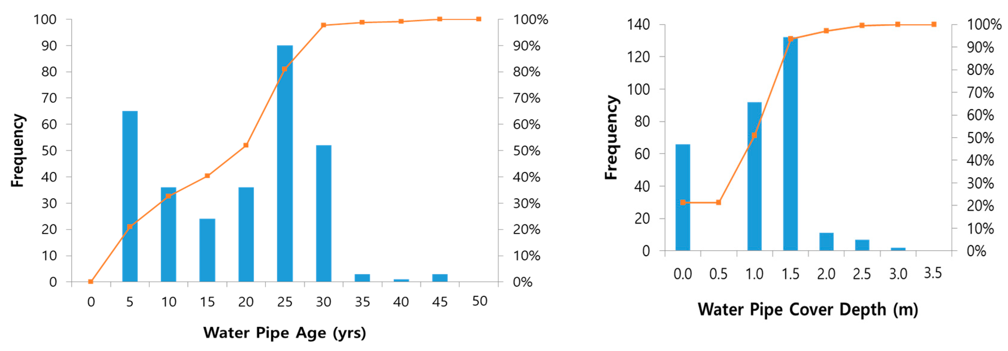
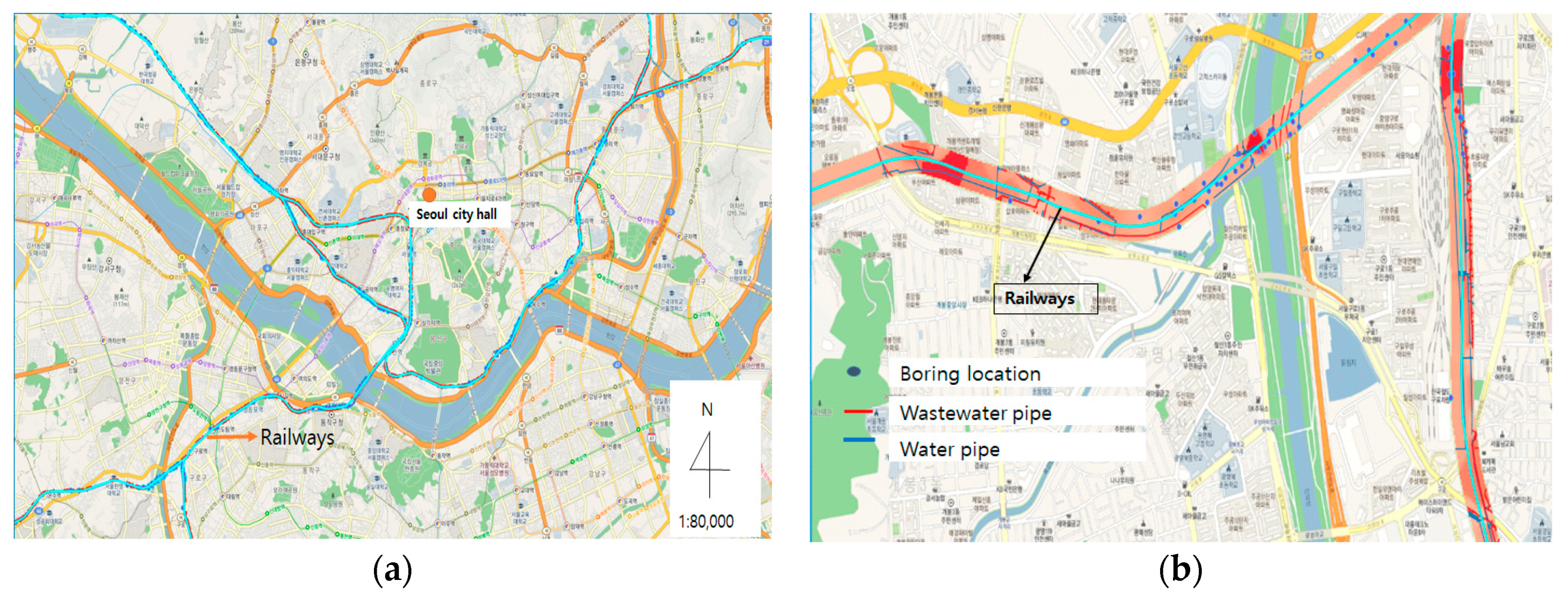
2. Establishing of Database

In order to establish the risk model, extensive efforts were made to integrate a water and sewer pipe databases to where the ground subsidences have taken place. Oh et al. [12] conducted a series of numerical analyses to examine the impact of ground subsidence on the railroad, as presented in Figure 2. The Mohr–Coulomb plasticity theory was applied for the plain strain 15-node element, and the ground condition was assumed to be weathered soil and rock, properties that account for the majority of the railroad roadbed in South Korea. With respect to the loading condition, 50 kPa of static distributed load was applied along the upper subgrade layer.

Parametric numerical analysis yielded a critical depth of underground cavities, with sizes of 1.5 m and 3.0 m, respectively, taking into account realistic design practice [13]. The position of underground cavities varied from one to five locations, as illustrated in Figure 2, and the vertical displacement of the upper subgrade was predicted.

It was found that when the underground cavity was located in the No. 3 position, as in Figure 2, the displacement of the railroad tended to drastically decrease. Based on this finding, a lateral spacing of 25 m with respect to the center of the railroad was considered as the influential zone, and thus the corresponding data was extracted within this zone.

The following data was mainly summarized and analyzed: pipe age in years, pipe cover depth in meters, pipe diameter in meters, and pipe length in meters. Figure 3 shows the distribution of water pipe data obtained in the location where the ground subsidences occurred. As noted, while the number of relatively new pipes (less than 10 years) is increasing due to the increase of residents and business sectors within this area, the amount of old pipes (more than 25 years) is also magnificent. In terms of the cover depth, most of the water pipes are buried within 1.5 m. Although the range of depth coverage seems to be suitable in accordance with the regulation of underground utility installation, inadequate structural conditions due to improper backfilling and degradation of pipe material may result in the excessive ground subsidence.

Given the location information, the network of water and sewer pipe systems along the railroad was embedded in the mapping system.

3. Risk Model

In this subsection, the support vector machine (SVM) [10] and multi-layer perceptron (MLP) [11] methods were employed to develop a risk model. They have been used in a variety of pattern classification, data mining, and data analysis applications. To develop the risk model, two sets of databases were used: one represents the water and wastewater pipes dataset where the ground subsidences have taken place and the other collected data from the places without the event.

3.1. Support Vector Machine (SVM)

Support vector machine creates a hyperplane using the supervised learning method of input data and determines the class of data through hyperplane. Suppose that m data $X=\left\{X_1,X_2,\dots ,X_m\right\}$ for the water supply in a certain area are given, each of which is labeled with a binary class $Y_i\in \left\{-1,1\right\}$. If the ground subsidence occurs at the output of the SVM, $Y_i=1$ otherwise $Y_i=-1$. The goal of the SVM is to design a decision hyperplane $Y_i=W^T{x}_i+w_0\mathrm{for}i=1,\dots ,m$ which maximally separates two classes, $S_{+}=\left\{x_j|Y_j=1\right\}$ and $S_{-}=\left\{x_j|Y_j=-1\right\}$ where $W$ and $w_0$ are the weight and bias of the decision function, respectively as shown in Figure 4. In other words, SVMs are trained with samples from two classes for finding the maximum-margin (shaded area in Figure 4) hyperplane. Samples on the margin are called the support vectors. Further, the general SVM model can predict which class the data belongs to; however, unlike the logistic regression model, the probability of belonging to each class cannot be calculated. To overcome this problem, a probabilistic SVM [14] model was used to estimate posterior probability using the distance between the test data and the hyperplane.

3.2. Multi-Layer Perceptron (MLP)

Multi-layer perceptron imitates the human brain to perform intelligent tasks [15]. It can represent complicated relationships between input and output and acquire knowledge about these relationships directly from the data. Suppose we are given a data set $X=\left\{X_1,X_2,\dots ,X_m\right\}$ for the water supply in a certain area, and each $X_n=[x_1^n,x_2^n,\dots ,x_d^n]{}^T(n=1,2,\dots ,m)$ belongs to one of two classes (the ground subsidence occurs or vice versa). The output of the MLP, as shown in Figure 5, is represented by

$$g_l(X_n)=f({\displaystyle \sum _{j=1}^{n_h}{w}_{lj}^{oh}}f({\displaystyle \sum _{i=1}^d{w}_{ji}^{hi}{x}_i^n+w_{j0})+w_{l0})(l=1,2)}$$

(1)

where $w_{ji}^{hi}$ is a weight between the ith input node and the jth hidden node, $w_{lj}^{oh}$ is a weight between the jth hidden node and the lth output node, $n_h$ is the number of hidden nodes, and $f(\cdot )$ is a actuation function.

We train the neural network such that the output $g_l(X_n)$ approaches the target value

$$\begin{array}{l}t(X_n)=[t_1,t_2,\dots ,t_C]{}^T,\\ t_l(X_n)=\{\begin{array}{cc}1\hfill & if{X}_n\in {\omega }_{\mathrm{l}}\hfill \\ 0\hfill & otherwise\hfill \end{array}(l=1,2,\dots ,C).\end{array}$$

(2)

As in [16], the network parameters are chosen to minimize the following function

$$\begin{array}{cc}J(W)& ={\displaystyle \sum _{n=1}^N{\displaystyle \sum _{l=1}^C{[g_l(X_n)-t_l(X_n)]}^2}}\hfill \\ & ={\displaystyle \sum _{l=1}^C({\displaystyle \sum _{X_n\in {\omega }_l}{[g_l(X_n)-1]}^2+}{\displaystyle \sum _{X_n\notin {\omega }_l}{[g_l(X_n)-0]}^2})}\hfill \\ & =N{\displaystyle \sum _{l=1}^C\left\{\frac{N_l}{N}\frac{1}{N_l}{\displaystyle \sum _{X_n\in {\omega }_l}{[g_l(X_n)-1]}^2+}\frac{N-N_l}{N}\frac{1}{N-N_l}{\displaystyle \sum _{X_n\notin {\omega }_l}{[g_l(X_n)-0]}^2}\right\}}\hfill \end{array}$$

(3)

Here, $W$ is the weight vector of the network, and $N_l$ is the number of samples belong to ${\omega }_l$. In the limit of infinite data, we can use Bayes’ formula to express (3) as

$$\begin{array}{c}\underset{N\to \infty }{\lim }\frac{1}{N}J(W)\equiv \tilde{J}(W)\hfill \\ ={\displaystyle \sum _{l=1}^C\left\{P({\omega }_l){\displaystyle \int {(g_l(X_n)-1)}^{2}p(X_n|}{\omega }_l)d{X}_n+P({\omega }_{i\ne l}){\displaystyle \int g_l{(X_n)}^{2}p(X_n|}{\omega }_{i\ne l})d{X}_n\right\}}\hfill \\ ={\displaystyle \sum _{l=1}^C\left\{{\displaystyle \int g_l{(X_n)}^{2}p(X_n)}d{X}_n-2{\displaystyle \int g_l(X_n)p(X_n,{\omega }_l)}d{X}_n+{\displaystyle \int p(X_n,{\omega }_l)}d{X}_n\right\}}\hfill \\ ={\displaystyle \sum _{l=1}^C\left\{{\displaystyle \int {[g_l(X_n)-P({\omega }_l|X_n)]}^{2}p(X_n)}d{X}_n+{\displaystyle \int P({\omega }_l|X_n)P({\omega }_{i\ne l}|X_n)p(X_n)}d{X}_n\right\}}\hfill \end{array}$$

(4)

Since the second term in Equation (4) is independent of $W$, to minimize $\tilde{J}(W)$, we obtain

$$g_l(X_n)\approx P({\omega }_l|X_n).$$

(5)

Therefore, we can compute the probabilities of ground subsidence occurrences by using output values of MLP [11].

3.3. Evaluation of Risk Model

The 310 water and 101 wastewater data were obtained within 50 m of the area where ground subsidences occurred. Furthermore, 154 water and 828 wastewater data were collected at the locations where the events had not occurred.

Table 1. Examples of data for computing the risk level.

Pipe Type	Installation Date	Diameter (m)	Length (m)	Average Depth (m)
Water	19 October 2011	1.00	14.62	1.10
Wastewater	1 January 1997	4.50	59.09	2.00
Wastewater	1 January 1989	7.00	4.01	5.00

shows the examples of water and wastewater data collected.

As shown in the Table 1, the main attributes of the water and wastewater data were installation date, diameter, length, and average cover depth. In this study, polynomial and radial basis function (RBF) kernel techniques were used for SVM approach in order to map the given data to the new vector space. The classification performance of the SVM with polynomial and the RBF kernel is shown in

Table 2. Analysis of water risk prediction model using Support Vector Machine (SVM).

Water Supply Risk Prediction	Indicator of Event	No. of Event		Classification Accuracy (%)	Overall Accuracy (%)
		0.00	1.00
Polynomial kernel	0.00	99	55	64.3	81.5
	1.00	31	279	90.0
Radial basis function (RBF) kernel	0.00	112	42	72.7	86.6
	1.00	20	290	93.5

.

In the table, indicator of event “0.00” represents the absence of ground subsidence and “1.00” the presence of it. The classification accuracy based on the polynomial kernel was 81.5% and the accuracy based on the RBF kernel was 86.6%. Overall, the prediction accuracy for the presence of event was superior to that of the absence of event case. As stated earlier, MLP creates a hidden layer between input and output layers to learn the weights and bias of nodes belonging to the three layers. The classification accuracy was measured by varying the number of hidden nodes which are the neurons in the hidden layer to establish a water supply risk model.

As presented in

Table 3. Analysis of water risk prediction model using Multi-Layer Perceptron.

Water Supply Risk Prediction	Indicator of Event	No. of Event		Classification Accuracy (%)	Overall Accuracy (%)
		0.00	1.00
Hidden node: 100	0.00	126	28	81.8	89.9
	1.00	19	291	93.9
Hidden node: 300	0.00	132	22	85.7	92.2
	1.00	14	296	95.5
Hidden node: 500	0.00	127	27	82.5	90.3
	1.00	18	292	94.2
Hidden node: 700	0.00	135	19	87.7	92.7
	1.00	15	295	95.2

, the classification accuracy of absence of the event case (87.7% with the number of hidden nodes of 700) was significantly improved compared to the SVM model. As the number of hidden nodes increased, higher accuracy was generally achieved. The wastewater risk model was also assembled using the SVM and MLP. Similar to water risk model assessment, RBF and polynomial functions were used as SVM kernel functions, and their performance is shown in

Table 4. Analysis of wastewater risk prediction model using SVM.

Wastewater Supply Risk Prediction	Indicator of Event	No. of Event		Classification Accuracy (%)	Overall Accuracy (%)
		0.00	1.00
Polynomial kernel	0.00	827	1	99.9	89.6
	1.00	96	5	5.0
RBF kernel	0.00	818	10	98.8	90.3
	1.00	80	21	20.1

.

In Table 4, the overall classification accuracy is as high as 89.6% and 90.3%; however, it should be noted that the classification accuracy of the presence of the event was substantially low compared to the water risk model. This is attributed to the fact that wastewater risk model was trained with a relatively imbalanced dataset between the absence and presence of ground subsidence cases, unlike the water risk datasets.

Table 5. Analysis of wastewater risk prediction model using MLP.

Wastewater Supply Risk Prediction	Indicator of Event	No. of Event		Classification Accuracy (%)	Overall Accuracy (%)
		0.00	1.00
Hidden node: 100	0.00	799	29	96.5	89.3
	1.00	37	64	36.6
Hidden node: 300	0.00	810	18	97.8	91.6
	1.00	60	41	40.6
Hidden node: 500	0.00	809	19	97.7	92.8
	1.00	48	53	52.5
Hidden node: 700	0.00	807	21	97.5	93.3
	1.00	41	60	59.4

presents the results of the wastewater risk model assessment using the MLP model. The classification accuracy of the presence of the event case was improved compared to that of the SVM model. Consequently, the MLP model was chosen for the risk model of water supply and wastewater utilities due to the enhancement in terms of classification accuracy in case of presence of the event.

Further, to utilize the risk model, a simple program was developed in the Matlab environment to compute the probability of risk.

4. Field Evaluation of Risk Model

Incorporating the risk model established herein, this study developed a QGIS-based mapping system as illustrated in Figure 6. Figure 6a shows the railway networks of the Seoul area in the hazard map system and Figure 6b shows the variation of risk levels of tested locations boxed in Figure 6a. This system enables users to view the distribution of risk level along with inventory data that includes basic geotechnical boring data, water supply and wastewater utility’s age, cover depth, length, etc., if available. The geological risk model was developed based on regression analysis taking into account the ground water level, alluvial layer thickness, and standard penetration test (SPT) data as follows.

$$\mathrm{Geological}\mathrm{risk}=\frac{\exp \left(-0.441\times G.T-0.505\times T+0.183\times SP{T}_N+4.471\right)}{1+\exp \left(-0.441\times G.T-0.505\times T+0.183\times SP{T}_N+4.471\right)}$$

(6)

Where, GT is the groundwater table in meters, T is the alluvial layer thickness in meters, and SPT_N is the sum of the number of blows required for the second and third 150 mm of penetration from SPT test. The total risk index can be calculated using Equation (7), and is classified into five categories as shown in

Table 6. Description of risk index in the hazard map system.

Total Risk Index (%)	Description
80~100	Very high risk requires closing the line for repair
65~79	High risk requires immediate maintenance action
50~64	Medium risk requires periodic maintenance action
25~49	Low risk requires a maintenance plan
<25	Very low risk requires no maintenance action

.

Total risk index (%) = (Geological risk) × 0.2 + (Water pipe risk) × 0.4 + (Wastewater pipe risk) × 0.4

(7)

Figure 7 illustrates the procedure to quantify the risk level in the hazard map system.

In this study, field validation of the established risk model was conducted using a nondestructive survey and pneumatic cone penetration (PCP) test. Twelve field test sections were selected based on the risk index represented from low to high. A series of nondestructive surveys were then conducted using a 500 MHz antenna equipped with ground penetrating radar (GPR) and electrical resistance (ER) survey installing twelve electrodes with one-meter spacing to investigate the following: the presence of buried utilities, abnormality of ground condition, and the presence of underground cavities. Once the nondestructive test was completed, PCP tests were conducted at the locations where abnormalities of ground were detected and normal locations for comparison. Figure 8 shows examples of nondestructive test results.

As shown in Figure 8, as risk indices increase, the subsurface profile obtained from GPR becomes irregular, and the average ER values become relatively lower. To determine the average ER values per test section, image analysis was employed to quantify the area of individual ER zones. Once the area was quantified for individual ER zones, the weighted average considering the quantified area was then computed to represent the test section. In this manner, the ER survey was found to be effective in the assessment of risk index along with GPR survey, which was useful to detect the presence of buried utilities as long as the depth of cover was within 3 m. Pneumatic cone penetration testing was conducted in accordance with DIN ISO 22476-2 up to 2 m below the surface. The PCP tests had an advantage of penetrating deeper depths with constant impact energy, controlled by pneumatic force, compared to a typical dynamic cone penetrometer test. From this test, two indices were assigned to evaluate the bearing capacity of subsurface. For instance, N₅₀ indicates the number of blows to penetrate the pneumatic cone up to 0.5 m. Higher numbers of blows indicates larger load bearing capacity of the subsurface. Generally, the number of blows tends to decrease at the locations where abnormality of ground was detected compared to normal conditions. The relationships between average electrical resistivity, the number of blows from PCP tests, and the risk index were established based on the risk model, as shown in Figure 9. The N-value of PCP test was found to have a promising relationship with risk index and average electrical resistivity even though the R-square value was not sufficiently high to ensure statistical accuracy. Consequently, it was deemed that further research needed to be conducted to validate this relationship.

5. Concluding Remarks

Damage from aged underground utilities in metropolitan areas was found to be the primary cause of ground subsidence in this study. The present paper developed a risk model to assess the probability of ground subsidence along railways surrounding the Seoul area of the Republic of Korea. The following conclusions and perspectives can be obtained.

(1)

Between the two approaches (i.e., SVM and MLP) employed in this study to develop a risk model, the MLP approach was found to be more efficient by improving the classification accuracy of the presence of ground subsidence.

(2)

The number of hidden nodes played a significant role in determining overall accuracy of the risk model. Considering the number of input data for water and wastewater pipes (564 for water and 929 for wastewater pipes), it was deemed appropriate to have more hidden nodes than inputs to ensure the reliability of the risk model. A previous study recommended that the number of hidden nodes be 1.5 times the number of parameters in the input layer [17].

(3)

A series of field experimental programs using GPR, ER survey, and PCP tests exhibited that the correlations between measurements seemed to be promising in the assessment of the risk index with respect to ground subsidence in spite of limited field validations. It is strongly recommended that further investigation needs to be done to verify this finding in the near future. Ground penetrating radar survey is useful to visually detect underground utilities and underground homogeneity. Electrical resistance survey gives the variation of electrical resistance, which can be quantified for the tested section. Pneumatic cone penetration testing provides bearing capacity of tested ground, which is associated with risk index and ER values. Consequently, the use of hazard map systems in conjunction with field investigation is recommended as a proactive approach to mitigate the progress of ground subsidence along railways.

References

1. Seoul Metropolitan Government. Investigation of Underground Cavity Mechanism; Research Report; Seoul Metropolitan Government: Seoul, Korea, 2015.
2. Al-Kouri, O.; Al-Fugara, A.; Al-Rawashdeh, S.; Sadoun, B.; Pradhan, B. Geospatial Modeling for Sinkholes Hazard Map based on GIS&RS Data. J. Geog. Inf. Syst. 2013, 5, 584–592. [Google Scholar]
3. Klimchouk, A. Morphogenesis of hypogenic caves. Geomorphol. 2009, 106, 100–117. [Google Scholar] [CrossRef]
4. USGS. Available online: https://www.usgs.gov/faqs/what-difference-between-a-sinkhole-and-land-subsidence?qt-news_science_products=0#qt-news_science_products (accessed on 20 September 2018).
5. Galve, J.P.; Remondo, J.; Gutierrez, F. Improving sinkhole hazard models incorporating magnitude–frequency relationships and nearest neighbor analysis. Geomorphol. 2011, 134, 157–170. [Google Scholar] [CrossRef]
6. Galve, J.P.; Gutierrez, F.; Lucha, P.; Bonachea, J.; Remondo, J.; Cendrero, A.; Gutierrez, M.; Gimeno, M.J.; Pardo, G.; Sanchez, J.A. Sinkholes in the Salt-bearing evaporate karst of the Ebro River valley upstream of Zaragoza city (NE Spain) Geomorphological mapping and analysis as a basis for risk management. Geomorphology 2009, 108, 145–158. [Google Scholar] [CrossRef]
7. Zhao, A.; Tang, A. Land subsidence risk assessment and protection in mined-out regions. Proc. IAHS 2015, 372, 145–150. [Google Scholar] [CrossRef] [Green Version]
8. Park, J.K.; Cho, D.H.; Hossain, M.S.; Oh, J. Assessment of Settlement Profile Caused by Underground Box Structure Installation with an Artificial Neural Network Model. J. Transp. Res. Board 2018. [Google Scholar] [CrossRef]
9. Park, H.I. Study for Application of Artificial Neural Networks in Geotechnical Problems. In Artificial Neural Networks-Application; IntechOpen: Rijeka, Croatia, 2011. [Google Scholar] [Green Version]
10. Lee, H.; Kim, E. Genetic outlier detection for a robust support vector machine. Int. J. Fuzzy Log. Intell. Syst. 2015, 15, 96–101. [Google Scholar] [CrossRef]
11. Lee, H.; Hong, S.; Kim, E. A new genetic feature selection with neural network ensemble. Int. J. Comput. Math. 2009, 1105–1117. [Google Scholar]
12. Oh, J.; Kim, J.; Choi, J.; Kim, K. Smart Evaluation of Railroad Roadbed with Respect to the Ground Subsidence; Final Research Report No. 2017-50102-002; Korea Rail Network Authority: Daejeon, Korea, 2016. [Google Scholar]
13. Yoo, H.; Oh, J. Mechanical and chemical reinforcements for the installation of underground utilities to mitigate underground cavity. J. Korean Soc. Hazard Mitig. 2017, 17, 257–268. [Google Scholar] [CrossRef]
14. Oh, K.; Lee, H.; Hong, S.; Kim, E. Side view face recognition as an aid to gait recognition. In Proceedings of the Joint 3rd International Conference on Soft Computing and Intelligent Systems and 7th International Symposium on Advanced Intelligent Systems, Japan Society for Fuzzy Theory and Intelligent Informatics, Tokyo, Japan, 20–24 September 2006; pp. 490–495. [Google Scholar]
15. Hagan, M.T.; Demuth, H.B.; Beale, H. Neural Network Design; PWS Publishing Company: Boston, MA, USA, 1995. [Google Scholar]
16. Suen, C.Y.; Nadal, C.; Mai, T.; Legaulr, R.; Lam, L. Recognition of handwritten numerals based on the concept of multiple experts, In Proceedings of the 1st International Workshop on Frontiers Handwriting Recognition: Montreal, QC, Canada, 2–3 April 1990; pp. 131–144. [Google Scholar]
17. Mamaqani, B. Numerical Modeling of Ground Movements Associated with Trenchless Box Jacking Technique. Ph.D. Thesis, The University of Texas, Arlington, TX, USA, 2014. [Google Scholar]
Figure 1. (a) A snapshot of ground subsidence in Seoul and (b) number of ground subsidence that occurred in Seoul between 2010 and 2014.
Applsci 08 01936 g001
Figure 2. (a) Numerical analyses of geometric conditions and material properties conducted and (b) Parametric evaluations on the potions of underground cavity [12].
Applsci 08 01936 g002
Figure 3. Distribution of water pipe age and cover depth.
Applsci 08 01936 g003
Figure 4. Support vector machine (SVM) model.
Applsci 08 01936 g004
Figure 5. Multi-layer perceptron (MLP) model.
Applsci 08 01936 g005
Figure 6. (a) Railways of Seoul in mapping system and (b) a close-up example of tested locations showing different risk levels.
Applsci 08 01936 g006
Figure 7. Procedure to determine the risk index in the hazard map system.
Applsci 08 01936 g007
Figure 8. Examples of nondestructive test results.
Applsci 08 01936 g008
Figure 9. Relationship between field measurements; (a) N-value versus average electrical resistivity and (b) N-value versus risk index.
Applsci 08 01936 g009