A Fast Three-Dimensional Display Method for Time-Frequency Spectrogram Used in Embedded Fault Diagnosis Devices

Abstract

Time-frequency analysis is usually used to reveal the appearance of different frequency components varying with time, in signals, of which time-frequency spectrogram is an important visual tool to display the information. The Mesh Surface Generation (MSG) algorithm is widely used in three-dimensional (3D) modeling. Removing hidden lines from the mesh plot is an essential process that produces explicit depth information. In this paper, a fast and effective method has been proposed for a time-frequency Spectrogram Mesh Surface Generation (SMSG) display, especially, based on the painter’s algorithm. In addition, most portable fault diagnosis devices have little function to generate a 3D spectrogram, which generally needs a general computer to realize the complex time-frequency analysis algorithms and a 3D display. However, general computer is not portable and then not suitable for field test. Hence, the proposed SMSG algorithm is applied to an embedded fault diagnosis device, which is light, low-cost, and real-time. The experimental results show that this approach can realize a high degree of accuracy and save considerable time.

1. Introduction

Time-frequency analysis is an effective method to detect machine faults under variable speed conditions [1]. The conventional time-domain or frequency-domain analysis cannot fully describe the real-life signal, whose frequency content varies with time [2]. 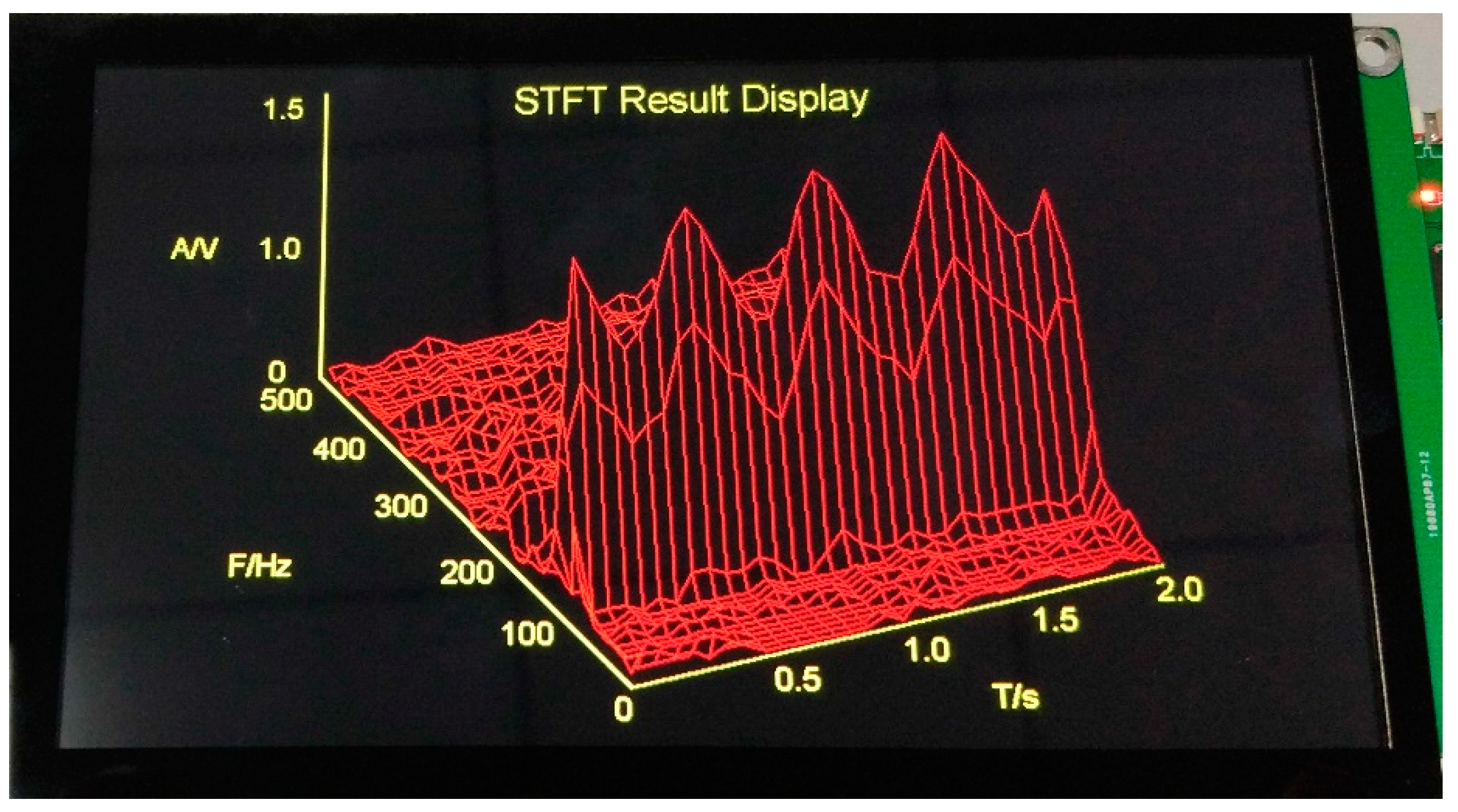To gain frequency-related, as well as time-related information, of non-stationary and non-periodic signals, it is recommendable to use analysis in time-frequency domain [3]. In the process of fault diagnosis and condition monitoring, it is often necessary to display 3D graphics under different working conditions [4]. For example, the Short-Time Fourier transform (STFT) of signals require a time-frequency distribution map, for precise analyzing.

The most common tool used for fault diagnosis and 3D display is general purpose computers, such as Personal Computers (PC) [5]. Usually the signal data will be collected in fields and then be taken to a PC for a thorough analysis. For example, a computer-based method for rolling element bearing defect diagnosis, under a variable speed operation, through an angel synchronous averaging of wavelet denoising estimation has been suggested in previous articles [6]. This kind of an online method can be powerful and comprehensive but also suffers from some drawbacks, such as not being a real-time system, having a long period, being expensive, and not being portable to transport [7].

Embedded fault diagnosis devices are widely used in field testing, due to their good performance, in terms of size, and ease of showing wave forms on a Liquid Crystal Display (LCD) screen, in real time. However, at present, most of the embedded fault diagnosis devices can only provide two-dimensional (2D) forms, such as time-domain waves or frequency spectrum waves. Among them, Guven and Atis have analyzed rotor bar failures, based on the obtained Fast Fourier Transform spectrum in embedded systems [8]. Lu et al. have successfully displayed several envelope-order spectrums of motor bearing vibration signals in a portable device [9]. In this paper, an embedded system, instead of a traditional PC, is used to carry out the time-frequency analysis and the three-dimensional (3D) time-frequency spectrogram display.

MSG is a very common method in finite element modeling. The idea of using a mesh surface to represent 3D graphics is referenced and is specially applied to a spectrogram display, in this paper. In order to get correct 3D graphics, a very important problem—Hidden Surface Removal (HSR) must be solved. The commonly used algorithms of HSR, include the painter’s algorithm, the Z-buffer algorithm, and the BSP tree algorithm [10]. Among these classical methods, the painter’s algorithm is the most suitable way for dealing with the HSR problem of simple polygons. For example, Richard et al. have implemented a painter’s algorithm to render poly-ranges in a multiple-view oceanographic visualization system [11]. A kind of space hidden method of 2.5D statistical cartographic symbols, based on the painter’s algorithm was put forward in a study by Zhang et al. [12]. Li et al. has established the occlusion model of truck, by applying the painter’s algorithm [13]. However, there are few methods for 3D display in embedded devices. The painter’s algorithm suffers from high complexity, heavy system spending, and long computation time. It cannot be used directly in embedded devices, which have limited memory sizes and strict timeliness requirements [8].

In this paper, a Spectrogram Mesh Surface Generation (SMSG) algorithm for a time-frequency spectrogram display is presented, and the method is applied to an embedded fault diagnosis system. Although the method is based on the painter’s algorithm, it requires no sorting algorithm for time-frequency spectrograms. Therefore, it costs little time and the graph can be rotated with a certain angle for observation, during the drawing process. The proposed algorithm can also be applied to plot other parametric equation surfaces.

2. Materials and Methods

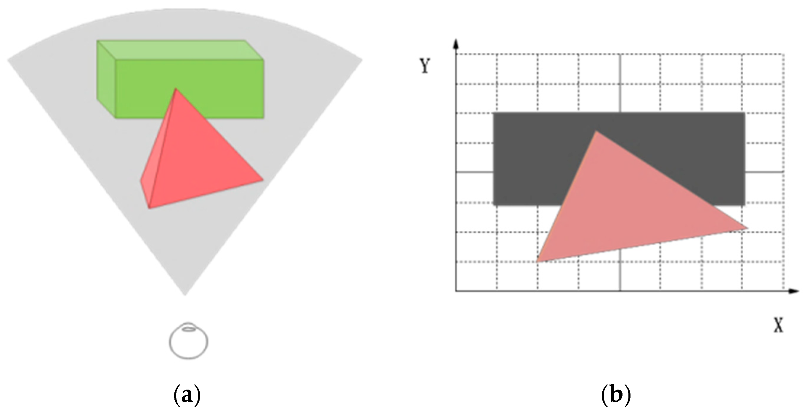
The principle of the SMSG algorithm is mainly based on the painter’s algorithm, also known as depth-sorting algorithm [14]. It is the same as when observing two objects, the frontal object obscures the back one. For example, there is a cuboid and a tetrahedron in Figure 1a, the cube being behind the tetrahedron. It can be seen from Figure 1b that the overlapped part of the two objects, especially a part of the cube is covered and is not visible. When drawing the graph, the HSR displaying was realized [15].

There are two commonly used projection methods—orthogonal projection and perspective projection. An orthogonal projection means that no matter how far away from the view point (eyes or a camera), the size of the projected object remains unchanged. Unlike 3D models, such as convex polyhedron and concave polyhedron, there is no need to produce a significant perspective effect in time-frequency spectrogram. Additionally, the computational cost of orthogonal projection is less than that of perspective projection. Therefore, the orthogonal projection has been used for generating 3D figures, in this paper.

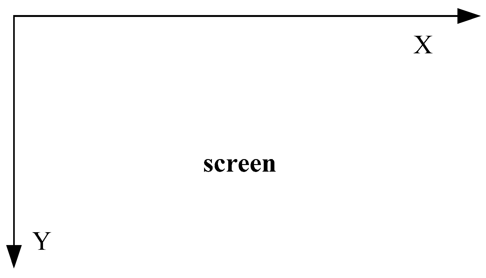
To draw 3D graphics on a computer, or an embedded device, more specifically, means to draw the projection figure of 3D objects on a certain plane, at a certain angle. The screen coordinates used in the LCD is shown in Figure 2, where the Z-axis is perpendicular to the LCD screen. Here, the XOY-plane was chosen as the projection plane. The viewpoint was located at the positive infinity of the Z-axis.

The formula of the orthogonal projection is shown in Equation (1):

$$\left[\begin{array}{cccc}{x}^{\prime }& y^{\prime }& z^{\prime }& 1\end{array}\right]=\left[\begin{array}{cccc}x& y& z& 1\end{array}\right]·\left[\begin{array}{cccc}1& 0& 0& 0\\ 0& 1& 0& 0\\ 0& 0& 0& 0\\ 0& 0& 0& 1\end{array}\right]$$

(1)

[x, y, z] was the homogeneous coordinate of a point in 3D space, and [x^′, y^′, z^′] was the orthogonal projection coordinate. According to Equation (1), the Z-axis value was omitted if orthogonal projection was performed directly. To produce a three-dimensional effect, it was necessary to rotate the coordinates around the X-axis and the Y-axis, by a certain angle.

When a degree of α was rotated around the X-axis, the transformation formula was as follows:

$$\left[\begin{array}{cccc}{x}^{\prime }& y^{\prime }& z^{\prime }& 1\end{array}\right]=\left[\begin{array}{cccc}x& y& z& 1\end{array}\right]·\left[\begin{array}{cccc}1& 0& 0& 0\\ 0& \cos \alpha & \sin \alpha & 0\\ 0& -\sin \alpha & \cos \alpha & 0\\ 0& 0& 0& 1\end{array}\right]$$

(2)

When a degree of β was rotated around the Y-axis, the transformation formula was as follows:

$$\left[\begin{array}{cccc}{x}^{\prime }& y^{\prime }& z^{\prime }& 1\end{array}\right]=\left[\begin{array}{cccc}x& y& z& 1\end{array}\right]·\left[\begin{array}{cccc}\cos \beta & 0& -\sin \beta & 0\\ 0& 1& 0& 0\\ \sin \beta & 0& \cos \beta & 0\\ 0& 0& 0& 1\end{array}\right]$$

(3)

It is important to note that α and β were positive rotation angles in the right-handed coordinate system.

Given a point (x, y, z) in the three dimensions, when rotating α degree around the X-axis, the coordinate changed to:

$$\{\begin{array}{c}x\prime =x\\ y\prime =y\cos \alpha -z\sin \alpha \\ z\prime =y\sin \alpha +z\cos \alpha \end{array}$$

(4)

If a degree of β was rotated around the Y-axis, then Equation (5) could be updated with Equation (4), from which Equation (6) could be obtained:

$$\{\begin{array}{c}x\prime =z\sin \beta +x\cos \beta \\ y\prime =y\\ z\prime =y\cos \beta -x\sin \beta \end{array}$$

(5)

$$\{\begin{array}{c}x\prime =(y\sin \alpha +z\cos \alpha )\sin \beta +x\cos \beta \\ y\prime =y\cos \alpha -z\sin \alpha \\ z\prime =(y\sin \alpha +z\cos \alpha )\cos \beta -x\sin \beta \end{array}$$

(6)

Finally, the orthogonal projection coordinate (x, y) was as follows:

$$\{\begin{array}{c}x\prime =(y\sin \alpha +z\cos \alpha )\sin \beta +x\cos \beta \\ y\prime =y\cos \alpha -z\sin \alpha \end{array}$$

(7)

The rotation order could be changed, which depended on the users’ need. The above formulas were only an example of rotation. As is shown in Equation (7), the depth value information of the Z-axis was contained in the orthogonal projection coordinate, after rotating by α and β degrees.

In some occasions, it might also be needed to rotate around the Z-axis by a certain angle of γ. Then the transformation formula should have been changed as follows:

$$\left[\begin{array}{cccc}{x}^{\prime }& y^{\prime }& z^{\prime }& 1\end{array}\right]=\left[\begin{array}{cccc}x& y& z& 1\end{array}\right]·\left[\begin{array}{cccc}\cos \gamma & \sin \gamma & 0& 0\\ -\sin \gamma & \cos \gamma & 0& 0\\ 0& 0& 1& 0\\ 0& 0& 0& 1\end{array}\right]$$

(8)

In this paper, the STFT algorithm was used as the time-frequency analysis method in the embedded fault diagnosis devices. Given a signal x(τ) and a sliding window function w(τ), the STFT of the signal x was defined as follows [16]:

$$F_x^w\left(t,f\right)={\displaystyle \int x\left(\tau \right)}{w}_{t,f}\left(\tau -t\right)e^{-j2\pi f\tau }\mathrm{d}\tau$$

(9)

Spectrogram was the squared magnitude of the STFT, expressed as the following:

$$\begin{array}{l}{S}_s^w\left(t,f\right)={\left|F_x^w\left(t,f\right)\right|}^2\\ ={\left|{\displaystyle {\int }_{-\infty }^{+\infty }s\left(\tau \right)w\left(\tau -t\right)e^{-2\pi f\tau }\mathrm{d}\tau }\right|}^2\end{array}$$

(10)

As is shown in Equation (10), the time-frequency spectrogram contained three-dimensional information—time (T), frequency (F), and amplitude (A). The joint time-frequency distribution matrix was a 2D array. Supposed that the signal length was L, the window length was W, and the sliding step was s, then the window number n could be obtained by Equation (11).

$$n=\mathrm{int}\left(\frac{L-W}{s}\right)+1$$

(11)

The matrix size was 2m × n, where 2m represented for 2m-point fast Fourier transform (FFT). Due to the symmetry of a Fourier transform, only the first half m × n data of the joint time-frequency distribution matrix was taken to display. Mesh surface was composed of longitude and latitude lines, corresponding to the intersection of time line and frequency line. Then the value of (f, t, a) in the joint time-frequency distribution matrix was corresponded to the value of (x, y, z), in the orthogonal projection formula.

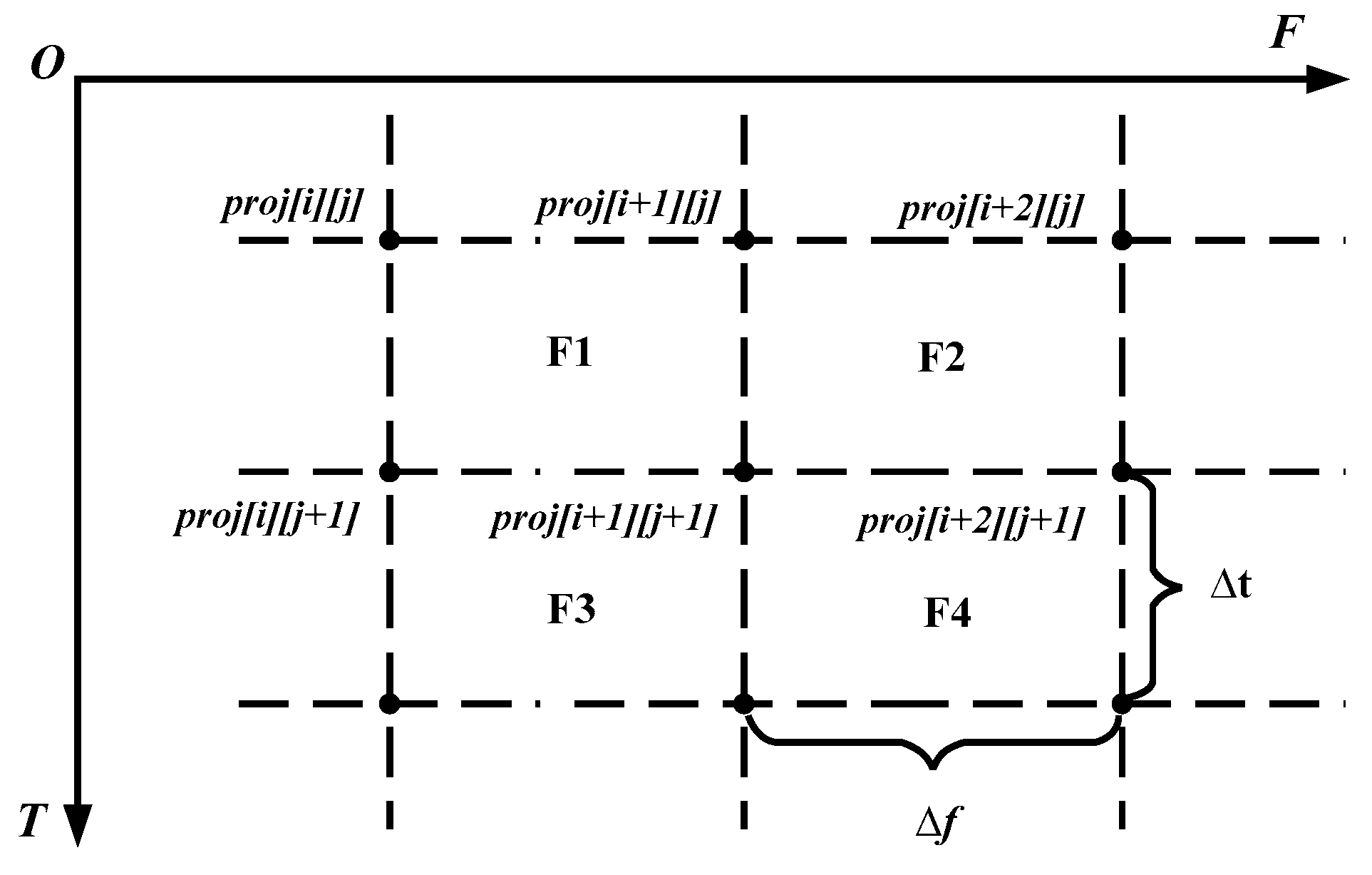
The proposed SMSG algorithm could be described by six steps.

Step 1: Frequency axis (X-axis) was divided into m equal units, and time axis (Y-axis) was divided into n equal units. Let ∆f and ∆t denote the length and width of the mesh unit, respectively. All the points in the joint time-frequency distribution matrix were formed into a 3D coordinate matrix p[m][n]. p[m][n] = (x_i, y_j, z_i,j) = (f_i, t_j, a_i,j).

Step 2: The coordinates of the points should be rotated by a certain angle around the X-axis, Y-axis, and Z-axis, based on actual demand.

Step 3: All 3D coordinates of p[m][n] was projected onto the 2D coordinates of proj[m][n], where proj[m][n] was obtained by an orthogonal projection of p[i][j].

Step 4: Starting with (i, j) = (0, 0), the four vertices of proj[i][j], proj[i + 1][j], proj[i + 1][j + 1] and proj[i][j + 1] were connected with a brush to form a mesh. Then the mesh surface was rendered with a different color.

Step 5: After each single mesh surface was drawn, the point of proj[i + 1][j] = (f_i + ∆f, t_j) would be dealt in a sequential order of frequency, namely along the positive direction of the X-axis. Then the next four vertices of proj[i + 1][j], proj[i + 2][j], proj[i + 2][j + 1], and proj[i + 1][j + 1] would be taken in turn. The process of this kind of filling mesh surfaces would be repeated, one by one.

Step 6: After each line of the mesh surfaces was drawn, the point of proj[0][j + 1] = (0, t_j + ∆t) would be dealt in the chronological order of time, that is, along the positive direction of the Y-axis. Additionally, the process of filling mesh surfaces would be repeated, line by line. As is shown in Figure 3, the mesh surface would be rendered as follows: F1 → F2 → … → F3 → F4.

When the algorithm was programmed in an embedded system, the above steps could be completed with two, for-loop nesting. Suppose i was updated once after each single surface was drawn: i = i + 1, and j was updated to: j = j + 1, after each line of mesh surfaces was drawn. The pseudo-code diagram is shown as follows (Algorithm 1).

Algorithm 1: SMSG Algorithm

INIT: thx ← α, thy ← β, thz ← γ;//rotation angle

f[m], t[n], a[m][n];//the STFT results

LOOP 1: obtain the 2D projection coordinates proj[m][n].

For i = 0; i < m; i = i + 1

For j = 0; j < n; j = j + 1

x ← f[i]; y ← t[j]; z ← a[i][j];

(x, y, z) ← (x, y, z) coordinates sequentially rotate thx, thy, thz;

proj[i][j].x ← orthogonal projection of x;

proj[i][j].y ← orthogonal projection of y;

proj[i][j].z ← orthogonal projection of z;

End For

End For

END LOOP 1

LOOP 2: generate the 3D mesh surface.

For j = 0; j < n − 1; j = j + 1

For i = 0; i < m − 1; i = i + 1

DrawPolygon(proj[i][j], proj[i + 1][j], proj[i + 1][j + 1], proj[i][j + 1]);

FillPolygon(proj[i][j], proj[i + 1][j], proj[i + 1][j + 1], proj[i][j + 1]);

End For

End For

END LOOP 2

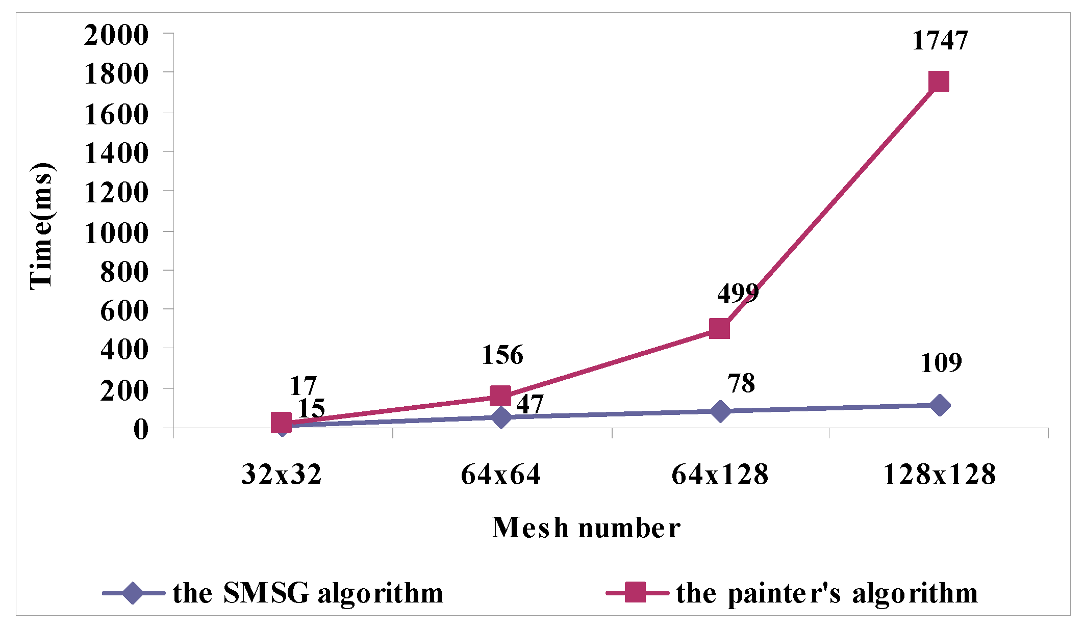
By defining M as the number of polygons in a scene, and N as the number of pixels in the resolution of the screen, it could be calculated that the SMSG algorithm had a complexity of O(MN). The efficiency of the painter’s algorithm essentially depends on the method of sorting which is a time consuming procedure. As in the worst case the complexity of a sorting algorithm, is O(N²), and the average complexity is O(NlogN) as shown in

Table 1. Time complexity of several common sorting algorithms.

Sorting Algorithm	The Best Case	The Worst Case	Average Case
Bubble sort	O(N2)	O(N2)	O(N2)
Insertion sort	O(N2)	O(N2)	O(N2)
Quicksort	O(NlogN)	O(N2)	O(NlogN)
Merge sort	O(NlogN)	O(NlogN)	O(NlogN)

[17], which gives the time complexity of several common sorting algorithms. It is important to note that the time complexity shown in Table 1 is only the complexity of sorting algorithms, not including the complexity of drawing operation of the painter’s algorithm, which also has the same complexity as that of the SMSG algorithm.

In addition, considering a user’s observation demand of the specific distribution of frequency values and its change trend with time, a Frequency-Time-Amplitude (F-T-A) coordinate system and a Time-Frequency-Amplitude (T-F-A) coordinate system would be needed to display. The default coordinate system of the above algorithm is the F-T-A coordinate system. If the user expects to observe the result in the T-F-A coordinate system, it only needs to perform an up-and-down flipping and a transpose operation of the joint time-frequency distribution matrix.

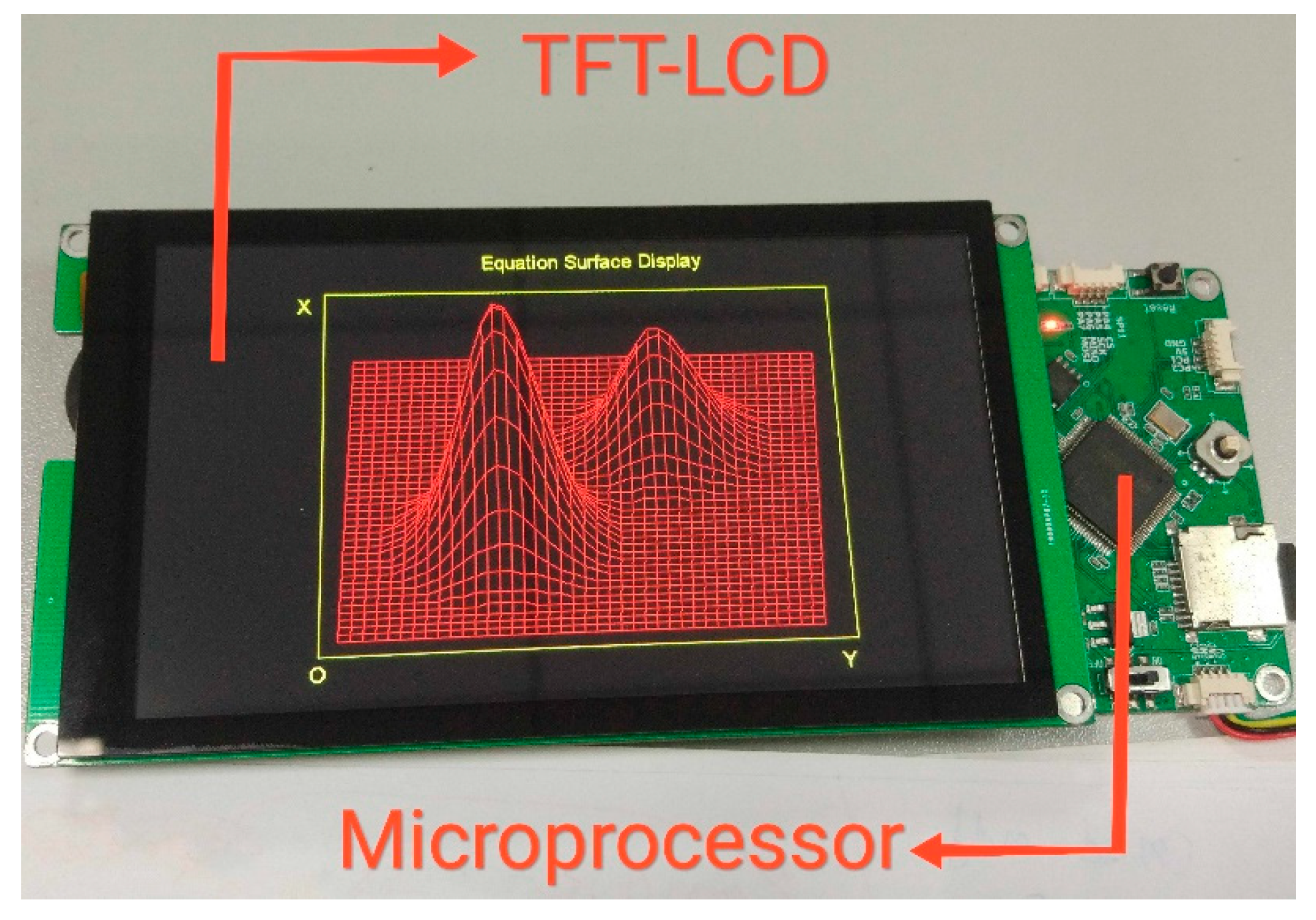
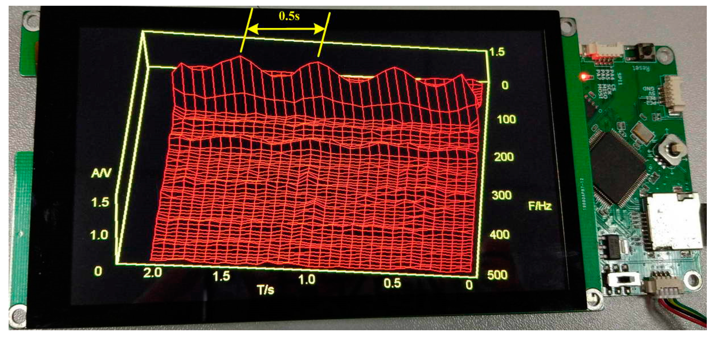
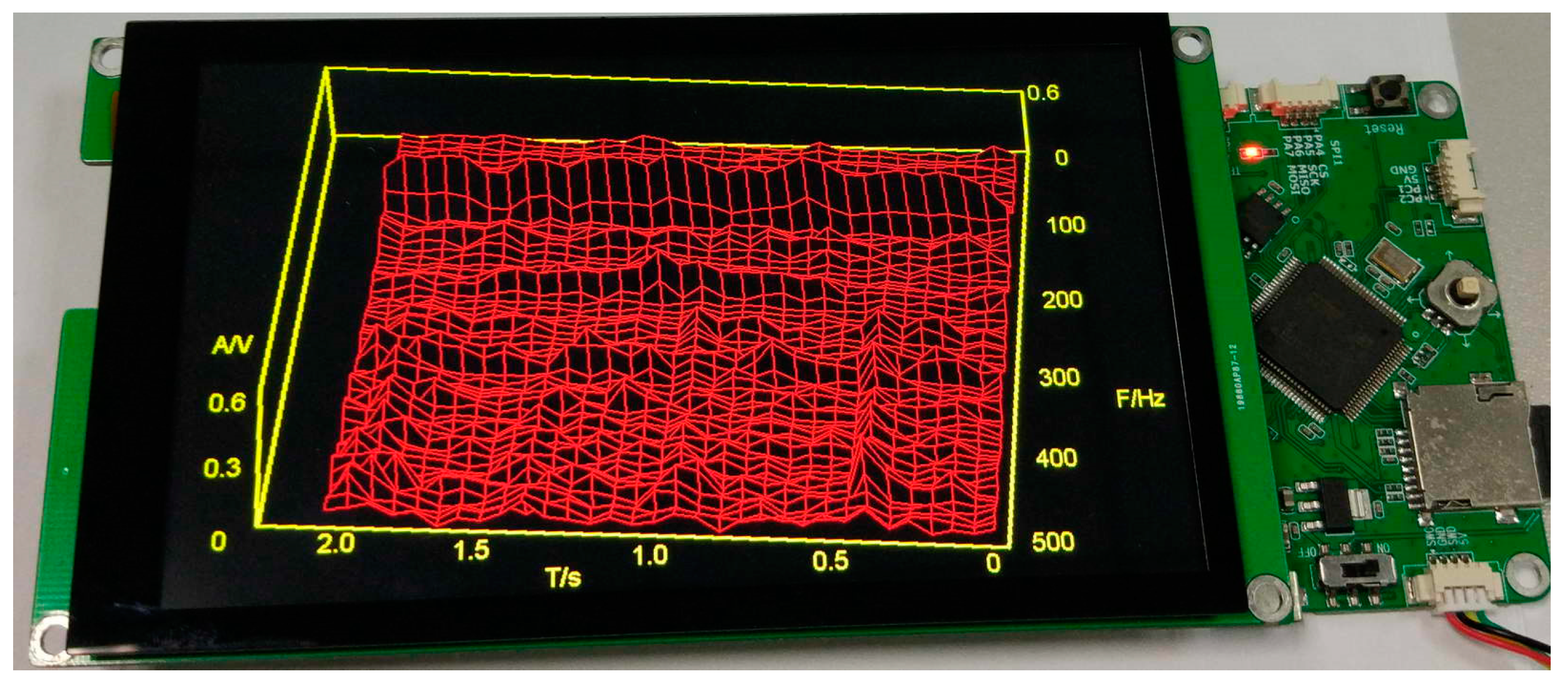
The embedded device used in this paper is shown in Figure 4. The hardware was composed of a STM32F407 microprocessor, a Thin Film Transistor LCD (TFT-LCD) module, a program download interface, and liquid crystal drive circuits. The operating frequency of the STM32F407 microprocessor was 168 MHz. The STM32F407 microprocessor was a 32-bit MCU, with float point units, and digital signal processor instructions, which was capable of handling complex calculation and analysis operations. The TFT-LCD supports up to 24 bit, 854 × 480 real color displays.

Firstly, the SMSG algorithm was implemented on a PC to validate its effectivity with the Visual C++ 6.0 software, which was developed by the Microsoft corporation in Redmond, Washington, U.S. in 1998. And then the results obtained by the MATLAB R2014a, which was designed by the MathWorks Company in Natick, Massachusetts, U.S. in 2014, were used to verify the correctness of the SMSG algorithm. Once the practicability was validated, the SMSG algorithm was realized in an embedded device with C language, which was usually used in the program of embedded systems. The comparison test was conducted on a computer with the following configurations: 2.6 GHz Inter Celeron CPU, 4.0 GB RAM, 64-bit WIN7 operation system, MATLAB R2014a, and Visual C++ 6.0.

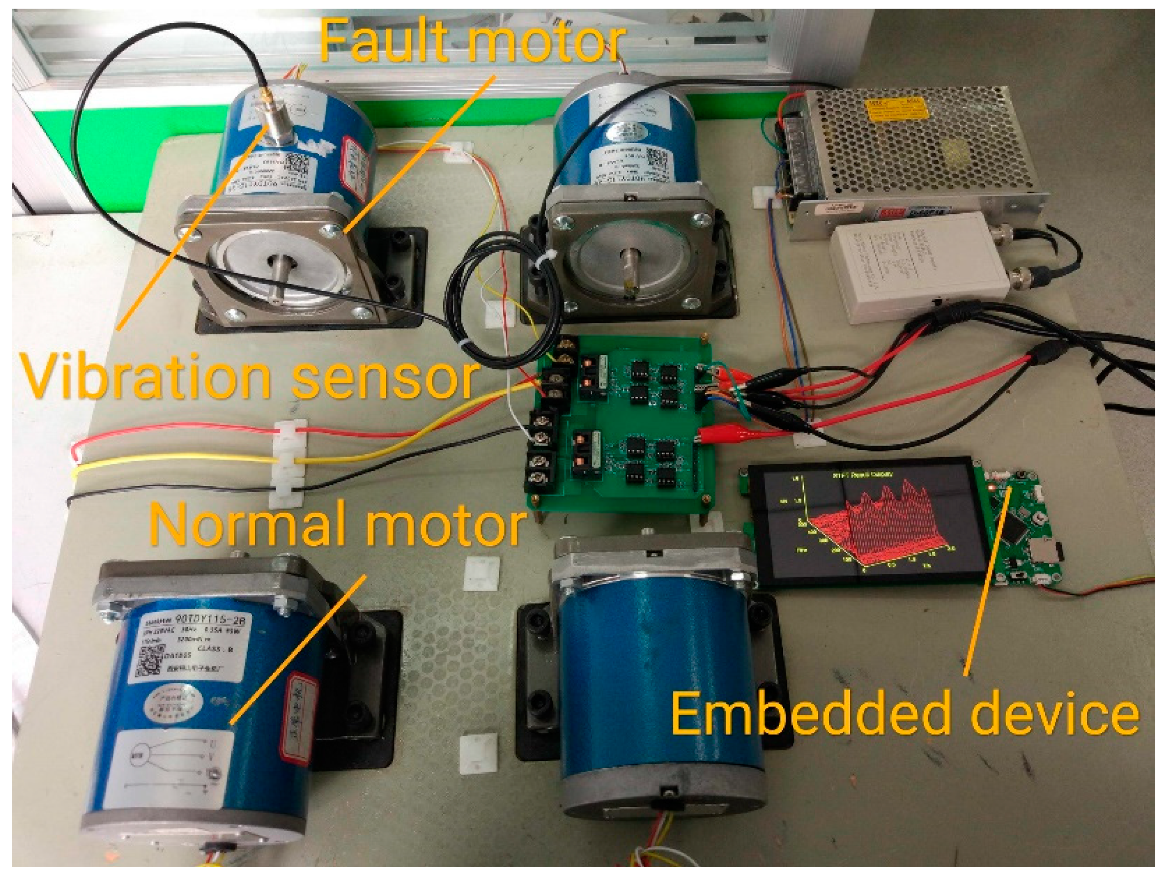
The experimental platform is shown in Figure 5. It consisted of two three-phase permanent magnet synchronous motors (PMSM), several current sensors, and a vibration sensor. The data collected by the sensors were uploaded to the embedded device.

Two permanent magnetic low-speed synchronous motors were used in the experiment. One was a normal motor and the other was a fault motor. The fault motor was artificially set to a 15% inter-turn fault in the stator. This PMSM had 26 poles and 12 stator slots, whose rated frequency and power were 50 Hz and 95 W, respectively.

The vibration signal was collected by a piezoelectric accelerometer, whose voltage sensitivity was 100 mV/g. The frequency response range of the accelerometer was 0.5 Hz–6000 Hz, and the maximum output signal of the accelerometer was 6 V. The sensor was attached radially to the housing of the motor.

3. Results

The proposed SMSG algorithm was applied to display the spectrograms of the fault diagnosis experiment. The experimental data was also used to carry out another test, which could verify the efficiency of the proposed SMSG algorithm, by comparing its results with that of the painter’s algorithm.

3.1. Vibration Signal Analysis

In this experiment, a motor was artificially set to 15% inter-turn short circuit fault of a single phase. The vibration signal was analyzed to extract the fault features. The time-domain waveforms of vibration signals are shown in Figure 6. It could be seen from Figure 6 that the amplitude of the fault motor vibration signal was much larger than that of normal motor, and that the vibration signal oscillated periodically.

Figure 7 shows the results of the power spectrum of the two vibration signals. In Figure 7, the fundamental frequency of the vibration signal, which was 100 Hz, was two times of the current signal, which was 50 Hz. Compared with the frequency spectrum of the normal motor, the amplitude of the fault motor was obviously increased at the fundamental frequency, which was 2 fs = 100 Hz. In addition, several high frequency harmonic components appeared in the vibration signal, located at the frequencies of 3 fs = 150 Hz, 4 fs = 200 Hz, 6 fs = 300 Hz, and 8 fs = 400 Hz.

The above is all that we could obtain from the Fourier Transform analysis in frequency domain. However, since the vibration signal was a time-varying signal, the STFT method could get more information from its spectrogram.

Figure 8 is the STFT spectrogram of the fault motor, obtained by MATLAB. The spectrogram drawn by an embedded device, based on the proposed SMSG algorithm is shown in Figure 9. It could be seen from Figure 8 and Figure 9 that the two results were very similar, which means that the proposed SMSG algorithm was correct.

From the front view of the spectrogram, it could be clearly seen that the amplitude of the 100 Hz frequency was very large, but the other Time-Frequency Distribution (TFD) components behind the 100 Hz frequency were invisible. Therefore, in order to observe the TFD more comprehensively, the back view spectrogram was needed.

The back view of the spectrograms of the fault motor and the normal motor are shown in Figure 10 and Figure 11, respectively. Since the amplitude of the normal motor was smaller than that of the fault motor, its spectrogram has been zoomed in for easy observation.

It could be seen from the 3D time-frequency spectrogram that the motors’ frequency components are very abundant, and the appearances of the spectrograms of the two motors, were distinct. If the stator winding of a motor broke down, it would cause magnetic field distortions in the air gap, which would generate electromagnetic forces and would finally lead to the radial vibration of the stator and the rotor. So, the characteristic of the motor vibrations would appear to be very different.

From Figure 10 of the fault motor, we can see that the amplitude of two frequency components, that is, 100 Hz and 200 Hz, exhibited a very significant periodic variation. However, the same frequency components of the normal motor, as shown in Figure 11, did not show this feature. This indicated that the two frequency components of 100 Hz and 200 Hz are varied with time, by a periodic shock, only in the fault state. It can be seen from Figure 10 that the period of this shock was approximately equal to 0.5 s, which meant that the changing frequency of the two frequency components was nearly 2 Hz.

According to the parameters of the motor, the speed of the revolution could be calculated by the following formula:

$$\begin{array}{l}n=\frac{60f_s}{p}=\frac{60\times 50}{26}\mathrm{r}/\min \\ \approx 115.4\mathrm{r}/\mathrm{m}\mathrm{i}\mathrm{n}\approx 2\mathrm{r}/\mathrm{s}\end{array}$$

(12)

Theoretically, from the result of Equation (12), the rotational frequency was 2 Hz, which was the same as the shock period that appeared in Figure 10. Therefore, it could be concluded that the fault motor was subjected to an impact force of 2 Hz, during each rotation process.

3.2. The Efficiency of the Spectrogram Mesh Surface Generation (SMSG) Algorithm

In order to verify the efficiency of the proposed SMSG algorithm, two display algorithms were carried out by Visual C++ language, on a PC. The painter’s algorithm and the SMSG algorithm were respectively employed to perform a 3D display under different mesh numbers. The elapsed time of the two algorithms is shown in Figure 12, where the consumed time is measured in milliseconds (ms).

It can be seen from Figure 12 that the time growth of the SMSG algorithm was very stable, and the time increment was not obvious. With the growing number of meshes, the time of the painter’s algorithm increased exponentially. The reason was that, in the painter’s algorithm, a lot of time was needed to calculate, compare, and sort the depth value of each mesh surface. However, in the SMSG algorithm, this kind of work was not needed and the points were directly taken from the vertex table, which saved considerable time. So the SMSG algorithm was very fast, even for a large number of meshes.

4. Conclusions

An effective mesh surface generation algorithm for the time-frequency spectrogram display was presented in this paper. The proposed method, SMSG algorithm, was based on the painter’s algorithm, which could solve the problem of a hidden surface removal in an accurate mesh surface generation. Then the SMSG was adapted to the special 3D displaying application of time-frequency analysis results. According to the characteristics of a joint time-frequency distribution matrix, the sorting calculation in the painter’s algorithm was omitted. The 3D graph was drawn directly in the sequential order of time array and the size order of frequency array.

The proposed algorithm was fast, clear, and simple, which meant that it could especially be used in embedded systems. The effectiveness and the practicality of the method were validated by an experimental motor test.