Humid environments can have chemical and physical effects on aircraft components, especially when condensation occurs due to temperature and humidity changes [
1]. For metal structures, the combined effect of humid air and other factors could cause chemical or electrochemical damage to the surface coating of structures [
2] leading to electrochemical corrosion of the metal underneath [
3,
4,
5,
6]. When exposed to a humid environment, structures made of composite materials can absorb moisture from the air, resulting in a variety of undesirable consequences such as expansion, stratification, and a reduction in strength [
7,
8,
9]. For airborne equipment, condensation and free water that occurs in humid environments could cause electrical short circuits [
10], blurring of optical lenses, surface mildew, and other problems. Moreover, humid environments give rise to a range of potential problems including changes in the friction coefficient, degradation of lubricants, faulty explosives, and sealing element aging, all of which could lead to mechanical failure of the aircraft [
11].
Military aircraft are parked on the ground for more than 95% of the time during service [
12], and the figure for civil aircraft is 65%. Most load-bearing structures (such as longerons, spars, ribs bulkheads, and stringers), rubber parts, and airborne equipment are located inside the aircraft and are therefore subject to long-term direct influences from the local environment of the bay. Thus, determining the local environmental characteristics of grounded aircraft is of the utmost importance in assessing the service life of internal components of the aircraft, preventing functional failures, and analyzing the causes of malfunctions [
13,
14].
Service environment spectra of components can be generated to assess the corrosion of aircraft parts in the laboratory [
15]. At present, the key factors that should be taken into consideration in the preparation of a service environment spectrum are the temperature, humidity, and corrosive media in the atmosphere [
16,
17,
18], which are roughly the same as the external environmental factors of the aircraft. If a relationship between the local environment inside the aircraft bay and the external environment can be established, the internal environment of the aircraft can be effectively simulated using existing methods [
18,
19], thus, the corrosion of internal parts can be assessed with sufficient accuracy.
A lot of effort has been placed on studying the local environment of aircraft. Zhang [
20] measured and statistically analyzed the temperature and humidity inside the tank of grounded aircraft. Jin et al. [
21,
22] classified the various bays into three types, namely open, semi-open, and closed, according to the local temperature and humidity data of the aircraft and established a regression model.
In previous work, we measured the local temperature of grounded aircraft, analyzed the temperature variation patterns of different bays, and proposed the structural coefficient and illumination coefficient as a means of describing the effects of the bay on the local temperature [
23]. Further, an aircraft local temperature model was established with the temperature measured from within a thermometer shelter as the independent variable. High precision of the model was validated by experiments showing the discrepancy between the predicted temperature and measured temperature to be less than 1.2 °C at all locations.
Based on the above studies, the local humidity of grounded aircraft is explored further in this paper, a local humidity model is established, and its accuracy is verified. The results presented herein are complementary to those previously published in a similar study, and together these studies lay the foundation for the preparation of a complete local environmental spectrum of the grounded aircraft [
23].
1. Measurement and Analysis of Local Humidity
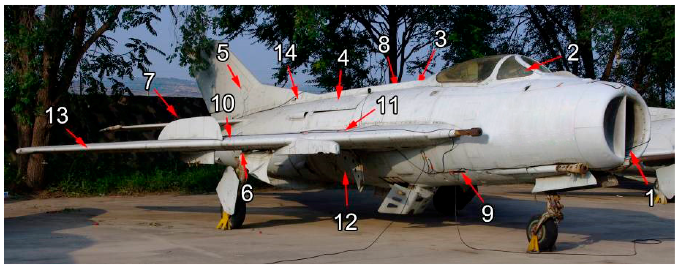
For this study, measurements of the local humidity of grounded aircraft (i.e., the humidity inside each structural bay of the aircraft) were carried out according to the previously reported method [
23]. The test aircraft used in this study was a retired fighter parked on a parking apron, without the protection of a shelter. To make up for the limitation of a single aircraft model, 14 measurement points were fitted inside the aircraft to study the influences of bay size, location, and structure, as well as different weather conditions, on local humidity. To make up for the limitation of a single geographic location, measurements were performed across an entire year such that the aircraft experienced large variations in the external environmental conditions. Since the focus of this study is on exploring the relationship between the local humidity of the bays and the external environment, and since most aircraft have similar bay structures (the retired aircraft is a small aircraft however bays of large aircraft, especially large fighter planes, are divided into smaller spaces by bulkheads and ribs, therefore the partial cabin size of large aircraft is comparable to the bay of a retired aircraft), the conclusions of this study can be widely applied to other aircraft models across other geographical regions. When studying different aircraft models in different geographic locations, the bay classification system along with the humidity model proposed in this paper, with modification to certain parameters, could potentially be used.
1.1. Measurement of Local Humidity
Temperature and humidity sensors (DW485N-A) were used. Errors in temperature measurements were less than 0.5 °C and errors in the relative humidity measurement were less than 4% relative humidity (RH; at 25 °C). Sensors were placed in the aircraft bays and the data was recorded every minute and transmitted to a computer via wires. To ensure measurement accuracy, a silicon sealing ring was applied to each wiring hole to prevent water from entering the bay and ensure it remained closed. In order to compare the variation patterns of temperature and humidity, humidity measurements in this study were conducted within the same 12-month period as the temperature measurements previously reported [
23].
A total of 15 local temperature measurement points were assessed. Fourteen were located inside the aircraft bay and one was located in the thermometer shelter outside the aircraft. The internal measurement locations are shown in
Figure 1.
The aircraft bays were classified into three types according to how closed or open they are: Open, semi-open, and closed [
22]. Measurement points 1, 6, 7, and 9 were located in the open bays, measurement points 4, 11, and 14 were in the semi-open bays, and measurement points 2, 3, 5, 8, 10, 12, and 13 were in the closed bays. Lastly, measurement point 15 was located outside the aircraft.
1.2. Results and Analysis
Similar to the reporting method previously described in reference [
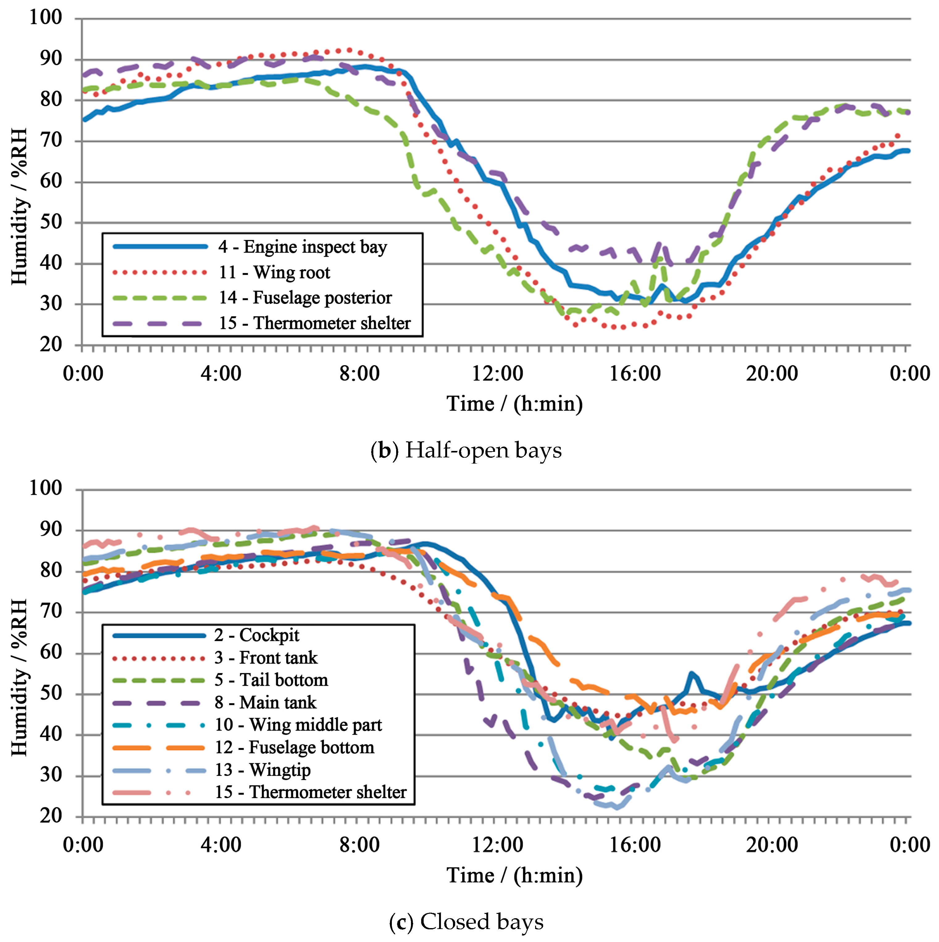
23], humidity data of the 15 measurement points was acquired throughout the day on 31 July 2013, which was taken as an example for this analysis. The data of each bay type (open, semi-open, or closed) was plotted, as shown in
Figure 2. To show the relationship between the humidity of each bay and the ambient humidity, the acquired humidity from within the thermometer shelter is also illustrated on the graphs presented in
Figure 2. On that day, the ambient humidity varied significantly within the range of 38.6 to 90.76% RH, and a light to moderate rain shower took place between 16:25 and 16:50, causing dramatic variations in humidity.
From the humidity curves, it can be observed that from 9:00 to 22:00, differences in humidity between measurement points existed, as suggested by the relatively large variation in the 15 humidity curves. The maximum difference in humidity can be observed at 14:50 when the highest humidity was measured at measurement point 12 as 28% RH higher than the lowest humidity measured at measurement point 13. Differences in humidity are relatively small during the nighttime, with a maximum difference of approximately 10% RH. The humidity measured inside the thermometer shelter was in the medium-to-high range among the other measurement points.
Large humidity differences can occur between different measurement points within the bays of the same open/closed state, as seen in the cases of the pair of measurement points 6 and 7 and pair of points 12 and 13. Humidity differences that occur between bays of the same open/closed state do not necessarily imply that the bay type has no influence on local humidity. This can be owing to three reasons. First, the vapor transmission process can be affected by the open/closed state of the bay. Second, the difference in local temperature as a result of differences in bay type can affect local humidity. Third, water can accumulate in a bay, which directly affects local humidity. A comparison with the previous study reveals that the difference in local humidity between bays of the same type is smaller compared to differences in local temperature [
23]. In other words, humidity is more closely related to bay type.
All bays underwent humidity changes due to the rain shower from 16:25 to 16:50, as indicated by the peaks on the curves during this period. However, the extent and length of the response varied from bay to bay. The rain shower caused the atmospheric humidity to increase by 7.7% RH. The largest increase in local humidity (13%) occurred at measurement point 14 (fuselage posterior), and the least change (2%) was observed at measurement point 3 (front tank). While the humidity changed almost immediately at most of the measurement points in response to the changes in atmospheric humidity after the rain shower started and reached a maximum when the rain stopped, the humidity response at measurement point 2 (cockpit) was approximately one hour later.
1.3. Relationship between Local Humidity and Local Temperature in the Bay
It can be seen from the humidity variation curves presented in
Figure 2 that the local humidity of the bay dropped from around 8:40 to 16:30 during the day. Between 16:30 and 8:40 the following day, the local humidity of the bay increased and became stabilized. Comparing the local humidity curves obtained in this study with the previously published local temperature curves [
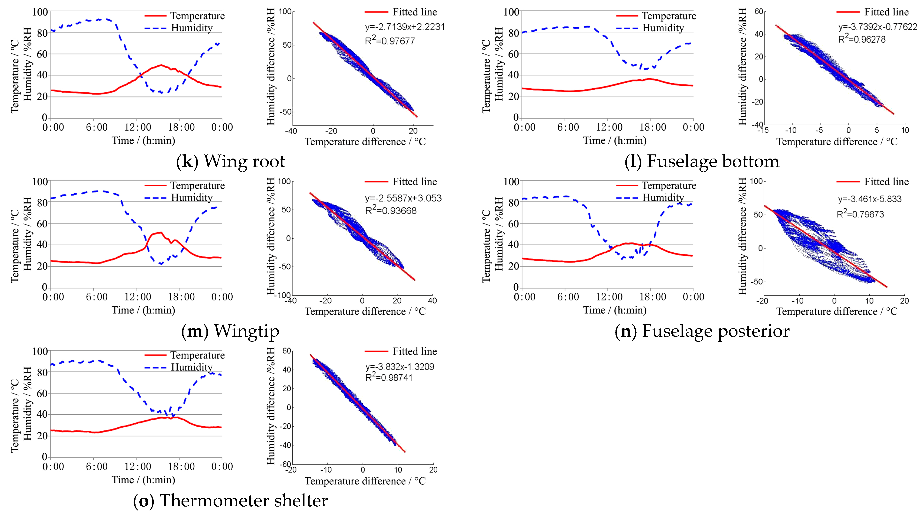
23] leads to the conclusion that the pattern of variation in local humidity is correlated to the temperature turning points. More specifically, major changes in local humidity always occur 40 min to 1 h after a major change in local temperature. Therefore, in order to determine the degree of correlation between the local humidity and local temperature, the temperature and humidity variation curves for each bay were plotted in the same graph, as shown in
Figure 3. The dotted lines represent humidity variations and the solid lines represent temperature. It can be seen from the graphs on the left side of
Figure 3 that there is a large negative correlation between the humidity and temperature variations. The humidity drops as temperature rises and increases as temperature drops.
To assess the influence of local temperature on the local humidity in the bay, temperature and humidity data were processed using the following formulae:
where
Tk and
Tk+l are the
k-th and
k+1-th temperature values of the bay and
hk and
hk+l are the
k-th and
k+1-th humidity values, Δ
Tkl is the discrepancy between the two temperature values separated by
l values, and Δ
hkl is the discrepancy between the two humidity values separated by
l values. Taking Δ
Tkl as the abscissa and Δ
hkl as the Y-axis, the graph shows the relationship between the humidity and temperature variations in the bay. The data was then analyzed in MATLAB to obtain the graphs shown on the right side of
Figure 3. The scatter plots correspond to values of Δ
Tkl and Δ
hkl, and the solid lines were fitted to the data using the least squares method based on temperature and humidity variation patterns. It can be seen that there is a large negative correlation between the rate of change of the local humidity and temperature in the bay.
When the value of
l in Equation (1) is zero, then Δ
Tkl and Δ
hkl are both zero, which means that in theory, the lines of best fit, should pass through point (0, 0). The theoretical model of the fitted line should be a proportional model with a negative slope, that is
where
qi is the slope and expresses the relationship between the rates of change of temperature and humidity of the
i-th bay. Since there can be a multitude of influencing factors affecting the local humidity of the bay in real-world scenarios, some discrepancy will always exist between the actual fitting formula and the theoretical model, which is simply a linear model with an intercept value. Since the intercept value in the fitting formula is not large, it was not taken into account in the actual fitting formula used in this study, and instead “coarse granularity principle” for studying environmental spectrum was followed [
24].
Figure 3 only shows the relationship between the local temperature and local humidity in the bay and the rate of change during a single day. To reveal a more general pattern, temperature and humidity data of 30 randomly selected days within one year were selected and processed using Equation (1), with the aim of fitting a relational expression to describe the rates of change of temperature and humidity for each bay. Statistical analysis revealed that the slope of the relational expression of the rate of change of temperature and humidity can vary from one day to another. The maximum difference between slopes can reach −2.0% RH/°C, that is, when the average local temperature of a bay rises by 1 °C, the difference between in humidity measured on different days decreases and can reach up to 2.0% RH. However, when the temperature and humidity variations measured at the measurement point 15 (thermometer shelter) are included in the analysis, a new conclusion emerges. Regardless of date, the ratio of the slope of the relational expression of the rate of change of temperature or humidity to that of the thermometer shelter is usually a fixed value. In other words, if the slope of the relational expression of the rate of change of temperature and humidity of a bay is
qi, and the slope of the thermometer shelter is
q0, the value of
qi/q0 is only related to the position and structural type of the bay. Here,
pi =
qi/
q0 is called the humidity characteristic coefficient (HCC) of the bay and
qi is a dimensionless quantity that reflects the responsiveness of the local humidity of the bay to temperature changes. The temperature and humidity data of 30 days were statistically processed. Average
and variance σ
2 values of
pi are listed in the
Table 1.
It can be seen that the average values of all but measurement point 15 (thermometer shelter) are less than 1. This indicates that the |qi| values of all bays are smaller than |q0|, which means that the responsiveness of local humidity to temperature changes is smaller in all bays than in the thermometer shelter. This is mainly attributed to the closed nature of the bays. The more closed the bay, the lower the value of .
Since the sample size for calculating
values in
Table 1 is large and the variance σ
2 is small, the HCC
pi of each bay is given a
value, listed in
Table 1.
2. Establishing the Aircraft Bay Humidity Model
Based on the above analysis on the measured humidity values and the relationship between local temperature and humidity in the bay, it can be concluded that humidity does not vary much during the nighttime. The nighttime local humidity can be determined using the ambient humidity (measured in the thermometer shelter) and the structure coefficient
mi (previously defined in reference [
23] and reflects the responsiveness of the local temperature of the bay to the ambient temperature, which is only related to the type of bay). According to this, humidity values during the daytime can be obtained using local temperature values of the bay and the slope of the relational expression describing the rate of change of temperature and humidity
qi.
Assuming that the humidity value of the
i-th bay at the
j-th moment of the day is
hij, then the temperature value is
Tij, and the temperature and humidity values measured at the thermometer shelter are
T0j and
h0j, respectively; the bay structure coefficient is
mi; the illumination coefficient is
si (provided in reference [
23] and reflects the responsiveness of the bay to sunlight); and the bay HCC is
pi.
Since the nighttime temperature model of the bay is
Tij = T0j + mi [
23], and the temperature differences between the different bays at night is only related to the bay structure coefficient
mi (that is,
mi can be regarded as a coefficient reflecting the temperature difference between bays at night), the first measured humidity value
hi0 at time 0:00 every day can be approximated by the following formula:
where
h00 is the first humidity value measured at the thermometer shelter at 0:00.
According to Equations (1) and (2),
Therefore, if the first humidity value
hi0 of the bay can obtained, the bay humidity value can be calculated based on the bay temperature value, as follows:
According to reference [
23], the mathematical expression of the local temperature model of the aircraft bay is
where
Tij is the local temperature of the
i-th bay,
si and
mi are the illumination coefficient and structural coefficient of the bay, respectively,
T0j is the ambient temperature (measured at the thermometer shelter),
Tt is the ambient temperature when the sunshine starts to take effect (normally the ambient temperature measured 2 h after sunrise).
According to Equations (3) and (6), Equation (5) can be rewritten as
where h
00,
h00,
T0j, and
T00 are values measured at the thermometer shelter;
mi,
si and
pi are parameters of the bay (which are known quantities based on real-world scenarios);
q0 is the amount of fitting obtained by applying the temperature and humidity values measured at the thermometer shelter to Equations (1) and (2).
According to Equation (5), the humidity at the thermometer shelter is
Therefore, Equation (7) can also be rewritten as
In real-world applications,
piq0 in Equation (9) can be approximated as −3, then the above formula becomes
Both Equation (7) (model 1) and Equation (10) (model 2) can be used as predictive models for the local humidity of the bay. Equation (10) is simpler and there is no need to calculate q0 for each variation of temperature and humidity measured at the thermometer shelter. Therefore, Equation (10) is suitable for estimating the local humidity of the bay. Equation (7) is more accurate, the computational requirements are much higher, and dedicated computer software is needed.
3. Classification of Aircraft Bay Structures Based on Local Humidity Characteristics and Ranges of Model Parameters
Based on the bay temperature model, described by Equation (6), the bay humidity characteristic coefficient pi, a new parameter, is introduced into the bay humidity model. This parameter reflects the sensitivity of the bay humidity to temperature changes and is a quantity related to the bay type. Therefore, it is feasible to classify the aircraft bay structures according to differences in the bay HCC pi.
The
pi values of different bays are provided in
Table 1 and the bays are classified into three types according to the local humidity characteristics: Type I {no. 2, 3, 8, and 10}, type II {no. 13, 5, 6, 11, and 4}, and type III {no. 9, 1, 12, 14, and 7}. The key model coefficient values for each bay type are listed in
Table 2.
It can be seen that the bay structure classification based on humidity characteristics is related to the open/closed state of the bay. The results of the humidity-based bay classification differ from the results of the temperature-based bay classification previously reported [
23]. This is largely because the local temperature and local humidity of the same bay vary in a different way in response to the changing conditions.
The HCC pi of the type I bays is in the range of 0.409–0.694. Type I bays are closed with good sealing and large spaces. The HCC pi values are larger for type I bays with relatively poor sealing and smaller spaces.
The HCC pi of type III bays is in the range of 0.943–0.994. These bays are characterized by good ventilation and lower bay temperatures. Bays located in the lower part of the aircraft, and therefore the least influenced by sunlight, are type III. The HCC pi values are higher for type III bays with relatively good ventilation and lower temperatures.
The rest of the bays belong to the type II group, with a HCC pi ranging from 0.772–0.913. Generally, the main characteristic of these bays is that temperatures are moderate. Some open or semi-open bays have a relatively high temperature, and closed bays with poor sealing or small spaces fall into this category. The HCC pi values are larger for type II bays with relatively good ventilation, low temperatures, and large spaces.
The bay structure coefficient mi and illumination coefficient si are related to the bay temperature characteristics. The structure coefficient mi of the bays whose outer surface is exposed to direct sunlight ranges from −0.8 to 0.5, and sunshine coefficient si ranges from 1.56 to 1.86. Bays located in the inner part of the aircraft are therefore only indirectly influenced by sunlight with structure coefficient mi in the range of −0.8–0.5 and sunshine coefficient si ranging from 1.40 to 1.53. Bays located in the lower part of the aircraft, and therefore least influenced by sunlight, have a structure coefficient mi in the range of 2.4–3.0, and their sunshine coefficient si ranges from 0.86~1.02. At night, the sunshine coefficient si of every bay is assigned a value of 1.
4. Testing of the Aircraft Bay Humidity Model
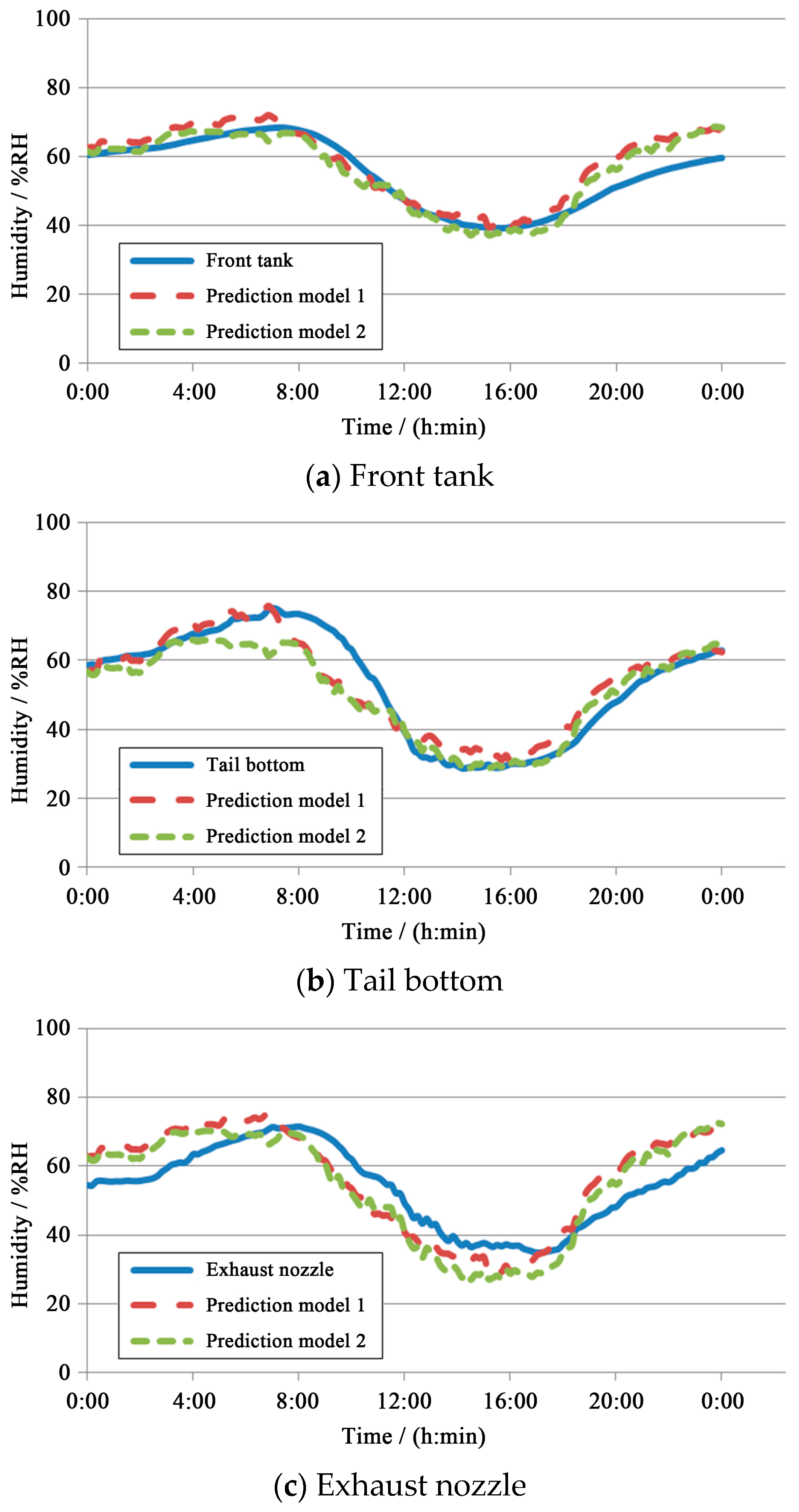
To verify the accuracy of the bay humidity model, the humidity dataset of a specific day was selected and used to produce two sets of bay humidity prediction values using model 1 based on Equation (7) and model 2 based on Equation (10). Predicted values were compared with measured values. The humidity dataset of a randomly selected day was processed. Two humidity variation curves were plotted for each of the selected bay groups using the model prediction data and measured data, as shown in
Figure 4. The selected group of bays were: Kerosene tank (measurement point 3, closed, type I), tail bottom (measurement point 5, closed, type II), exhaust nozzle (measurement point 7, open, type III), where
m3 = 0.8,
s3 =1.40,
p3 = 0.594;
m5 = 0.5,
s5 = 1.48,
p5 = 0.813;
m7 = 2.4,
s7 = 0.93,
p7 = 0.994;
t00 = 18.35 °C,
h00 = 63.92% RH,
q0 = −2.9875% RH/°C (
si = 1 at night).
A statistical analysis was performed on measured humidity values at three measurement points and the predicted humidity values produced by the two models. Results are listed in
Table 3.
The correlation coefficient is
where
hij is the
j-th humidity value of the
i-th bay obtained according to the humidity model;
is the measured
j-th humidity value of the
i-th bay;
n is the number of data points measured at one measuring point,
n = 24 h × 60 min/h × 1 min
−1 = 1440;
is the average humidity of the
i-th bay.
From
Table 3, it can be observed that the humidity values predicted by the model are in good agreement with the measured humidity values, with an average deviation less than or equal to 7.3% RH. Given the current practice of preparing an environmental spectrum in which normally only a humidity of 60% RH or higher is considered [
14] and every 10% RH is converted into a standard humid air action time, the two humidity prediction models were established and may be able to serve as effective tools in the preparation of local environmental spectra of bays.
5. Conclusions
- (1)
A high negative correlation was found between the rate of change of humidity and rate of change of temperature of the bay. The ratio of the slope of the relational expression of the rate of change of temperature and humidity qi of a particular bay to rate of change associated with the thermometer shelter q0 is a fixed value pi, called the bay humidity characteristic coefficient. This value reflects the dimensionless response of the local humidity of the bay to local temperature changes.
- (2)
Different aircraft bays in the open/closed state may differ in terms of humidity, however, sealing has a major influence on local humidity. Better sealing of the bay will result in lower values of the corresponding HCC pi and the overall humidity level will also be lower.
- (3)
Two bay local humidity models were established by using the ambient humidity and temperature (measured at the thermometer shelter) as independent variables and incorporating a number of influential parameters such as the structural coefficient mi, illumination coefficient si, and HCC pi.
- (4)
Values of HCCs of different bays were determined through statistical analysis and, based on this, the aircraft bays were classified into three types. A comparison between measured data and model data suggests the average deviation of the model proposed in this paper is less than or equal to 7.3% RH.


