Fault Diagnosis of Rolling Bearings Based on Improved Fast Spectral Correlation and Optimized Random Forest

Abstract

Fault diagnosis of rolling bearings is important for ensuring the safe operation of industrial machinery. How to effectively extract the fault features and select a classifier with high precision is the key to realizing the fault recognition of bearings. Accordingly, a new fault diagnosis method of rolling bearings based on improved fast spectral correlation and optimized random forest (i.e., particle swarm optimization-random forest (PSO-RF)) is proposed in this paper. The main contributions of this study are made from two aspects. One is that an improved fast spectral correlation approach was developed to extract the fault features of bearings and form the feature vector more effectively. The other is that an optimized random forest classifier was developed to achieve highly accurate identification by exploiting particle swarm optimization to select the best parameters of random forest (RF). In the presented method, improved fast spectral correlation was first utilized to analyze the raw vibration signal caused by a faulty bearing to obtain the enhanced envelope spectrum. Then, the amplitudes of the four characteristic cyclic frequencies (i.e., the rotating frequency, the characteristic frequency of outer-race fault, the characteristic frequency of inner-race fault, and the characteristic frequency of rolling element fault) exhibited in the enhanced envelope spectrum were selected to form the feature vector. Finally, the PSO-RF method was introduced for identifying and classifying bearing faults. The experimental investigations demonstrate the proposed method can accurately identify bearing faults and outperform other state-of-art techniques considered.

1. Introduction

As an important supporting element, rolling bearings are widely used in various rotating machinery systems, such as wind turbines, aero engines and internal combustion engines. A minor bearing fault may affect the operation of the whole rotating machinery. Moreover, bearing faults can cause huge economic losses or even casualties [1,2,3]. With the rapid emerging and popularization of the Internet and the Internet of things, big data have brought revolutionary challenges and disruptive innovation to traditional information technology. Fault diagnosis has also entered the era of “big data” and fault recognition is an important part of it.

The factors that cause bearing failure are numerous. The main causes of bearing failure include manufacturing and assembly faults which lead to vibrations dominated by out-of-balance shaft response and cage related frequencies [4]. Other modes of failure of bearings are initiated by contact conditions. Some are due to loss of the preload or interference fitting, which are known as the variable compliance effect [5]. Another major mode of failure in bearings is lubrication issues, lack of which can lead to wear, excessive friction and heat generation and scuffing. Finally, the worn rolling and sliding surfaces cause vibration, by which time any solution to the problem would be too late [6,7,8,9].

Fault feature extraction and fault classification are two important aspects of bearing fault diagnosis. Using an effective fault feature extraction method to establish the fault feature vectors that fully reflect the fault information and selecting an advanced classifier to train and recognize the feature vectors are important to ensure the high precision of fault diagnosis. Many researches have been carried out on fault feature extraction of bearings. Wavelet packet decomposition was used to eliminate the noise of the signal and the fault features were extracted by ensemble empirical mode decomposition (EEMD) in Reference [10]. Successive wavelet decomposition techniques have also been used to focus on particular band of frequencies by obtaining the run-out wave attributed to particular features caused by the indicated sources, such as cage slipping, out-of-balance rotor rotation, etc. [11]. Gao et al. [12] combined the time frequency distribution and the non-negative matrix factorization to enhance the bearing fault characterization. Jiang et al. [13] used the singular value and ratios of neighboring singular values to extract the fault features. In Reference [14], bearing fault features were extracted via singular spectrum analysis. Li et al. [15] utilized the hierarchical fuzzy entropy and Laplacian score to extract the fault signatures of bearings. Zhou et al. [16] proposed a neighborhood component analysis based feature extraction approach. Liu et al. [17] proposed a method that combines Hilbert Huang transform (HHT) and singular value decomposition (SVD) to obtain the fault features of bearings. Cheng et al. [18] proposed an effective fault feature extraction approach by combining empirical mode decomposition (EMD) and SVD. In Reference [19], multi-scale permutation entropy (MPE) was used to extract fault features. In Reference [20] a fault feature extraction method based on EEMD, and multi-scale fuzzy entropy was proposed. These developed approaches are of great significance to fault diagnosis. However, some of them are proposed based on the signal decomposition methods, such as EMD, EEMD and wavelet decomposition. The EMD- and EEMD-based methods have modal aliasing problems which may affect the final identification results. A major limitation for the wavelet-based methods is that the analysis results are affected by the selection of wavelet basis functions. How to select wavelet basis functions adaptively is a difficult problem. Some other approaches belong to SVD and entropy based methods, whose effectiveness is easily affected by the parameter setting. In recent years, the cyclostationary theory plays an important role in the fault feature extraction of rotating machinery and it is conducive to improve the diagnosis results of rolling bearings and gears. In Reference [21], the minimum entropy deconvolution-spectral kurtosis (MED-SK) approach and cyclostationary (CS)-based approaches were investigated and compared. The results show that the CS-based approaches are more superior in detecting the early weak faults. Spectral correlation (SC) is one of the most effective CS-based approaches. Contrary to classical spectral analysis methods, spectral correlation can reveal the non-stationary characteristics of the analyzed signals. Therefore, it shows advantages for detecting bearing faults [22,23,24]. The averaged cyclic periodogram (ACP) has been the most popular and widely used estimator of SC for bearing fault failure detection [25]. In Reference [26], the averaged cyclic periodogram was combined with hidden markov model to diagnose the fault of rolling bearings. Antoni investigated the spectral correlation analysis of bearing signals thoroughly and pointed out the spectral correlation method is very suitable for detecting bearing fault signatures in Reference [27]. However, traditional SC techniques have low computational efficiency. Accordingly, Antoni proposed the fast spectral correlation (Fast-SC) method [28], which is a novel spectral correlation estimation method. The Fast-SC method not only has the advantages of spectral correlation, but also overcomes the shortcomings of high computational cost. However, the original signals of rolling bearings often contain many noise components and the fault features may be submerged in noise components. In the presence of noise and interference signals, the fast spectral correlation and enhanced envelope spectrums obtained by using Fast-SC always have interference frequencies.

Similarly, fault classification plays a key role in fault diagnosis of rolling bearings. Traditional fault classification methods including: back propagation (BP) neural network, artificial neural network (ANN), deep belief network (DBN), continuous hidden Markov model (CHMM), support vector machine (SVM), genetic algorithm (GA), adaptive fuzzy neural network (ANFIS), and extreme learning machine (ELM). BP neural network is a multilayer feed forward neural network. The prediction results are derived through forward deduction [29]. However, BP neural networks have the disadvantages of slow learning speed and low accuracy. ANN relies on the complexity of the system to achieve the purpose of processing information by adjusting the interconnected relationships among a large number of internal nodes and has the ability to learn and adapt itself. However, ANN has the possibility of overfitting data [30]. DBN is a continuous learning process which is layer by layer. In Reference [31], the accuracy and robustness of DBN is proved, but DBN has the shortcomings of computational complexity. CHMM is a double stochastic process, which has a hidden Markov chain of certain state numbers and a set of random functions. In Reference [32], CHMM was utilized to classify the faults and the results show that unreasonable parameter settings may affect the accuracy rate of CHMM. The learning strategy of SVM is to maximize the interval, which can eventually be transformed into a solution of a convex quadratic programming problem eventually. In Reference [33], EMD was used to decompose the signal into intrinsic mode functions (IMFs) and the fault feature was extracted by HHT. Finally, the fault features were input into SVM for recognition. SVM has good generalization ability, but it needs strict adjustment of kernel parameters and cannot solve multi-level problems effectively. In Reference [34], GA and SVM were combined to recognize the pattern of rolling bearing. In Reference [35], the time-frequency matrix of rolling bearing signal was calculated to extract fault feature and ANFIS was utilized to classify the pattern of rolling bearing fault. ELM uses random weights between the hidden layer and the input layer in the forward neural network. A method of destructive or adding regular terms is used to solve the output weights in the final output layer to achieve regression or classification [36,37,38]. In Reference [39], ELM was used for identification of bearing faults. Although ELM is fast and has strong generalization ability, it is limited by a hidden danger of fitting. Random forest (RF) is an advanced classifier. Training of RF is fast and easy to parallelize and it can handle data with high dimensions [40]. Therefore, RF is an effective and frequently used classifier for classifying bearing faults. In Reference [41], ReliefF ranking was used to rank the fault features obtained by calculating the statistical characteristics of the signal in the time domain and random forest was further used to identify bearing faults. In Reference [42], Wang extracted the fault features of bearings by using the wavelet packet decomposition and the classification was completed by RF. In Reference [43], an intelligent fault diagnosis approach was presented with the combination of ensemble empirical mode decomposition and RF. In Reference [44], variational mode decomposition was combined with autoregressive model parameters to extract the fault features and RF was used for pattern recognition. The analysis results show that RF has a higher accuracy compared to SVM, genetic algorithm-SVM (GA-SVM) and particle swarm optimization-SVM (PSO-SVM). However, RF is a parameterized classifier and the selection of the parameters of random forest will affect the accuracy of classification.

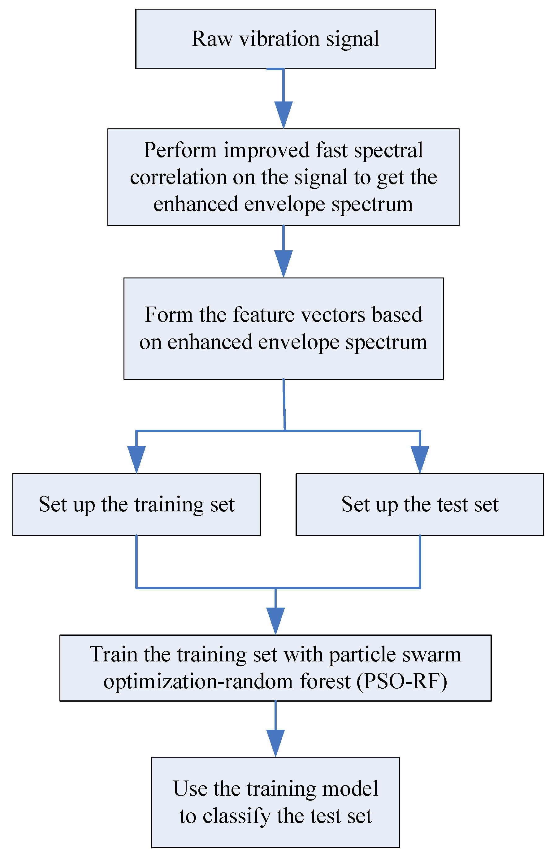
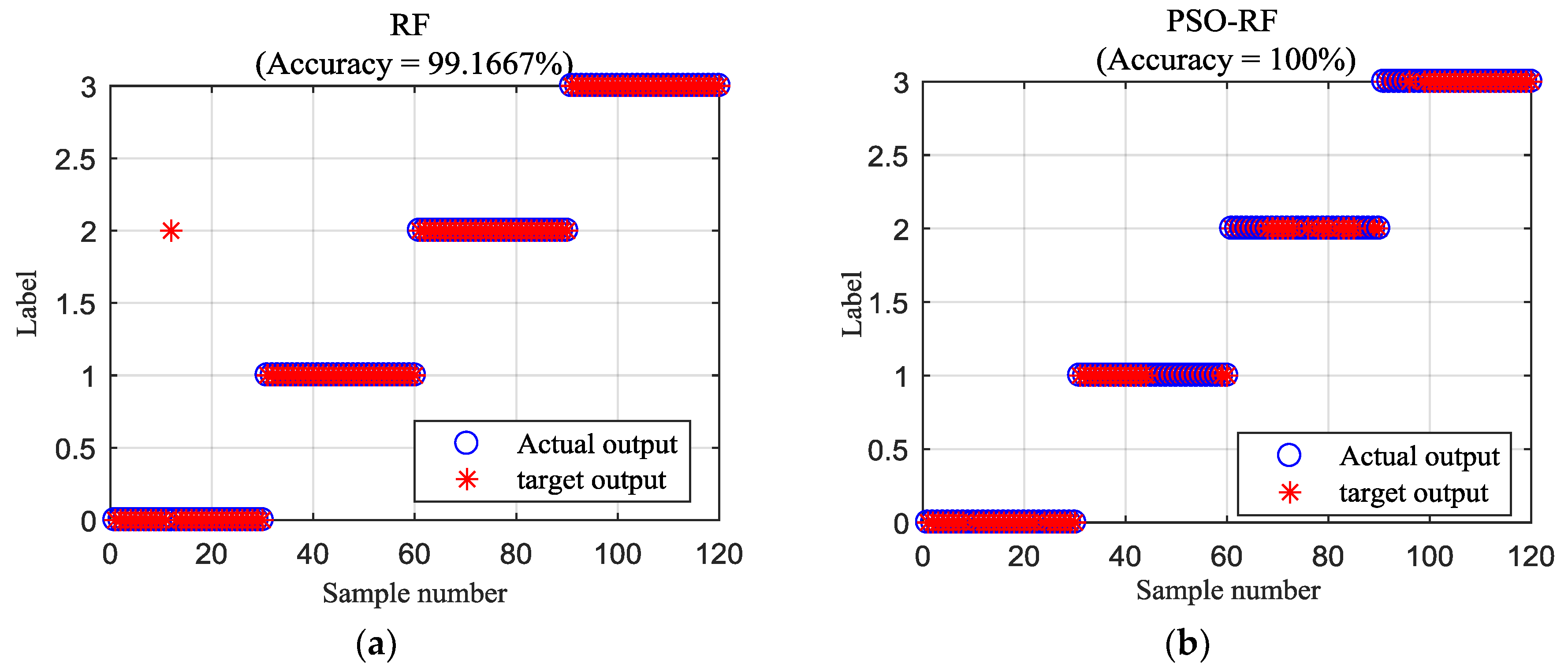
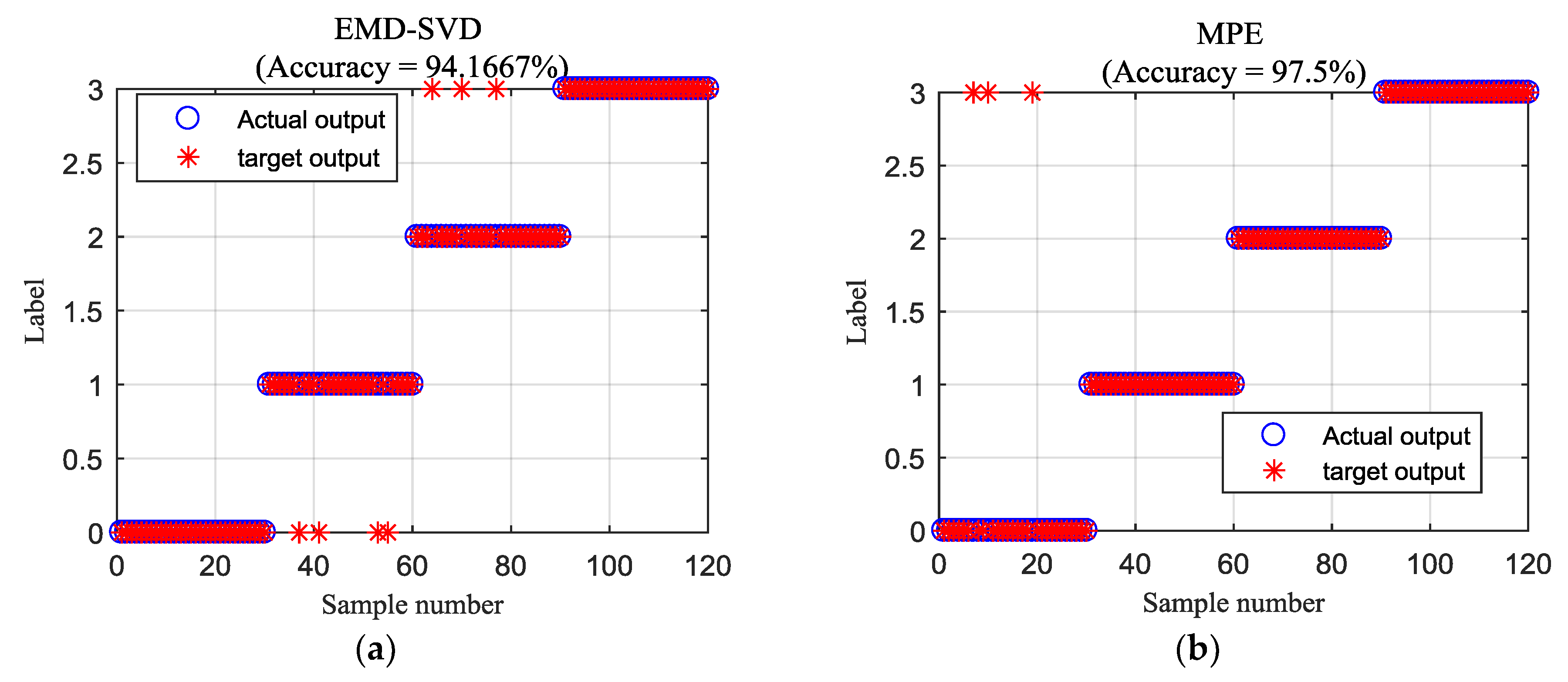
Considering that the fast spectral correlation is an advanced fault feature extraction technique and the RF is an excellent classifier. The main work of this paper was conducted on the basis of the fast spectral correlation and RF. To complete the accurate fault diagnosis of rolling bearings, an improved fast spectral correlation approach was proposed in this paper by introducing the kurtosis weighting to effectively decrease the effect of noise and highlight the fault characteristics. Moreover, a particle swarm optimization-random forest (PSO-RF) classification algorithm was proposed, which can adaptively optimize the parameters and improve the classification accuracy of RF. On the basis of the advantages of the improved fast spectral correlation and PSO-RF, a fault diagnosis method for rolling bearings was proposed with the combination of improved fast spectral correlation and PSO-RF in this work. The improved fast spectral correlation was firstly employed to extract the fault feature vectors of the faulty bearings. Then, the state classification of rolling bearings can be accomplished by training and testing the obtained fault feature vectors using the PSO-RF classifier.

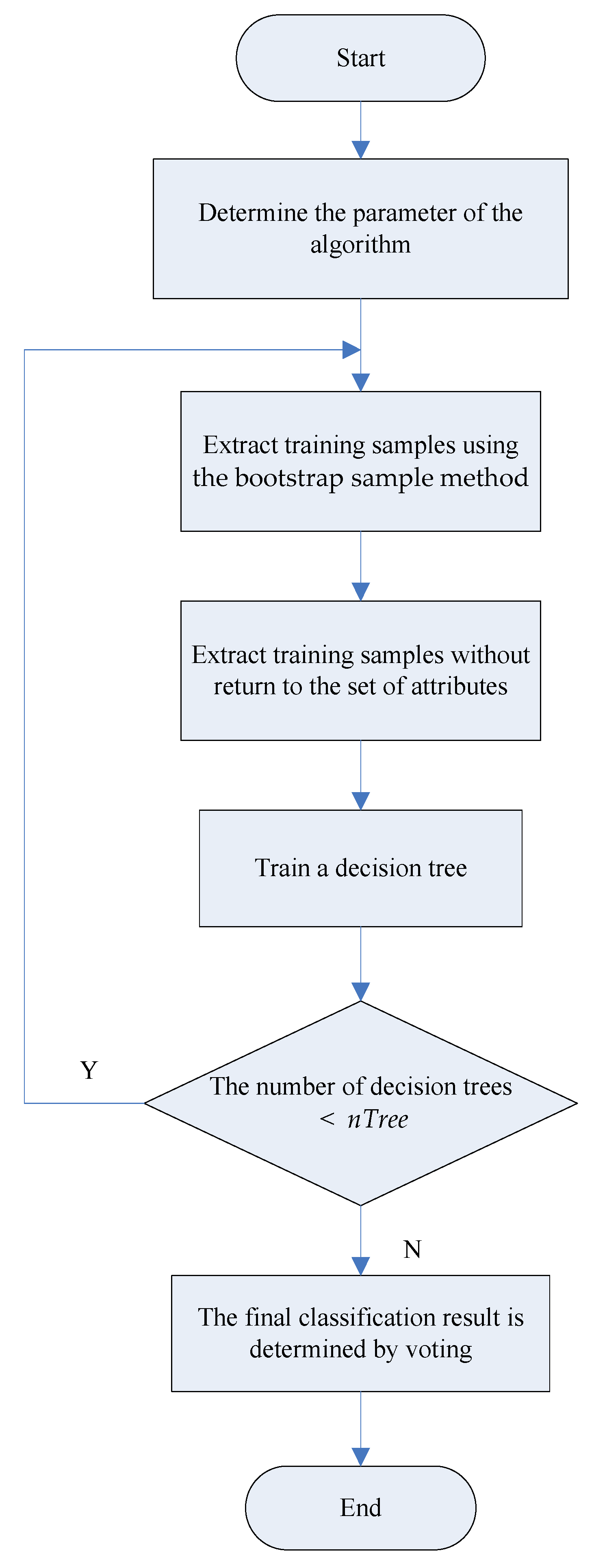
This paper is structured as follows. In Section 2, an approach of fault feature extraction based on the improved fast spectral correlation method is given briefly. Section 3 describes the details of random forest based on particle swarm optimization. Section 4 introduces the framework of the proposed method. In Section 5, the experiments are presented to investigate and validate the proposed method for state recognition of rolling bearing. Finally, conclusions are drawn in Section 6.

2. Fault Feature Extraction Based on Improved Fast Spectral Correlation

2.1. Brief Introduction of Fast Spectral Correlation

Let x(t_n) be a cyclostationary signal, its spectral correlation is defined as:

$$S{C}_x(\alpha ,f)=\frac{1}{F_s{}^2}{\displaystyle \sum _{n=-\infty }^{\infty }{\displaystyle \sum _{\tau =-\infty }^{\infty }{R}_x(t_n,\tau )e^{-j2\pi \alpha n\frac{1}{F_s}}}}{e}^{-j2\pi f\tau \frac{1}{F_s}},$$

(1)

where F_s is the sampling frequency, t_n denotes the time instants which can be calculated as t_n = n/F_s, R_x(t_n, τ) represents the cyclic autocorrelation function of x(t_n), τ indicates the time delay, α denotes the cyclic frequency and f represents the frequency.

The spectral correlation is a two-dimensional Fourier transform of two frequency variables, which reflects the power distribution of the signal relative to the frequency and the cyclic frequency. The power corresponding to the cyclic frequency α distributed along the line of the parallel frequency f.

In order to reduce the computational cost and improve the efficiency of spectral correlation, a fast spectral correlation method based on short time Fourier transform was proposed in Reference [28].

The short time Fourier transform (STFT) of the signal x(t_n) is described as follows:

$$X_{STFT}(i,f_k)={\displaystyle \sum _{n=0}^{N_w-1}x[iR+n]w[n]e^{-j2\pi n\frac{f_k}{F_s}}},$$

(2)

where N_w represents the window length of STFT, R represents the block shift in STFT; w[n] is the function of time index n; x[n] is the abbreviated form of x(t_n), f_k denotes the k-th discrete frequency and f_k = kΔf, Δf represents the frequency resolution, which has the expression of Δf = F_s/N_w.

Equation (3) shows the phase-corrected STFT [28]:

$$\begin{array}{cc}\hfill X_w(i,f_k)& ={\displaystyle \sum _{n=0}^{L-1}x[n]w[n-iR]e^{-j2\pi n\frac{f_k}{F_s}}}\hfill \\ & =X_{STFT}(i,f_k)e^{-j2\pi iR\frac{f_k}{F_s}}\hfill \end{array},$$

(3)

where X_w (i, f_k) denotes the complex envelope of signal x(t_n) at iR/F_s, whose center is f_k and bandwidth is Δf. ${\left|X_w(i,f_k)\right|}^2$ represents the energy flow in the frequency band.

Then the cyclic spectrum based on STFT is defined as [28]:

$$S_x(f,\alpha )=\frac{F_s}{L}{X}_w(f)X_w{(f-\alpha )}^{*},$$

(4)

where L is the length of signal x(t_n).

Assume that f = f_k = kΔf and α = pΔf + δ, it can be deduced that f − α = f_k − α ≈ f_k−p and α ≈ pΔf.

Applying these results to Equation (3), it comes that [28]:

$$X_w(i,f_k-\alpha )\approx X_w(i,f_{k-p})e^{j2\pi (\frac{\alpha }{F_s}-p\frac{\Delta f}{F_s})(iR+N_0)}.$$

(5)

where p is index of STFT frequency closest to a given cyclic frequency α, δ is residue.

Insert Equations (5) and (3) into Equation (4), the following Equation is obtained [28]:

$$\begin{array}{cc}\hfill S_x(\alpha ,f_k;p)& =\frac{1}{K{\Vert w\Vert }^2{F}_s}{\displaystyle \sum _{i=0}^{K-1}{X}_w(i,f_k)}{X}_w{(i,f_{k-p})}^{*}{e}^{-j2\pi (\frac{\alpha }{F_s}-\frac{p}{N_w})(iR+N_0)}\hfill \\ & =\frac{1}{K{\Vert w\Vert }^2{F}_s}\underset{i\to \alpha }{DFT}\left\{X_{STFT}(i,f_k)X_{STFT}{(i,f_{k-p})}^{*}\right\}{e}^{-j2\pi N_0(\frac{\alpha }{F_s}-\frac{p}{N_w})}\hfill \end{array},$$

(6)

When p = 0, the period of x(t_n) is T and its frequency α is 1/T. The energy flow will flow periodically in the band [f_k − Δf/2, f_k + Δf/2]. When p ≠ 0, X_w(i, f_k)X_w(i, f_k−p)^* represents the energy flow between band [f_k − Δf/2, f_k + Δf/2] and band [f_k−p − Δf/2, f_k−p + Δf/2].

The definition of fast spectral correlation is given as follows [28]:

$$S_x^{Fast}(\alpha ,f)=\frac{{\displaystyle \sum _{p=0}^p{S}_x(\alpha ,f;p)}}{{\displaystyle \sum _{p=0}^p{R}_w(\alpha -p\Delta f)}}{R}_w(0),$$

(7)

where $R_w(\alpha )={{\displaystyle \sum _{n=0}^{N_w-1}\left|w\left[n\right]\right|}}^2{e}^{-j2\pi (n-N_0)\frac{\alpha }{F_s}}$ denotes the kernel function and $R_w(0)={\Vert w\Vert }^2$.

The function of fast spectral correlation can be derived as follows [28]:

$${\gamma }_x(\alpha ,f)=\frac{S_x(\alpha ,f)}{\sqrt{S_x(f)S_x(f-\alpha )}}.$$

(8)

The enhanced envelope spectrum is defined as [28]:

$$S_x^{EES}(\alpha )={\displaystyle {\int }_{f_1}^{f_2}\left|{\gamma }_x(\alpha ,f)\right|}df.$$

(9)

2.2. Improved Fast Spectral Correlation

The signal of a faulty bearing is characterized by periodic impacts, which contains multiple harmonics in the spectrum and has a wide frequency characteristic. When the raw vibration signal is directly analyzed by fast spectral correlation, there may be many interference components in the obtained enhanced envelope spectrum around the characteristic cyclic frequencies. In order to extract the modulation information effectively, the kurtosis weighting was introduced to the fast spectral correlation analysis. Kurtosis is the fourth order of amplitude. It is sensitive to signals with larger amplitude and can play a role of energy amplification. The kurtosis was calculated for each column of the fast spectral correlation matrix and a greater weight was given for a bigger kurtosis. The modulation capacity of the cyclic frequency corresponding to the column can be effectively estimated. Therefore, a fast spectral correlation method based on kurtosis weight was proposed to enhance the fault features of bearings.

The specific steps of the improved fast spectral correlation method are as follows.

(1) Calculate the fast spectral correlation $S_x^{Fast}(\alpha ,f)$ of the original signal and calculate the kurtosis values of each column of $S_x^{Fast}(\alpha ,f)$ [45]:

$$\mathrm{KA}(\alpha )=\mathrm{mean}\left\{{[S_x^{Fast}(\alpha ,f)]}^4\right\}.$$

(10)

(2) Calculate the weighting factor KA’(α) based on Equation (11). The weighting factor reflects modulation ability of the modulation frequency. If the factor is greater, the modulation effect corresponding to this frequency in the original signal is stronger. Conversely, the modulation effect is weaker.

$$\mathrm{KA}\prime (\alpha )=\frac{\mathrm{KA}(\alpha )-\min \left[\mathrm{KA}(\alpha )\right]}{\max \left[\mathrm{KA}(\alpha )\right]-\min \left[\mathrm{KA}(\alpha )\right]}.$$

(11)

(3) By weighting the above factors, the improved fast spectral correlation $S_x^{Fast}{}^{\prime }(\alpha ,f)$ is obtained as shown in Equation (11). The improved fast spectral correlation can eliminate or weaken the high frequency doubling of the cyclic frequency with weak modulation capability.

$$S_x^{Fast}{}^{\prime }(\alpha ,f)=\mathrm{KA}\prime (\alpha )\times S_x^{Fast}(\alpha ,f).$$

(12)

In order to verify the performance of the improved fast spectral correlation in extracting bearing fault information, the multi-component superposition signal x(t) shown in Equation (13) was investigated [46].

$$\begin{array}{l}x(t)=x_1(t)+x_2(t)+x_3(t)\\ x_1(t)=\left[{\displaystyle \sum _{i=0}^{M-1}Dh(t-i{T}_o)}\right]\ast [A{e}^{-\xi 2\pi f_{n}t}\cos (2\pi f_{d}t)]\\ x_2(t)=6\sin (2\pi f_{1}t)\\ x_3(t)=3rand(1,N)\end{array}\},$$

(13)

where x₁(t) is the outer-race impact signal designed based on the rolling bearing outer-race fault model in Reference [47], the natural frequency $f_d=f_n\sqrt{1-{\xi }^2}$, M = 30, D = 1, A = 2, ξ = 0.05, f_n = 3000 Hz and the outer race fault frequency f_o = 120 Hz. x₂(t) is the fundamental frequency interference signal of the frequency f₁ = 20 Hz. x₃(t) represents random noise signal. The sampling frequency of the simulated signal is 8192 Hz.

Figure 1 shows the time domain waveforms of x₁(t), x₂(t), x₃(t), x(t) and the envelope spectrum of x(t) respectively. Figure 2 and Figure 3 show the analysis results obtained by using fast spectral correlation and improved fast spectral correlation, respectively. Figure 2a shows the fast spectral correlation spectrum of x(t) obtained via the fast spectral correlation method, from which it is hard to identify the fault characteristics. The corresponding enhanced envelope spectrum shown in Figure 2b has peaks at f_o, 2f_o, 3f_o and 4f_o, but many noise components can also be noticed. As shown in Figure 3a, the spectral lines can be identified at f_o, 2f_o, 3f_o and 4f_o, which are more obvious than that reflected in Figure 2a. From the enhanced envelope spectrum obtained via improved fast spectral correlation as shown in Figure 3b, only the spectral lines at f_o, 2f_o, 3f_o and 4f_o are left and the interference amplitudes are inhibited. It is proved that improved fast spectral correlation is more robust to noise and can extract the fault information better than fast spectral correlation.

2.3. Establishment of Fault Feature Vector

When different types of faults occur on the bearings, the corresponding enhanced envelope spectrums obtained using the improved fast spectral correlation will also show differences. The characteristic cyclic frequencies will be among the rotating frequency f_r, the characteristic frequency of outer-race fault f_o, the characteristic frequency of inner-race fault f_i and the characteristic frequency of rolling element fault f_b. So, the amplitudes of the four mentioned cyclic frequencies of the enhanced envelope spectrum were selected to form the fault feature vector. The establishment of the fault feature vector using the improved fast spectral correlation approach mainly includes two steps:

(1)

The improved fast spectral correlation was utilized for dealing with the fault signal of rolling bearing to obtain the corresponding fast spectral correlation spectrum and enhance envelope spectrum.

(2)

Select the amplitudes (i.e., a_r, a_o, a_i and a_b) of the four cyclic frequencies (i.e., f_r, f_o, f_i and f_b) in the enhanced envelope spectrum to constitute the fault feature vector A = [a_r a_o a_i a_b].

3. Random Forest Based on Particle Swarm Optimization

3.1. Random Forest

The basic idea of random forest is to generate multiple irrelevant decision trees randomly and each decision tree can use training samples for training independently [40]. When the decision tree is generated, each decision tree classifies the new sample when it enters and each decision tree has its own voting rights. Random forest takes the largest number of votes as the final classification result of the sample [48].

The principle of the random forest algorithm can be described as Figure 4 shows. The detailed steps of the random forest algorithm are described as follows:

(1)

Determine the parameters for training random forest: training sample set, the number of decision tree nTree and the number of random attribute m.

(2)

Employ the bootstrap sample method until the sample set is the same as the number of the training samples, which is used as the training sample of a decision tree.

(3)

Sample the attribute sets without reusing and extract m attributes, only retaining the data corresponding to the m attributes as training samples.

(4)

Train a decision tree using the training samples generated in steps (2) and (3).

(5)

Pruning threshold is used to prune the trained decision trees.

(6)

If the number of trained decision trees is less than nTree, it will return to step (2) to continue execution. Otherwise, all nTree decision trees will be cascaded through the voting strategy to form random forest.

3.2. Particle Swarm Optimization

Particle swarm optimization (PSO) is an effective global optimization algorithm, which was originally a study of bird predation [49]. Its principle is that the particles change their state in multi-dimensional search space until they reach equilibrium or an optimal state.

The formula for the velocity and position of particle update is as follows [49]:

$$V_{id}(t+1)=\omega V_{id}(t)+a_1{r}_1[P_{id}(t)-X_{id}(t)]+a_2{r}_2[P_{gd}(t)-X_{id}(t)],$$

(14)

$$X_{id}(t+1)=X_{id}(t)+V_{id}(t+1),$$

(15)

where V_id(t) is the particle velocity in the t-th iteration; P_id(t) denotes the optimal position of individual particle in the t-th iteration; P_gd(t) is the global optimal position in the t-th iteration; X_id(t) is the particle position in the t-th iteration; ω represents the inertia weight; d is the population dimension; a₁ and a₂ are nonnegative constants, they denote the acceleration coefficient; r₁ and r₂ are random numbers uniformly distributed in the range of [0,1].

3.3. Optimized Random Forest Based on PSO

In this paper, PSO was applied to RF for parameter optimization in order to achieve a more accuracy classification result. The purpose of the algorithm is to explore the relationship between algorithm performance and the number of decision tree nTree in order to find the difference between the best parameter combination and traditional value selection.

The objective function is as follows:

$$f(nTre{e}^{*},\left\{Attribut{e}_i|i=1,2,\dots M\right\})=\arg \min \left(\mathrm{avg}OOBerror\right).$$

(16)

where OOBerror means out-of-bag error.

The specific steps of PSO optimization for the RF parameter nTree are as follows:

(1)

Initialize the parameters of PSO, including: group size, learning factor, maximum number of iterations, initial location and speed of particles.

(2)

The RF of each particle vector is used to predict the learning sample respectively. The prediction error of the current position of each particle is obtained, which is used as the fitness value of each particle. The current fitness value of each particle is compared with the optimal fitness value of that particle. If the current fitness value is smaller, the present position of the particle will be treated as the optimal position of the particle.

(3)

Compare the optimal position fitness value of each particle with the fitness value of the optimal position of the group. When the fitness value appears the minimum valve, the optimal position of the particle is taken as the optimal position of the group.

(4)

Check whether the end condition of the search is satisfied. If it satisfies, end the optimization and get the best nTree. Otherwise, go back to the step (2) to again.

4. The Proposed Method

The flowchart of the diagnostic method presented in this paper is shown in Figure 5. The concrete steps are as follows:

(1)

Collect the fault sample signal of the rolling bearing.

(2)

Use the improved fast spectral correlation method to analyze each fault sample to obtain the improved fast spectral correlation spectrum and corresponding enhanced envelope spectrum.

(3)

Form the feature vectors based on the enhanced envelope spectrum.

(4)

Set up the training set and the test set.

(5)

Put the training set and the test set into particle swarm optimization-random forest (PSO-RF) for fault pattern recognition.

5. Experimental Results and Analysis

Rolling bearings are mainly divided into two categories: ball bearings and cylindrical roller bearings. Therefore, two experimental signals reflect the artificial deep groove ball bearing fault and cylindrical roller bearing fault were used to investigate the proposed method, respectively. Both of the two experiments were conducted on the experiment rig exhibited in Figure 6. The vibration signals of the two experiments were collected with the sampling frequency of 12.8 kHz.

5.1. Experiment 1: Analysis of Ball Bearing Faults

First, the presented method was studied through the analysis of ball bearing faults. The type of the bearing in the study is LYC 6205E.

Table 1. The parameters of deep groove ball bearing.

Bearing Type	Roller Diameter	Pitch Diameter	Number of Roller	Contact Angle
LYC6205E	7.94 mm	39 mm	9	0°

describes its main parameters. Four conditions (i.e., the normal, inner-race fault, outer-race fault and rolling element fault) of the bearing were simulated, respectively. Rectangular grooves with a depth of 1.5 mm and a width of 0.2 mm were cut on the surface of inner-race, outer-race, and rolling element by wire cutting machine to simulate the faults of inner-race, outer-race, and rolling element. Figure 7 shows the faulty ball bearings with inner-race fault, outer-race fault, and rolling element fault, respectively. The motor speed was kept as 1470 rpm during the whole experiment. The defect frequencies of the test bearing can be calculated based on the expressions for the primary bearing-induced frequencies in Appendix A. It should be noticed that the feature frequency of rolling element is twice the roller rotational spin speed.

Table 2. The defect frequencies of deep groove ball bearing at 1470 rpm.

Bearing Fault	Rotating Frequency	Inner-Race Fault	Outer-Race Fault	Rolling Element Fault
Characteristics frequency (Hz)	24.5	133	88	115

lists the calculated defect frequencies of the test bearing. Figure 8 displays the time waveform of the vibration signals that represent the four states of the test bearing.

Take the inner-race fault as an example to illustrate the establishment process of the fault feature vector. Figure 9a–c plot the waveform, the improved fast spectral correlation spectrum and the corresponding enhanced envelope spectrum of an inner-race fault sample, respectively. According to Section 2.3, the amplitudes of the rotating frequency, outer-race fault frequency, inner-race fault frequency and rolling element fault frequency of the enhanced envelope spectrum were selected to form the fault feature vector as shown in Figure 9d.

Firstly, the vibration signal of each state was divided into 40 subset signals. The signal length of each subset signal is 6400. Subsequently, the improved fast spectral correlation was employed to extract the fault features of all subset signals. The obtained fault feature vectors are shown in Figure 10. It is evident that the curve of the same fault mode has the same trend and the curves of different fault modes are easily distinguished. Each state can get 40 sets of fault feature vectors, among which 10 sets were used for training and 30 sets were used for testing. The specific setting of the training set and test set is shown in

Table 3. Description of the datasets.

Number of Training/Test Sets	Fault Type	Speed of Training/Test Samples (rpm)	Label of Class
10/30	Normal	1470/1470	0
10/30	Inner-race fault	1470/1470	1
10/30	Outer-race fault	1470/1470	2
10/30	Rolling element fault	1470/1470	3

. The label of the normal state, inner-race fault, outer-race fault and rolling element fault are set as 0, 1, 2 and 3 for classification, respectively. Finally, the obtained fault feature vectors were used for training and testing by using RF and PSO-RF. The classification results are shown in Figure 11. As shown in Figure 11, the classification accuracy of RF and PSO-RF is 99.1667% and 100%, respectively. It demonstrates that the PSO method improves the classification accuracy of RF.

To further validate the effectiveness of the improved fast spectral correlation, it was compared with the EMD-SVD [18] and MPE [19] methods. For an equitable comparision, the classifier of PSO-RF was used to identify the fault feature vectors obtained using EMD-SVD and MPE. Figure 12 shows the state classification results of EMD-SVD and MPE. In Figure 12a, there are two samples of normal state that are mistakenly classifed as the inner-race fault. A sample of inner-race fault is mistakenly classified as normal state in Figure 12b. It can be seen that the classification accuracy of EMD-SVD and MPE are 98.3333% and 99.1667%, respectively. It indicates that the fault feature vectors extracted using the improved fast spectral correlation can express the fault chatacteristics better than EMD-SVD and MPE.

In order to illustrate the superiority of the selected classifier used in this paper, it was compared with two classifiers, ELM and SVM. Figure 13a,b show the classification results obtained by respectively conducting ELM and SVM on the fault feature vectors. The classification accuracy of ELM is 97.5% and the classification accuracy of SVM is 93.33%. The contrast results show that PSO-RF is more accurate compared to ELM and SVM. It should be noticed that the actual output value of ELM is based on the eigenvector and may not be an integer. To accomplish the classification, the output value of ELM needs to be rounded. So the final classification result of ELM may not necessarily be 0, 1, 2 and 3. Some other integer values may be obtained as shown in Figure 13a.

5.2. Experiment 2: Analysis of Cylindrical Roller Bearing Faults

To further verify the proposed method, the vibration signals collected from a cylindrical roller bearing under the motor speed of 1440 rpm were taken for analysis. The inner-race, outer-race and rolling element defects were introduced to the test bearings using electric spark machining. Defect size of the inner-race and outer-race is 0.2 mm in width and 0.1 mm in depth. The defect size of rolling element is 0.8 mm in diameter and 1 mm in depth. Figure 14 shows the three fault conditions of the faulty bearings. The parameters of the faulty bearings were shown in

Table 4. The parameters of cylindrical bearing.

Bearing Type	Roller Diameter	Pitch Diameter	Number of Roller	Contact Angle
N205	7.5 mm	39 mm	12	0°

. The theoretical defect frequencies of the test bearing were given in

Table 5. The defect frequencies of cylindrical roller bearing at 1440 rpm.

Bearing Fault	Rotating Frequency	Inner-Race Fault	Outer-Race Fault	Rolling Element Fault
Characteristics frequency (Hz)	24	172	116	118

. Figure 15 depicts the time waveform of four states of the test bearing. Figure 15a shows the time waveform of normal state. From Figure 15b,d, it can be seen that the vibration signals of inner-fault, outer-fault and rolling element fault have obvious impacts.

The vibration signal of each state was divided into 40 subset signals. The improved fast spectral correlation was adopted to acquire the fault feature vectors of each subset as shown in Figure 16. It can be observed that the curve of the same fault pattern has the same trend and the curves of different fault patterns are quite different. It indicates that the feature vectors obtained using the improved fast spectral correlation can effectively express the fault characteristics, which is very useful for pattern recognition.

Table 6. The description of the datasets.

Number of Training/Test Sets	Fault Type	Speed of Training/Test Samples (rpm)	Label of Class
10/30	Normal	1440/1440	0
10/30	Inner-race fault	1440/1440	1
10/30	Outer-race fault	1440/1440	2
10/30	Rolling element fault	1440/1440	3

gives the specific setting of the fault feature vectors. As shown in Table 6, each state has 40 sets of fault feature vectors, which include 10 sets of training samples and 30 sets of test samples. Both RF and PSO-RF were used for testing and classifying the fault feature vectors. Figure 17a,b show the classification results of RF and PSO-RF, respectively. The accuracy of RF is 97.5% and the classification accuracy of PSO-RF is 100%. It indicates that the PSO-RF is superior to RF in classifying bearing faults.

To further validate the effectiveness of the improved fast spectral correlation, two fault extraction methods, i.e., EMD-SVD and MPE were used for comparison. For an equitable comparision, the classifier of PSO-RF was used to identify the fault feature vectors generated using EMD-SVD and MPE. Figure 18 describes the state classification results of EMD-SVD and MPE. We can see that the classification accuracy of EMD-SVD and MPE are 94.1667% and 97.5%, respectively. The improved fast spectral correlation reflects a higher accuracy.

Similar to experiment 1, the classifier PSO-RF was compared with ELM and SVM. After generating the fault feature vectors by the improved fast spectral correlation, the ELM and SVM were used to train and classify the fault feature vectors respectively. Figure 19 shows the results of classification using ELM and SVM. The classification accuracy of ELM is 83.3333% and the classification accuracy of SVM is 84.1667%. It shows that PSO-RF has a higher accuracy.

6. Conclusions

In this work, a hybrid bearing fault diagnosis approach that combines the improved fast spectral correlation and PSO-RF was proposed and investigated. The main innovations of this work are as follows: (1) an improved fast spectral correlation was developed, which is more immune to noise compared to fast spectral correlation and can accurately extract the fault features of bearings; (2) an effective classifier named PSO-RF was developed, which improves the precision of RF for identifying and classifying bearing faults.

Two experimental datasets of bearing faults were studied. The analysis results demonstrate the presented approach can accurately identify the health states of rolling bearings. Moreover, the presented approach was compared to some state-of-art works to validate its effectiveness from two main aspects. One focuses fault feature extraction, in which the improved fast spectral correlation used as the fault feature method in this paper was compared with the EMD-SVD and MPE methods. The results reflected that the improved fast spectral correlation method has higher classification accuracies than the EMD-SVD and MPE methods. The other focuses on bearing faults classification, in which the classifier of PSO-RF was compared with RF, ELM and SVM. The results show that the PSO-RF method has the highest classification accuracy out of these. Therefore, this paper provides a good method for rolling bearing fault identification, which can be applied to the actual fault identification.

References

1. Adamczak, S.; Stepien, K.; Wrzochal, M. Comparative study of measurement systems used to evaluate vibrations of rolling bearings. Procedia Eng. 2017, 192, 971–975. [Google Scholar] [CrossRef]
2. Glowacz, A.; Glowacz, W.; Glowacz, Z.; Kozik, J. Early fault diagnosis of bearing and stator faults of the single-phase induction motor using acoustic signals. Measurement 2018, 113, 1–9. [Google Scholar] [CrossRef]
3. Pang, B.; Tang, G.; Tian, T.; Zhou, C. Rolling bearing fault diagnosis based on an improved HTT transform. Sensors 2018, 18, 1203. [Google Scholar] [CrossRef] [PubMed]
4. Wardle, F.P. Vibration forces produced by waviness of the rolling surfaces of thrust loaded ball bearings Part 1: Theory. Proc. Inst. Mech. Eng. Part C J. Mech. Eng. Sci. 1988, 202, 305–312. [Google Scholar] [CrossRef]
5. Lynagh, N.; Rahnejat, H.; Ebrahimi, M.; Aini, R. Bearing induced vibration in precision high speed routing spindles. Int. J. Mach. Tools Manuf. 2000, 40, 561–577. [Google Scholar] [CrossRef]
6. Ocak, H.; Loparo, K.A.; Discenzo, F.M. Online tracking of bearing wear using wavelet packet decomposition and probabilistic modeling: A method for bearing prognostics. J. Sound Vib. 2007, 302, 951–961. [Google Scholar] [CrossRef]
7. Mori, K.; Kasashima, N.; Yoshioka, T.; Ueno, Y. Prediction of spalling on a ball bearing by applying the discrete wavelet transform to vibration signals. Wear 1996, 195, 162–168. [Google Scholar] [CrossRef]
8. Sunnersjo, C.S. Rolling bearing vibrations—the effects of geometrical imperfections and wear. J. Sound Vib. 1985, 98, 455–474. [Google Scholar] [CrossRef]
9. Johns-Rahnejat, P.; Gohar, R. Point contact elastohydrodynamic pressure distribution and sub-surface stress field. In Proceedings of the International Tri-Annual Conference on Multi-Body Dynamics: Monitoring and Simulation Techniques, Bradford, UK, 25–27 March 1997; pp. 161–177. [Google Scholar]
10. Tabrizi, A.; Garibaldi, L.; Fasana, A.; Marchesiello, S. Early damage detection of roller bearings using wavelet packet decomposition, ensemble empirical mode decomposition and support vector machine. Meccanica 2015, 50, 865–874. [Google Scholar] [CrossRef]
11. Vafaei, S.; Rahnejat, H. Indicated repeatable runout with wavelet decomposition (IRR-WD) for effective determination of bearing-induced vibration. Sound Vib. 2003, 260, 67–82. [Google Scholar] [CrossRef]
12. Gao, H.; Liang, L.; Chen, X.; Xu, G. Feature extraction and recognition for rolling element bearing fault utilizing short-time fourier transform and non-negative matrix factorization. Chin. J. Mech. Eng. 2015, 28, 96–105. [Google Scholar] [CrossRef]
13. Jiang, H.; Chen, J.; Dong, G.; Liu, T.; Chen, G. Study on Hankel matrix-based SVD and its application in rolling element bearing fault diagnosis. Mech. Syst. Sig. Process. 2015, 52–53, 338–359. [Google Scholar] [CrossRef]
14. Liu, T.; Chen, J.; Dong, G. Singular spectrum analysis and continuous hidden Markov model for rolling element bearing fault diagnosis. J. Vib. Control. 2015, 21, 1506–1521. [Google Scholar] [CrossRef]
15. Li, Y.; Xu, M.; Zhao, H.; Huang, W. Hierarchical fuzzy entropy and improved support vector machine based binary tree approach for rolling bearing fault diagnosis. Mech. Mach. Theory. 2016, 98, 114–132. [Google Scholar] [CrossRef]
16. Zhou, H.; Chen, J.; Dong, G.; Wang, H.; Yuan, H. Bearing fault recognition method based on neighbourhood component analysis and coupled hidden Markov model. Mech. Syst. Sig. Process. 2016, 66–67, 568–581. [Google Scholar] [CrossRef]
17. Liu, H.; Wang, X.; Lu, C. Rolling bearing fault diagnosis under variable conditions using hilbert-huang transform and singular value decomposition. Math. Probl. Eng. 2014, 2014. [Google Scholar] [CrossRef]
18. Cheng, J.; Yu, D.; Tang, J.; Yang, Y. Application of SVM and SVD technique based on EMD to the fault diagnosis of the rotating machinery. Shock Vib. 2013, 16, 89–98. [Google Scholar] [CrossRef]
19. Wu, S.D.; Wu, P.H.; Wu, C.W.; Ding, J.J.; Wang, C.C. Bearing fault diagnosis based on multiscale permutation entropy and support vector machine. Entropy 2012, 14, 1343–1356. [Google Scholar] [CrossRef]
20. Zhao, H.; Sun, M.; Deng, W.; Yang, X. A new feature extraction method based on eemd and multi-scale fuzzy entropy for motor bearing. Entropy 2017, 19, 14. [Google Scholar] [CrossRef]
21. Abboud, D.; Elbadaoui, M.; Smith, W.A.; Randall, R.B. Advanced bearing diagnostics: A comparative study of two powerful approaches. Mech. Syst. Sig. Process. 2019, 114, 604–627. [Google Scholar] [CrossRef]
22. Napolitano, A. Cyclostationarity: new trends and applications. Sig. Process. 2016, 120, 385–408. [Google Scholar] [CrossRef]
23. Baudin, S.; Rmond, D.; Antoni, J.; Sauvage, O. Non-intrusive rattle noise detection in non-stationary conditions by an angle/time cyclostationary approach. J. Sound Vib. 2016, 366, 501–513. [Google Scholar] [CrossRef]
24. Borghesani, P. The envelope-based cyclic periodogram. Mech. Syst. Signal Process. 2015, 58-59, 245–270. [Google Scholar] [CrossRef]
25. Antoni, J. Cyclic spectral analysis in practice. Mech. Syst. Signal Process. 2007, 21, 597–630. [Google Scholar] [CrossRef]
26. Zhou, X.; Chen, J.; Xiao, W. Fault diagnosis of rolling bearings based on spectral correlation density and continuous HMM. Mini. Process. Equip. 2011, 39, 102–106. [Google Scholar]
27. Antoni, J. Cyclic spectral analysis of rolling-element bearing signals: Facts and fictions. J. Sound Vib. 2007, 304, 497–529. [Google Scholar] [CrossRef]
28. Antoni, J.; GE, X.; Hamzaoui, N. Fast computation of the spectral correlation. Mech. Syst. Signal Process. 2017, 92, 248–277. [Google Scholar] [CrossRef]
29. Xiao, Q.; Li, J.; Bai, Z.; Sun, J.; Zhou, N.; Zeng, Z. A small leak detection method based on vmd adaptive de-noising and ambiguity correlation classification intended for natural gas pipelines. Sensors 2016, 16, 2116. [Google Scholar] [CrossRef] [PubMed]
30. Ben Ali, J.; Fnaiech, N.; Saidi, L.; Chebel-Morello, B.; Fnaiech, F. Application of empirical mode decomposition and artificial neural network for automatic bearing fault diagnosis based on vibration signals. Appl. Acoust. 2015, 89, 16–27. [Google Scholar] [CrossRef]
31. Shao, H.; Jiang, H.; Zhang, X.; Niu, M. Rolling bearing fault diagnosis using an optimization deep belief network. Meas. Sci. Technol. 2015, 26, 115002. [Google Scholar] [CrossRef]
32. Lee, J.M.; Kim, S.J.; Hwang, Y.; Song, C.S. Diagnosis of mechanical fault signals using continuous hidden markov model. J. Sound Vib. 2004, 276, 1065–1080. [Google Scholar] [CrossRef]
33. Ramesh, N.B.; Mohan, J. Fault classification in power systems using EMD and SVM. Ain Shams Eng. J. 2017, 8, 103–111. [Google Scholar] [CrossRef]
34. Wei, Y.; Wang, M. The Degradation State Recognition of Rolling Bearing Based on GA and SVM. Atlantis Press 2014. [Google Scholar]
35. Li, F. Fault Classification of Rolling Bearing Based on Time-Frequency Generalized Dimension of Vibration Signal and ANFIS. Open Mech. Eng. J. 2014, 8, 861–864. [Google Scholar] [CrossRef]
36. Tang, J.; Deng, C.; Huang, G.-B.; Zhao, B. Compressed-domain ship detection on spaceborne optical image using deep neural network and extreme learning machine. IEEE. Trans. Geosci. Remote Sens. 2015, 53, 1174–1185. [Google Scholar] [CrossRef]
37. Kokkinos, Y.; Margaritis, K.G. Managing the computational cost of model selection and cross-validation in extreme learning machines via Cholesky, SVD, QR and eigen decompositions. Neurocomputing 2018, 295, 29–45. [Google Scholar] [CrossRef]
38. Khosravi, V.; Ardejani, F.D.; Yousefi, S.; Aryafar, A. Monitoring soil lead and zinc contents via combination of spectroscopy with extreme learning machine and other data mining methods. Geoderma 2018, 318, 29–41. [Google Scholar] [CrossRef]
39. Ratnaweera, A.; Halgamuge, S.K.; Watson, H.C. Self-organizing hierarchical particle swarm optimizer with time-varying acceleration coefficients. IEEE Trans. Evol. Comput. 2004, 8, 240–255. [Google Scholar] [CrossRef] [Green Version]
40. Breiman, L. Random Forests. Mach. Learn. 2001, 45, 5–32. [Google Scholar] [CrossRef] [Green Version]
41. Vakharia, V.; Gupta, V.K.; Kankar, P.K. Efficient fault diagnosis of ball bearing using ReliefF and Random Forest classifier. J. Braz. Soc. Mech. Sci. Eng. 2017, 39, 2969–2982. [Google Scholar] [CrossRef]
42. Wang, Z.; Zhang, Q.; Xiong, J.; Xiao, M.; Sun, G.; He, J. Fault diagnosis of a rolling bearing using wavelet packet denoising and random forests. IEEE Sens. J. 2017, 17, 5581–5588. [Google Scholar] [CrossRef]
43. Qin, X.; Li, Q.; Dong, X.; Lv, S. The fault diagnosis of rolling bearing based on ensemble empirical mode decomposition and random forest. Shock Vibr. 2017, 1–9. [Google Scholar] [CrossRef]
44. Han, T.; Jiang, D. Rolling bearing fault diagnostic method based on VMD-AR model and random forest classifier. Shock Vib. 2016, 1–11. [Google Scholar] [CrossRef]
45. Duan, C.; Gao, P.; Xu, X.; Gao, Q. A ball bearing defect diagnosis method using time-frequency kurtosis spectrum. Chin. J. Mech. Eng. 2015, 51, 78–83. [Google Scholar] [CrossRef]
46. Pang, B.; He, Y.; Tang, G.; Zhou, C.; Tian, T. Rolling bearing fault diagnosis based on optimal notch filter and enhanced singular value decomposition. Entropy 2018, 20, 482. [Google Scholar] [CrossRef]
47. Cong, F.; Zhong, W.; Tong, S.; Tang, N.; Chen, J. Research of singular value decomposition based on slip matrix for rolling bearing fault diagnosis. J. Sound Vib. 2015, 344, 447–463. [Google Scholar] [CrossRef]
48. Fang, Y.; Zhang, H.; Mao, Q.; Li, Z. Land Cover classification with GF-3 polarimetric synthetic aperture radar data by random forest classifier and fast super-pixel segmentation. Sensors 2018, 18, 2014. [Google Scholar] [CrossRef] [PubMed]
49. Tyagi, S.; Panigrahi, S.K. An improved envelope detection method using particle swarm optimisation for rolling element bearing fault diagnosis. J. Comput. Des. Eng. 2017, 4, 305–317. [Google Scholar] [CrossRef]
Figure 1. The simulated signal: (a) time waveform of x1(t); (b) time waveform of x2(t); (c) time waveform of x3 (t); (d) time waveform of x(t); (e) envelope spectrum of x(t).
Applsci 08 01859 g001aApplsci 08 01859 g001b
Figure 2. The processing results of x(t) via fast spectral correlation: (a) the fast spectral correlation spectrum; (b) the corresponding enhanced envelope spectrum.
Applsci 08 01859 g002
Figure 3. The processing results of x(t) via improved fast spectral correlation: (a) the improved fast spectral correlation spectrum; (b) the corresponding enhanced envelope spectrum.
Applsci 08 01859 g003
Figure 4. Flow chart of random forest.
Applsci 08 01859 g004
Figure 5. Flowchart of the presented method.
Applsci 08 01859 g005
Figure 6. (a) The experiment rig; (b) its structure diagram.
Applsci 08 01859 g006
Figure 7. Three fault conditions of the faulty bearings: (a) Inner-race fault; (b) outer-race fault; (c) rolling element fault.
Applsci 08 01859 g007
Figure 8. The waveform of (a) the normal; (b) inner-race fault; (c) outer-race fault; (d) rolling element fault.
Applsci 08 01859 g008
Figure 9. (a) The time waveform of an inner-race fault signal; (b) the improved fast spectral correlation spectrum; (c) the corresponding enhanced envelope spectrum; (d) the fault feature vector.
Applsci 08 01859 g009
Figure 10. The fault feature vectors of: (a) the normal; (b) inner-race fault; (c) outer-race fault; (d) rolling element fault.
Applsci 08 01859 g010
Figure 11. Identification results of: (a) random forest (RF); (b) particle swarm optimization-random forest (PSO-RF).
Applsci 08 01859 g011
Figure 12. The recognition results of: (a) EMD-SVD; (b) MPE.
Applsci 08 01859 g012
Figure 13. The classification results of (a) ELM; (b) SVM.
Applsci 08 01859 g013
Figure 14. Three fault conditions of the faulty bearings: (a) Inner-race fault; (b) outer-race fault; (c) rolling element fault.
Applsci 08 01859 g014
Figure 15. The waveform of (a) the normal; (b) inner-race fault; (c) outer-race fault; (d) rolling element fault.
Applsci 08 01859 g015
Figure 16. The fault feature vectors of: (a) the normal; (b) inner-race fault; (c) outer-race fault; (d) rolling element fault.
Applsci 08 01859 g016
Figure 17. Classification results of: (a) RF; (b) PSO-RF.
Applsci 08 01859 g017
Figure 18. The recognition results of: (a) empirical mode decomposition-singular value decomposition (EMD-SVD); (b) multi-scale permutation entropy (MPE).
Applsci 08 01859 g018
Figure 19. The classification results of (a) extreme learning machine (ELM); (b) support vector machine (SVM).
Applsci 08 01859 g019