Article

Temporal Modeling on Multi-Temporal-Scale Spatiotemporal Atoms for Action Recognition

1
Institute of Optics and Electronics, Chinese Academy of Sciences, P.O. Box 350, Shuangliu, Chengdu 610209, China
2
School of Optoelectronic Information, University of Electronic Science and Technology of China, No. 4, Section 2, North Jianshe Road, Chengdu 610054, China
3
University of Chinese Academy of Sciences, 19 A Yuquan Rd, Shijingshan District, Beijing 100039, China
*
Author to whom correspondence should be addressed.
Appl. Sci. 2018, 8(10), 1835; https://doi.org/10.3390/app8101835
Submission received: 28 August 2018 / Revised: 25 September 2018 / Accepted: 30 September 2018 / Published: 6 October 2018
(This article belongs to the Special Issue Multimodal Deep Learning Methods for Video Analytics)

Abstract

:
As an important branch of video analysis, human action recognition has attracted extensive research attention in computer vision and artificial intelligence communities. In this paper, we propose to model the temporal evolution of multi-temporal-scale atoms for action recognition. An action can be considered as a temporal sequence of action units. These action units which we referred to as action atoms, can capture the key semantic and characteristic spatiotemporal features of actions in different temporal scales. We first investigate Res3D, a powerful 3D CNN architecture and create the variants of Res3D for different temporal scale. In each temporal scale, we design some practices to transfer the knowledge learned from RGB to optical flow (OF) and build RGB and OF streams to extract deep spatiotemporal information using Res3D. Then we propose an unsupervised method to mine action atoms in the deep spatiotemporal space. Finally, we use long short-term memory (LSTM) to model the temporal evolution of atoms for action recognition. The experimental results show that our proposed multi-temporal-scale spatiotemporal atoms modeling method achieves recognition performance comparable to that of state-of-the-art methods on two challenging action recognition datasets: UCF101 and HMDB51.

1. Introduction

Automatic recognition and analysis of human actions play key roles in video indexing and retrieval, robotics, human-computer interaction, intelligent surveillance and so forth and thus have been an important and popular research topic. Action recognition started from holistic representation method, which performs action recognition on holistic features but this method is limited by camera motion and requires pre-processing of the video action, such as background subtraction, foreground extraction, location and tracking. Instead, local representation method represents action by extracting local features from the detected spatiotemporal interest points. Both of the holistic and local representation methods extract expert-designed features, which are handcrafted. Since convolutional neural network (CNN) [1], which is used to extract deep trainable features, made a major breakthrough in image classification [2] in 2012, it has been an important method to improve the performance of various computer vision tasks, including object recognition [3], scene classification [4], semantic segmentation [5] and action recognition [6,7].
Because the CNN is primarily applied to extract spatial features from still images, while videos can naturally be viewed as 3D spatiotemporal signals, numerous methods have been proposed to extend CNN from image to video for spatiotemporal information extraction. We divide the solutions for exploiting spatiotemporal information into three strategies: (1) 3D CNN; (2) taking motion-related information as the CNN input; and (3) fusion. 3D CNN is a straightforward method for extracting spatiotemporal information that was been proven to be effective in several pioneering CNN-based action recognition studies [8,9,10] even prior to 2012. Recently, Ji et al. [11] improved the method reported in Reference [9] by regularizing the outputs with high-level features and combining the predictions of a variety of 3D CNN with different architectures. Tran et al. designed 3D CNN architectures called C3D [12] and Res3D [13] to extract spatiotemporal features from videos. To extract spatiotemporal information, some studies attempted to take motion-related information, such as optical flow or motion vector as the input of CNN. The two-stream model [7,14] is an important method in action recognition, which employs two CNN architectures on optical flow and RGB, respectively. Zhang et al. [15] accelerated the two-stream model by replacing the optical flow with the motion vector, which can be obtained directly from compressed videos without extra calculation. Fusion has also been used to exploit the spatiotemporal information from spatial information. Karpathy et al. [6] investigated several connectivity patterns for fusing spatial information into spatiotemporal information temporally. Gao et al. [16] introduced a kind of feature alignment to generate a compact video representation that exploits the temporal correlations in spatial features. Moreover, fusion in CNN-based action recognition is a general concept that is used to exploit spatiotemporal information by fusing, pooling, or aggregating various kinds of extracted information. In fact, these three strategies overlap with each other, for example, a 3D CNN architecture whose input is with motion-related information.
Despite the outstanding progress of CNN-based action recognition, most of the CNN-based methods suffer from the following limitations:
  • Single temporal scale. A typical action contains characteristic spatiotemporal information in different temporal scales. However, the existing CNN-based action recognition methods extract deep information from a single temporal scale, including single frame, stacked frames with fixed length or clip with fixed length. For example, the spatial and temporal streams of the two-stream model [7] were used to learn the information from single RGB frame and 10-stacked optical flow frames, respectively. C3D [12] and Res3D [13] were used to learn spatiotemporal information from clips with 16 and 8 frames, respectively.
  • Unordered modeling. An action can be considered as a temporal evolution of the spatiotemporal information. However, some CNN-based action recognition methods ignore the temporal evolution. The C3D and Res3D methods split the video action into clips and merged the features of the split clips by averaging and L2-normalization. Yu et al. [17] attempted to fuse the CNN frame-wise spatial feature to video-wise spatiotemporal feature via stratified pooling.
  • Equal weight. For a given action, each frame, or clip contains information with different weights. Nevertheless, most of the CNN-based methods treat each frame or clip with equal weight.
  • Information broken. Some of the CNN-based action recognition methods extract deep information from clips with sparse splitting, such as non-overlapped 8-frames clips in Res3D work [13] or stacked 10-frames in the temporal stream of two-stream model [7], however, these sparse splitting would break the key spatiotemporal information across two consecutive clips.
To overcome these limitations, in this paper, we propose to model the temporal evolution of multi-temporal-scale atoms for action recognition. The atoms are the action units, which capture the key semantic and characteristic spatiotemporal features and can be used to depict the video action. We illustrate the framework of our method in Figure 1. For each temporal scale, we build RGB and optical flow streams. And as illustrated in Figure 2, in each stream, we first split videos into dense video clips to preserve more key spatiotemporal information. Then, we use 3D CNN to extract the spatiotemporal information and mine the action atoms from the spatiotemporal information. Finally, we use LSTM [18] to model the temporal evolution of atoms for action recognition. In summary, this paper makes the following contributions:
  • We propose a method of temporal modeling on multi-temporal-scale atoms for action recognition.
  • We create the variants of Res3D [13], a ResNet18-style [19] 3D CNN architecture, to extract spatiotemporal information in different temporal scales. To apply Res3D on optical flow, we propose some practices to transfer the knowledge learned from the RGB to optical flow field.
  • We extend the video summarization technique to action atoms mining in the deep spatiotemporal space.
The proposed multi-temporal-scale atoms modeling method achieves recognition performance comparable to that of state-of-the-art methods. We also use model visualization to gain insight into our proposed method.
The remainder of this paper is organized as following: Section 2 describes related action recognition studies. Section 3 presents our proposed multi-temporal-scale atoms modeling method. Section 4 provides the experiments and results. And conclusions and future work are given in Section 5.

3. Temporal Modeling of Multi-Temporal-Scale Spatiotemporal Atoms

A typical action contains the characteristic spatiotemporal atoms in different temporal scales and it can be represented by modeling the temporal evolution of these atoms. Therefore, we propose a temporal modeling method on multi-temporal-scale atoms to recognize actions. We employ a 3D CNN architecture to learn the spatiotemporal information from the RGB and optical flow fields in different temporal scales and then mine the action atoms from the spatiotemporal information. Finally, we model the temporal evolution of atoms to perform action recognition. In this section, we provide the details of our proposed method, including an investigation of multi-temporal-scale 3D CNN architecture, knowledge transfer to optical flow, unsupervised action atoms mining, temporal evolution modeling and fusion operations.

2. Related Works

As stated in Section 1, our method is closely related to the 3D CNN works [11,12,13,20] and temporal modeling works [21,22,23,24].
3D CNN is an important method for learning deep spatiotemporal information for action recognition. Ji et al. [11] designed a 3D CNN architecture to extract features from gray, gradient and optical flow channels and combined the information for action recognition. Tran et al. designed a VGG16-style [25] 3D CNN architecture called C3D [12] and a ResNet18-style [19] 3D CNN architecture called Res3D [13] to extract spatiotemporal features. The methods [11,12,13] applied 3D CNN to short-term clips which were 7, 16 and 8 frames in length, respectively. To capture long temporal information, Varol et al. [20] proposed a long-term 3D CNN (LTC) on clips with 60 or 100 frames. C3D and Res3D extract per-clip FC6 and Res5b features, respectively and merge the features of clips from same video into an action representation by averaging and L2-normalization. The video recognition result is output by a linear support vector machine (SVM). LTC extracts FC6 features, averages the per-clip softmax scores and takes the maximum value of this average as the video recognition result. Obviously, these methods perform unordered modeling on the single-temporal-scale feature of the clips. Our method is closely related to these 3D CNN methods. However, we propose to use temporal modeling on the extracted multi-temporal-scale key spatiotemporal features.
An action can be considered as a temporal evolution of the spatiotemporal information. Prior works [26,27,28] used Hidden Markov Models (HMMs), Hidden Conditional Random Fields (HCRFs) and Dynamic Bayesian Networks (DBNs), respectively, to model the temporal structure of action. The recurrent neural network (RNN) is also used to model the temporal evolution of a sequence. More recently, the CNN-RNN architecture was successfully employed to model temporal dynamics for video action recognition. The approaches [21,22,23,24] adopted a RNN model called long short-term memory (LSTM) to learn the sequential relationship between the deep features extracted by a 2D CNN architecture. After the deep feature extraction, Donahue et al. [21,22] formulated the action recognition as a sequence-to-sequence prediction, in which an action category is predicted for every frame of a video sequence. The final prediction is achieved by averaging the individual predictions; Ng et al. [23] passed the features to a five-layer LSTM and selected a linearly weighted prediction method for video-level prediction; Srivastava et al. [24] formulated the learning of the video representation as an auto encoder model, which consists of an encoder and decoder LSTM. Our method echoes these works which perform LSTM on the features of 2D CNN to model the temporal dynamic of action. In contrast, we perform LSTM on the atoms, the key features of 3D CNN, to model the temporal dynamic of action.

3.1. Multi-Temporal-Scale Res3D Architecture

In the past several years, various 2D and 3D CNN architectures have been designed by the computer vision community, including AlexNet [2], ZFNet [29], VGGNet [25], CNN-M [30], GoogLeNet [31], ResNet [19], C3D [12] and Res3D [13] and so forth. The models (weights) for these CNN architectures were obtained by pre-training on large-scale datasets, typically the ImageNet dataset [32] for 2D CNN architectures and the Sports-1M dataset [6] for 3D CNN architectures. For a new small-scale dataset or a new modality, transfer learning is performed to fine-tune the pre-trained model.
Res3D, which employs the residual connections in 3D CNN, has achieved the best performance among the available 3D CNN architectures. Res3D is primarily designed for video clips with 8 frames. Videos are split into non-overlapped clips with 8 frames as the input of Res3D and a softmax layer outputs the recognition results for each clip. For each video, the Res5b features of the clips from the same video are merged into the video-level representation by averaging and L2-normalization and a linear support vector machine (SVM) outputs the recognition result. In this section, we follow these two recognition pipelines and report the metrics: clip recognition accuracy and video recognition accuracy (Res5b). Compared with the 25088-dimensional Res5b feature, the 512-dimensional Pool5 feature is much more compact, therefore, in this section, we replace Res5b with Pool5 and report the video recognition accuracy (Pool5).
In the experiments, we use two extremely challenging datasets, UCF101 [33] and HMDB51 [34] to evaluate our method. We select the following temporal scales to learn deep information: 4, 8 and 16 frames without frame sampling. We name these temporal scales 4f, 8f and 16f temporal scale, respectively. The original Res3D work [13] learns deep spatiotemporal information from clips with 8 frames and provides a pre-trained model that was trained on the Sports-1M dataset. In this section, we investigate Res3D architectures that learn deep information from the clips with 4 and 16 frames using the pre-trained model.
For simplicity, we omit the batch size and denote the shape of the input for each layer as 4D tensors C*T*H*W, where C, T, H and W are the channel, temporal length, height and width respectively. We observe that Res3D can be directly used to extract features from clips with 4 frames. Therefore, we first impose Res3D directly on clips with 4 frames. To distinguish it from the original Res3D on the clip with 8 frames, we name them Res3D-4D and Res3D-8, respectively. However, Res3D-4D performs much worse than Res3D-8, because in Res3D-4D, the temporal length T of the 3D convolution layers’ input in building block conv5_x is 1. The 3D convolution kernels in these layers works on the 2D input and the 3D convolution layers do not extract sufficient temporal information. Thus, we must ensure that the temporal length T of the input for each 3D convolution layer is greater than 1. Two simple approaches could be adopted: the temporal down-sampling in the building block conv3_x or conv4_x could be removed by setting the temporal stride of branch1 and branch2a to 1. We name these two approaches Res3D-4B3 and Res3D-4B4, respectively. The recognition results show that Res3D-4B3 outperforms Res3D-4B4. We argue that this result can be explained by the fact that the shape of the convolution layers’ inputs in Res3D-4B3 is closer to that of the pre-trained model. Res3D-4B3 and Res3D-4B4 have 2 and 1 building blocks, respectively, in which the shape of the convolution layers’ inputs is same as that in the pre-trained model. In Table 1, we present the shape of the convolution layers’ inputs in the Res3D-8, Res3D-4D, Res3D-4B3 and Res3D-4B4 as well as the recognition results of these architectures on UCF101 split-1.
On the other hand, the full-connected (FC) layer in Res3D still works in 2D space and the temporal depth T of the full-connected layer’s input should be 1. Thus, Res3D cannot be used to extract information directly from the clip with 16 frames. To impose Res3D on the clip with 16 frames, Tran et al. [13] conducted frame temporal sampling on the clip with 16 frames in the input layer of Res3D. However, this method drops the information in the even frames. Therefore, instead of sampling the input layer, we propose to add temporal down-sampling into the building blocks by setting the temporal stride of branch1 and branch2a to 2. To ensure that the shape of the convolution layers’ inputs is similar to that in the pre-trained model, we add temporal down-sampling to building block conv2_x. We name the versions of Res3D used directly on clips with 16 frames Res3D-16D; we name the Res3D version with frame sampling in the input layer Res3D-16S; and we name the proposed Res3D version Res3D-16B2. The shapes of each building block’s inputs for these architectures are presented in Table 1, along with the recognition results of these architectures on UCF101 split-1.
After the analysis and experiment, we obtain the Res3D variants for the clips with 4, 8 and 16 frames: Res3D-4B3, Res3D-8 and Res3D-16B2. We rename these three Res3D variants 4f Res3D, 8f Res3D and 16f Res3D, respectively. On the other hand, the experimental results show that the Pool5 feature achieves a better balance between accuracy and dimension than Res5b. Although the Res5b feature yields slightly better recognition accuracy, the gap of accuracy is quite small and the Pool5 feature has the advantage of lower dimension. Therefore, we use the Pool5 feature in our proposed method.

3.2. Knowledge Transfer to Optical Flow

The optical flow (OF), which carries the motion information of the action, is used as the input of the 2D and 3D CNN architectures for action recognition. In each temporal scale, we also build OF streams to extract deep spatiotemporal information from optical flow. Simonyan et al. [7] trained a 2D CNN from scratch using stacked optical flow. Ji et al. [11] trained a 3D CNN from scratch using optical flow. Fine-tuning a pre-trained model has been shown to be effective for transferring the knowledge learned from a large-scale dataset to a new dataset or a new modality. Wang et al. [35] fine-tuned a 2D CNN on optical flow using the knowledge learned from large-scale RGB image dataset. In this paper, we fine-tune a 3D CNN on optical flow using the knowledge learned from a RGB video dataset.
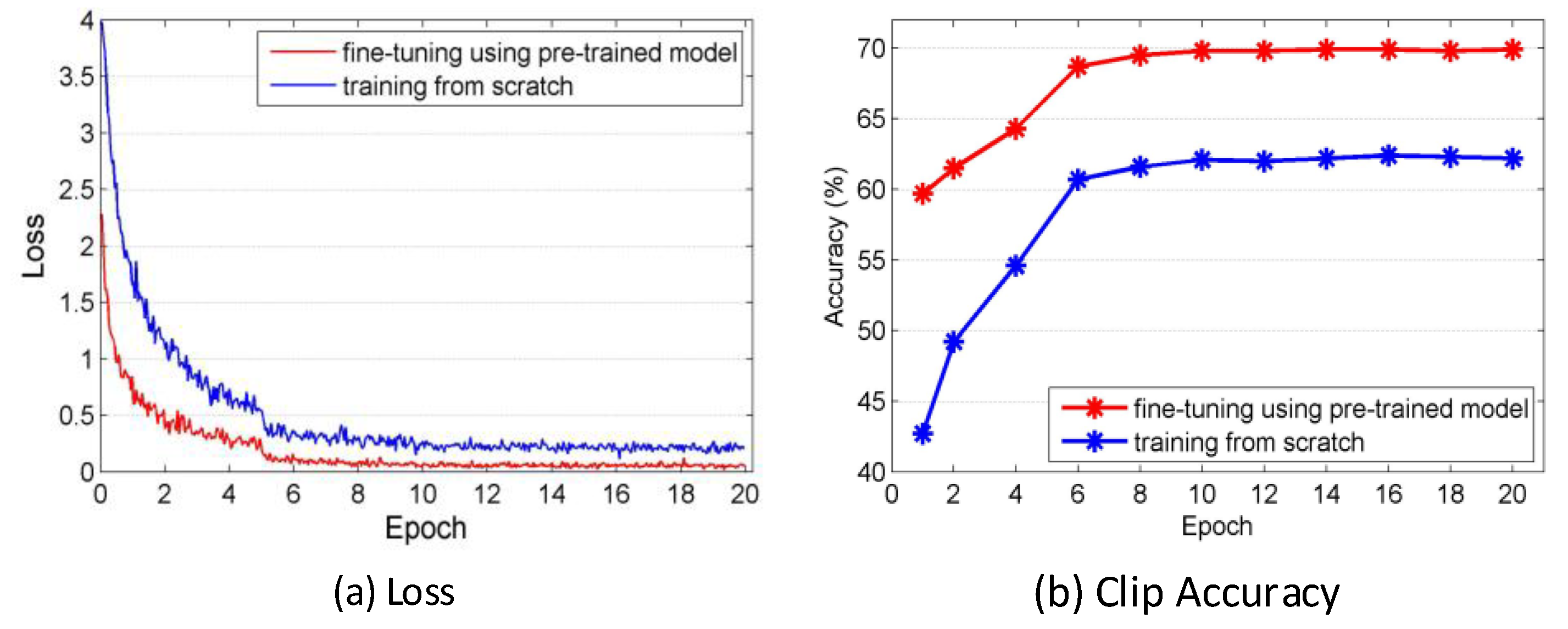
The pre-trained Res3D model provided by Tran et al. [13] takes 3-channel RGB clips as the input of CNN. To transfer the knowledge learned from the RGB to optical flow, we first design 3-channel optical flow. We extract the optical flow for each video action and discretize it by a linear transformation such that the optical flow values fall into the range [0, 255]. This transformation yields 2 channels of optical flow: the horizontal optical flow OF_x and the vertical optical flow OF_y. Then, we calculate the mean of OF_x and OF_y as the third channel. Figure 3 presents two consecutive frames, OF_x, OF_y and the 3-channel optical flow. This step ensures that the optical flow has same number of channels as the RGB used for the input of the Res3D architecture. To transfer the RGB knowledge to the optical flow, which is a new modality, we empirically increase learning rate, step size and the number of iteration during fine-tuning. Compared with RGB Res3D, we increase them in OF Res3D, respectively, by 10 times, 5 times and 5 times to accelerate the model updating. We conducted the evaluation of this fine-tuning and training from scratch in the OF stream of 8f temporal scale on UCF101 split-1. Figure 4 presents the comparison of these two methods by presenting training loss and clip accuracy. With the same number of iterations, the loss of the fine-tuning is smaller and the recognition accuracy using the model learned by fine-tuning is higher. As illustrated in Figure 4, after 20 epochs of iterations, the clip accuracy of OF Res3D learned by fine-tuning achieves 69.9%, while the clip accuracy of OF Res3D learned by training from scratch only achieves 62.2%. All these results show that this transfer learning works well and with the same number of iterations, fine-tuning using the pre-trained model outperforms the training from scratch.

3.3. Unsupervised Action Aton Mining

As basic action units, atoms capture the key spatiotemporal information in video sequences. In this paper, we mine atoms from the deep spatiotemporal information in each temporal scale. Obviously, atoms mining follows the same idea of video summarization, which compactly depicts the original video well using key elements, such as frames [36,37] or clips [38,39]. We propose to extend the maximization of mutual information (MMI) video summarization [40] to action atoms mining in the deep spatiotemporal space and model the temporal evolution of the mined atoms for action recognition.
Let Y be the set of spatiotemporal features for a video action A , Y = [ y 1 ,   y 2 , , y N ] , where y i n is the Pool5 feature extracted by Res3D, N is the clip number of action A and n = 512 is the dimension of the Pool5 feature. The summarization technology aims to use a subset Y * of size S to represent the original feature sets Y . In the MMI algorithm, the Y * that most reduces the entropy of the rest of the sets Y \ Y * is selected, which is formulated by
a r g m a x Y * I ( Y * ; Y \ Y * )  
This problem is resolved by a simple greedy algorithm that starts with Y * = and iteratively selects a feature y * from the remaining of the set Y \ Y * until the size of Y * is S . In each iteration, y * is selected to provide the maximum increase in mutual information. The objective function is formulated by
a r g m a x y * Y \ Y * ( H ( y * | Y * ) H ( y * | Y ¯ * ) )  
where Y ¯ * denotes Y \ ( Y * y * ) . H ( y * | Y * ) forces y * to be most different from the already selected Y * , while H ( y * | Y ¯ * ) forces y * to be most representative among the remaining features. Using the GP model [41], H ( y * | Y * ) is evaluated as a closed-form Gaussian conditional entropy:
H ( y * | Y * ) = 1 2 l o g ( 2 π e V ( y * | Y * ) )  
and V ( y * | Y * ) is evaluated as a closed-form conditional variance:
V ( y * | Y * ) = K ( y * , y * ) K T ( y * , Y * ) K 1 ( Y * , Y * ) K ( y * , Y * )  
where K is the covariance estimation. The objective function Equation (5) can be written in a closed form using Equations (3) and (4):
a r g m a x y * Y \ Y * K ( y * , y * ) K T ( y * , Y * ) K 1 ( Y * , Y * ) K ( y * , Y * ) K ( y * , y * ) K T ( y * , Y ¯ * ) K 1 ( Y ¯ * , Y ¯ * ) K ( y * , Y ¯ * )  
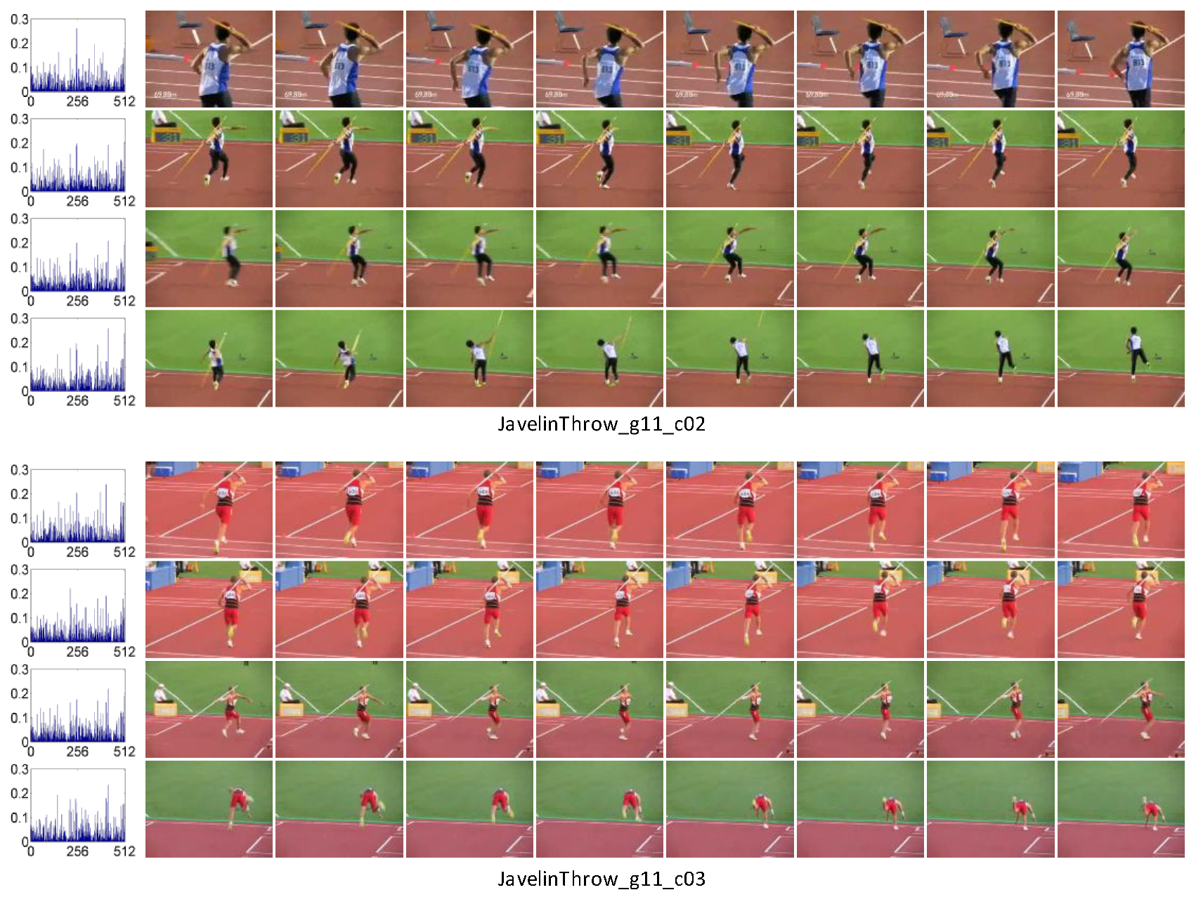
In each temporal scale of our method, to preserve considerably more of the key spatiotemporal information, we split the videos into 50% overlapped clips. We name the non-overlapped split clip in the original Res3D work “sparse clip” and name the overlapped split clip in this paper “dense clip.” For each video action, we use the trained Res3D to extract the Pool5 feature of the dense clips and use MMI summarization to mine the set of atoms with size S . For the video actions which have the dense clips less than S , the features of all the clips are considered as the atoms. Therefore, the maximum number of atoms associated with an action is S . Figure 5 illustrates the mined spatiotemporal atoms ( S = 4 ) sorted by timestamps and their corresponding clips in the RGB stream of 8f temporal scale. We also use the aforementioned metric video accuracy (Pool5) to measure the performance of unordered modeling on atoms ( S = 16 and S = 32 ) and compare it with random selection, sparse split and dense split in the RGB stream of 8f temporal scale. The results presented in Table 2 show that the performance of atoms mining is better than that of random selection and is close to that of the sparse split and dense split. However, atoms mining can be considered as a kind of simple ‘hard weight assignment,’ the features mined as atoms are ‘assigned’ to weight 1 and involved in the recognition. Thus, after atom mining, the number of features used to represent a video action is decreased, making it possible to train the LSTM with less memory and lower computational load. The temporal modeling of action atoms using LSTM is described in the next section.

3.4. Temporal Evolution Modeling on Atoms

An action is considered as a temporal evolution of the spatiotemporal atoms. Thus, unordered modeling is insufficient to represent and recognize an action. The RNN can be used to model the temporal evolution of the input sequences and has been applied to many sequence modeling tasks, including speech recognition [42], machine translation [43] and action recognition [44]. Therefore, we propose to employ LSTM, a RNN model, to model the temporal evolution of atoms for action recognition. Different from the CNN-RNN works [21,22,23,24] which applied an LSTM to the deep features of 2D CNN, we impose LSTM on the spatiotemporal atoms that are the key deep features of 3D CNN.
As a typical RNN architecture, LSTM has the capability to discover the action dynamics from extracted information by using memory cells to store and modify the internal state and has become increasingly popular. Figure 6 illustrates a LSTM cell at time step t . Given an input sequence X = ( x 1 , x 2 , ... , x t ) , the hidden state of the LSTM is formulated as follows:
i t = σ ( W i x x t + W i h h t 1 + b i )  
f t = σ ( W f x x t + W f h h t 1 + b f )  
o t = σ ( W o x x t + W o h h t 1 + b + o )  
g t = t a n h ( W g x x t + W g h h t 1 + b g )  
c t = f t c t 1 + i t g t  
h t = o t t a n h ( c t )  
where x t is the input at time step t , i t is the input gate, f t is the forget gate, o t is the output gate, c t is the memory cell state and h t is the hidden state. The input and forget gates determine whether to consider new information or forget old information. In addition, the output gate controls the amount of memory cell state that is passed to the hidden state to influence the computation in the next time step.
In each stream, we sort the atoms Y * by timestamps and denote the sorted atoms as X = { x 1 , x 2 , ... , x n u m } , where n u m m a x _ n u m , which are fed into LSTM to model the temporal evolution of action. We use a fully-connected layer on the top of the LSTM’S hidden state, followed by a softmax layer, to produce a prediction for each time step. As described in Section 3.3, the number of atoms ( n u m ) associated with each action is variable and the maximum number of atoms ( m a x _ n u m ) is S , therefore, we pad the atoms to reach the maximum number and perform dynamic LSTM. We tested three types of LSTM inferences: (a) the prediction at the m a x _ n u m time step, (b) the prediction at the n u m time step and (c) summing the predictions of the first n u m time steps. These three inferences are illustrated in Figure 7 and recognition results are presented in Table 3. The actual number of atoms is recorded by the n u m time step and for the videos with atoms less than m a x _ n u m , the input of the time steps from n u m + 1 to m a x _ n u m is padded with zero. Therefore, the prediction at the time steps from n u m + 1 to m a x _ n u m is not accuracy. While, the summing method considers the outputs of all the actual atoms and performs best, thus, it is used in our method.

3.5. Fusion Operations

Two fusion operations are used in our method. One is the RGB and OF streams fusion, the other is the multiple temporal scales fusion. First, we discuss the two streams fusion. As illustrated in Figure 8, after the deep spatiotemporal information is extracted from RGB and optical flow fields, there are three possible types of fusions.
  • Spatiotemporal information fusion (early fusion): The deep spatiotemporal information of the RGB and OF streams are fused. Then action atoms are mined from the fused spatiotemporal information.
  • Atom fusion (middle fusion): The action atoms mined from the deep spatiotemporal information of the RGB and OF streams are fused. Then the fused atoms are fed into LSTM.
  • Prediction fusion (late fusion): In each of the RGB and OF streams, LSTM are performed on the mined atoms. Then the softmax predictions of these two streams are fused.
For a video action, the information in the RGB and OF streams captures respective characteristic and in each stream, the clips of video action have different temporal dynamic. Therefore, the early fusion and middle fusion, in which the information of RGB and OF streams is fused and the temporal evolution of action in two steams is model using a same LSTM, would not perform as well as the late fusion. Moreover, in the middle fusion, the atoms of RGB and OF streams are mined in different feature spaces. Thus, the atoms in these two streams may correspond to different video clips and the middle fusion would perform worst among these three methods.
Early and middle fusions are feature-level fusions. We adopt summation, an effective feature-level fusion method for them. The late fusion is prediction-level fusion. We also use summation to fuse the softmax scores of the two streams. We compare the performance of single stream with two streams using different types of fusions in 8f temporal scale. The results are presented in Table 4. It is noticed that the recognition accuracy is improved from 87.9% to 92.2%, 91.5% and 92.4%, respectively, by the early, middle and late fusion, which demonstrates our design that the recognition performance benefits a lot from optical flow. On the other hand, the results also support our assumption that the late fusion outperforms the early and middle fusions and the middle fusion results in the worst performance, although the difference in accuracy among all three types of fusions is less than 1%.
For the multi-temporal-scale fusion, we sum the prediction of each temporal scale to form the final recognition result. We compare the recognition accuracy of the multi-temporal-scale method with single-temporal-scale methods. Table 5 reports the results, which show that the recognition accuracy can be significantly improved by fusing the prediction of the multiple temporal scales.

4. Evaluation

4.1. Datasets

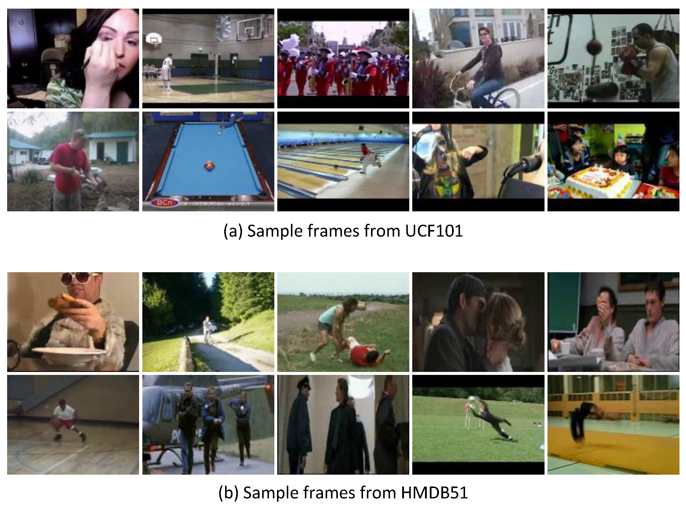
We evaluate the proposed approach on two action recognition datasets: UCF101 and HMDB5. Some sample frames are showed in Figure 9. These two datasets give large diversity in terms of actions and present the significant camera/background motion, cluttered background, variations of object appearance, pose, object scale, viewpoint and illumination conditions and so forth. Therefore, they are challenging for researches. On the other hand, these two datasets have gained popularity in recent years and most of state-of-the-art methods were evaluated on these two datasets. The UCF101 dataset contains 101 action classes and there are at least 100 videos for each class. The entire dataset contains 13,320 videos. And there are three training/testing splits in this dataset for evaluation. The HMDB51 dataset is a large collection of realistic videos from movies and web videos. The dataset is composed of 6766 videos from 51 action categories, with each category containing at least 100 videos. Similar to UCF101, HMDB51 also has three training/testing splits. Each action class has 70 videos for training and 30 videos for testing in each split.

4.2. Implementation Details

Optical Flow: We used the TVL1 algorithm [46] implemented in OpenCV with CUDA to extract optical flow and created the 3-channel optical flow described in Section 3.2.
Res3D Fine-tuning: To perform a fast fine-tuning, same with original Res3D work, we split the videos into sparse clips and took the sparse clips as the CNN input. We fine-tuned the 4f, 8f and 16f Res3D architectures using the pre-trained model. For each RGB Res3D architecture, the learning rate began at 0.001, decreased by 1/10 every epoch and stopped at 4 epochs. For each OF Res3D architecture, the learning rate started at 0.01, decreased by 1/10 every 5 epochs and stopped at 20 epochs. We used Momentum to optimize the network and set the momentum 0.9.
Atom Mining: By validation, we empirically mined 32 atoms in each stream for a video action.
LSTM Training: After validation, the number of memory cell and mini-batch in LSTM were set to 512 and 128, respectively. The learning rate and dropout were set to 0.005 and 0.7, respectively and the training stopped at 90 epochs. We selected softmax cross entropy loss and used SGD to optimize the network.

4.3. Performance Evaluation

In addition to the evaluation of the improvement by optical flow and multiple temporal scales in Section 3.5, in this section, we conducted extensive experiments to evaluate the improvements by atoms mining and temporal modeling. The experimental results are illustrated as a matrix in Table 6. The temporal modeling on the spatiotemporal feature of sparse clips was not evaluated because the m a x _ n u m of an action in the dynamic LSTM is 221, which requires so much memory that an ‘out of memory’ error occurred with our 4x GeForce GTX TITAN X GPU. Atoms mining reduces the m a x _ n u m to 32 and ensures that the dynamic LSTM consumes less memory and lower computational load, making the temporal modeling possible. The unordered modeling on atoms performs slightly worse than on sparse clips but the temporal modeling on the atoms resulted in the best performance in the evaluation matrix. The temporal modeling improves the performance of the atoms significantly. These results show that temporal modeling on the atoms is an effective method to represent and recognize actions.

4.4. Qualitative Run-Time Analysis

Compared with the unordered modeling in original Res3D work, our temporal method improves the recognition accuracy from 87.6% to 92.9% but due to the dense clip spits, two streams, multiple temporal scales and atoms mining involved, our method would spend much more time on recognition. In this section, we provide a qualitative run-time analysis of the proposed atoms temporal modeling method and compare it with unordered modeling method in the original Res3D work [13]. We only analyze the time consumption of the testing phase, which is a major focus in computer vision tasks. In our method, the testing phase contains optical flow extraction, feature extraction, atoms mining, temporal modeling and fusion. In the unordered modeling method, the testing phase contains optical flow extraction, feature extraction, clip merging and classification. For simplicity, we ignore the optical flow extraction which exists in both of our method and unordered method; we also ignore fusion in our temporal modeling and clip merging in unordered modeling, which take little time.
We present the measurement of each step in Table 7. All measurements were conducted on a computer with an Intel Core i7-5930K 3.5 GHz 12 CUP, GeForce GTX TITAN, 62 GB RAM and Ubuntu 14.04 LTS. In the atoms mining for a video, each iteration requires O ( N 4 ) to evaluate Equation (5), where N is the number of dense clips. We only present several measurements of atom mining for the videos with special number of dense clips.
With these measurements, it is easy to obtain the qualitative time consumption. Take a video action with 256 frames (about 8500 ms for 30 fps video) as an example, the time consumption of the recognition can be calculated as follows:
Unordered   modeling : 256 × 2.99 + 367.44 = 1132.88 ms
Our   method : 2 × 2 × 256 × ( 3.96 + 2.99 + 1.91 ) + 2 × ( 1197.43 + 282.62 + 0 ) + 2 × 3 × 0.46 = 12 , 035.5 ms
In Equation (13), the first and second ‘2’ denote the two streams and dense clips in feature extraction; the third and fourth ‘2’ denote the two streams in atoms mining and temporal modeling. 1197.43, 282.62 and ‘0’ denote 128 dense clips in 4f temporal scale, 64 dense clips in 8f temporal scale and 32 dense clips in 16f temporal scale, respectively. In this example, to recognize the action in an 8.5 s video with 30 fps, unordered modeling method spends 1.1 s and our temporal modeling method spends 12.04 s.
This run-time analysis shows that our temporal modeling method improves the recognition accuracy at the cost of run-time. For a real-life application, this limitation of our method should be considered. And the rough time consumption of the recognition can be calculated using the measurements in Table 7.

4.5. Comparison with State-of-the-Art Methods

We tested our proposed method on each training/testing split of both the UCF101 and HMDB51 datasets and reported the results according to the standard evaluation protocol, which is the mean video accuracy across the three splits. Table 8 presents the results of our method, state-of-the-art handcrafted methods and deep learning methods, including improved dense trajectories (iDT), SlowFusion, VGG16-style 3D convolution (C3D), ResNet18-style 3D convolution (Res3D), long term 3D convolution (LTC), two-stream model and others. In addition to the recognition accuracy, we also specify the network architecture and the fields of the CNN input. The results show that our method achieves recognition performance comparable to that of state-of-the-art methods.

4.6. Model Visualization

In CNN-based action recognition, it is difficult to explain the meaning of the extracted deep information using systemic and complete theory. However, visualization is an effective technique for gaining further insight into the trained CNN model and the extracted features. In addition to the visualization of the spatiotemporal atoms in Section 3.3, in this section, we visualize the convolution kernels and feature maps of Res3D and present the embedding visualization of the atoms.
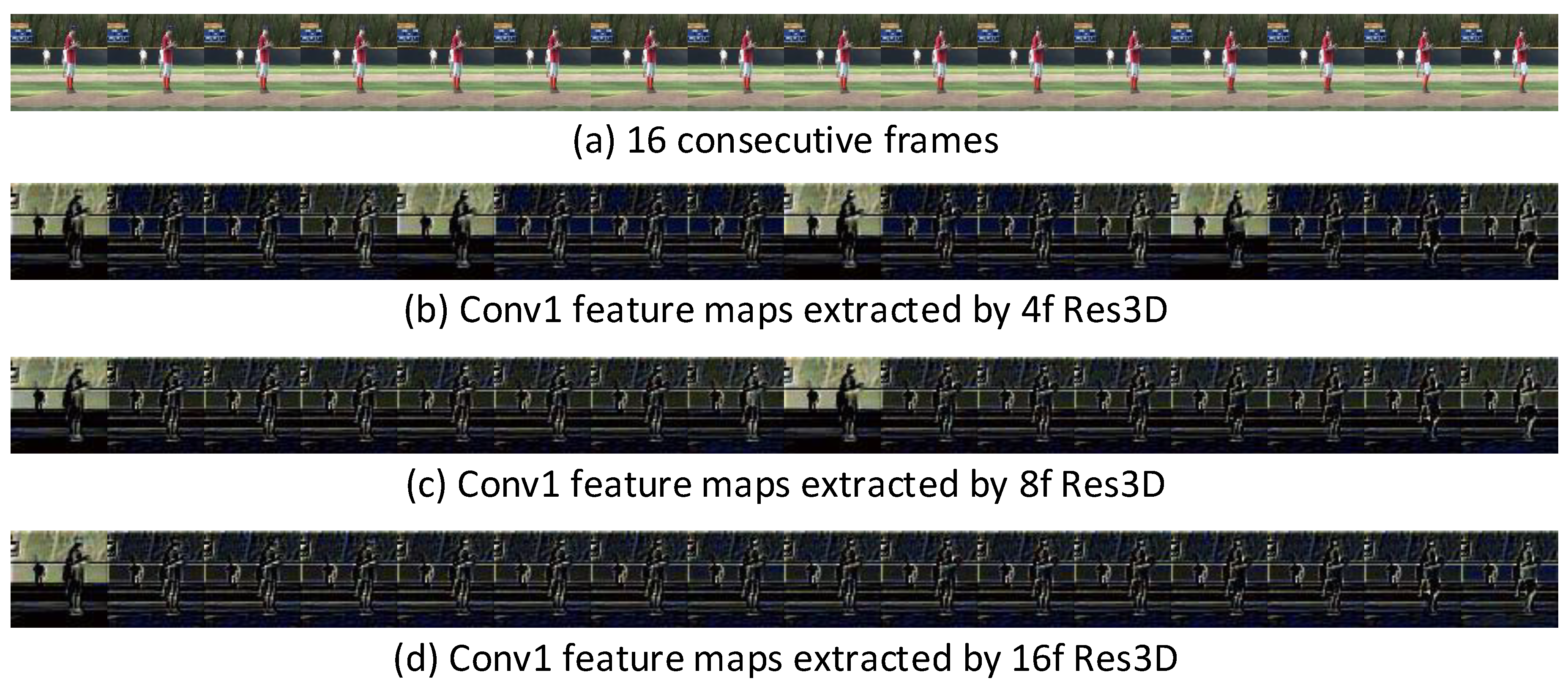
Figure 10 visualizes the extracted Conv1 feature maps of 16 consecutive frames (4, 2 and 1 clips for 4f, 8f and 16f Res3D, respectively). The figure shows that Res3D mainly captures the apparent (spatial) information from the first frame of the clip and captures the motion (temporal) information from the remaining 3, 7 and 15 frames of the clip. This observation confirms that different temporal scale information is extracted by the Res3D variants.
Figure 11 visualizes the learned conv1 kernel of the pre-trained Res3D, RGB 8f Res3D and OF 8f Res3D. Compared with RGB Res3D, OF Res3D is more different from the pre-trained Res3D. This result confirms that our settings speed up the process of kernel updating when the learned knowledge is transferred to a new modality.
The embedding visualizations of the mined atoms in RGB stream of the 4f, 8f and 16f temporal scales are illustrated in Figure 12. We average the atoms for each action and project them to 2D space using t-SNE [59]. The figure shows that the mined atoms all are semantically separable and can be used to represent video effectively.

5. Conclusions

An action can be naturally viewed as a temporal sequence of action atoms in different temporal scales. In this paper, we propose to model the temporal evolution of action atoms for action recognition. The action atoms are mined in the deep spatiotemporal space and the temporal modeling on atoms is demonstrated to be effective for representing the original video actions. Moreover, the atoms mining ensures that the dynamic LSTM consumes less memory and lower computational load, thus making the temporal modeling possible. The experimental results show that our proposed multi-temporal-scale spatiotemporal atoms modeling method achieves state-of-the-art recognition performance on two extremely challenging action recognition datasets: UCF101 and HMDB51.
In this study, we mine the spatiotemporal atoms in different temporal scales and model temporal evolution of atoms for each temporal scale. However, a realistic action is a single temporal sequence of the multi-temporal-scale atoms. Therefore, in our future work, we plan to study temporal modeling of hybrid multi-temporal-scale atoms. We could mine atoms simultaneously in different temporal scales and represent the video action using only one temporal evolution of the atoms. On the other hand, as analyzed in Section 4.4, our temporal method improves the recognition accuracy at the cost of run-time, therefore, the optimization of the run-time is a major work in the future.

Author Contributions

G.Y. conceived the idea of this paper and wrote this paper. G.Y. and X.L. performed the experiments and analyzed the experimental results. T.L. prepared the training samples. P.J. hosted the project of CNN-based action recognition and detection.

Funding

This research was funded by Youth Innovation Promotion Association, Chinese Academy of Sciences. Grant No. 2016336.

Conflicts of Interest

The authors declare no conflict of interest.

References

  1. LeCun, Y.; Bottou, L.; Bengio, Y.; Haffner, P. Gradient-based learning applied to document recognition. Proc. IEEE 1998, 86, 2278–2324. [Google Scholar] [CrossRef] [Green Version]
  2. Krizhevsky, A.; Sutskever, I.; Hinton, G. Imagenet classification with deep convolutional neural networks. In Proceedings of the Annual Conference on Neural Information Processing Systems, Lake Tahoe, NV, USA, 3–6 December 2012; pp. 1097–1105. [Google Scholar]
  3. Girshick, R.; Donahue, J.; Darrell, T.; Malik, J. Rich feature hierarchies for accurate object detection and semantic segmentation. In Proceedings of the IEEE Conference on Computer Vision and Pattern Recognition, Columbus, OH, USA, 23–28 June 2014; pp. 580–587. [Google Scholar]
  4. Farabet, C.; Couprie, C.; LeCun, Y. Learning hierarchical features for scene labeling. IEEE Trans. Pattern Anal. Mach. Intell. 2013, 35, 1915–1929. [Google Scholar] [CrossRef] [PubMed] [Green Version]
  5. Shelhamer, E.; Long, J.; Darrell, T. Fully convolutional networks for semantic segmentation. IEEE Trans. Pattern Anal. Mach. Intell. 2017, 39, 640–651. [Google Scholar] [CrossRef] [PubMed]
  6. Karpathy, A.; Toderici, G.; Shetty, S.; Leung, T.; Sukthankar, R.; Li, F. Large-scale video classification with convolutional neural networks. In Proceedings of the IEEE Conference on Computer Vision and Pattern Recognition, Columbus, OH, USA, 23–28 June 2014; pp. 1725–1732. [Google Scholar]
  7. Simonyan, K.; Zisserman, A. Two-stream convolutional networks for action recognition in videos. In Proceedings of the Advances in Neural Information Processing Systems, Montreal, QC, Canada, 8–13 December 2014; pp. 568–576. [Google Scholar]
  8. Yang, M.; Ji, S.; Xu, W.; Wang, J. Detecting human actions in surveillance videos. In Proceedings of the TREC Video Retrieval Evaluation Workshop, Fira, Greece, 8–10 July 2009. [Google Scholar]
  9. Ji, S.; Xu, W.; Yang, M.; Yu, K. 3D convolutional neural networks for human action recognition. In Proceedings of the International Conference on Machine Learning, Haifa, Israel, 21–24 June 2010; pp. 495–502. [Google Scholar]
  10. Baccouche, M.; Mamalet, F.; Wolf, C.; Carcia, C.; Baskurt, A. Sequential deep learning for human action recognition. In Proceedings of the International Conference on Human Behavior Unterstanding, Amsterdam, The Netherlands, 16 November 2011; pp. 29–39. [Google Scholar]
  11. Ji, S.; Xu, W.; Yang, M.; Yu, K. 3D convolutional neural networks for human action recognition. IEEE Trans. Pattern Anal. Mach. Intell. 2013, 35, 221–231. [Google Scholar] [CrossRef] [PubMed]
  12. Tran, D.; Bourdev, L.; Fergus, R.; Torresani, L.; Paluri, M. Learning spatiotemporal features with 3D convolutional networks. In Proceedings of the IEEE International Conference on Computer Vision, Venice, Italy, 22–29 October 2017; pp. 4489–4497. [Google Scholar]
  13. Tran, D.; Ray, J.; Shou, Z.; Changm, S.F.; Paluri, M. ConvNet architecture search for spatiotemporal feature learning. arXiv, 2017; arXiv:1708.05038. [Google Scholar]
  14. Feichtenhofer, C.; Pinz, A.; Zisserman, A. Convolutional two-Stream network fusion for video action recognition. In Proceedings of the IEEE Conference on Computer Vision and Pattern Recognition, Las Vegas, NV, USA, 26 June–1 July 2016; pp. 1933–1941. [Google Scholar]
  15. Zhang, B.; Wang, L.; Wang, Z.; Qiao, Y.; Wang, H. Real-time action recognition with enhanced motion vector CNNs. In Proceedings of the IEEE Conference on Computer Vision and Pattern Recognition, Las Vegas, NV, USA, 26 June–1 July 2016; pp. 2718–2726. [Google Scholar]
  16. Gao, Z.; Hua, G.; Zhang, D.; Jojic, N.; Wang, L. ER3: A unified framework for event retrieval, recognition and recounting. In Proceedings of the IEEE Conference on Computer Vision and Pattern Recognition, Honolulu, HI, USA, 21–26 July 2017. [Google Scholar]
  17. Yu, S.; Cheng, Y.; Su, S. Stratified pooling based deep convolutional neural networks for human action recognition. Multimedia Tools Appl. 2017, 76, 13367–13382. [Google Scholar] [CrossRef]
  18. Hochreiter, S.; Schmidhuber, J. Long short-term memory. Neural Comput. 1997, 9, 1735–1780. [Google Scholar] [CrossRef] [PubMed]
  19. He, K.; Zhang, X.; Ren, S.; Sun, J. Deep residual learning for image recognition. In Proceedings of the IEEE Conference on Computer Vision and Pattern Recognition, Las Vegas, NV, USA, 26 June–1 July 2016; pp. 770–778. [Google Scholar]
  20. Varol, G.; Laptev, I.; Schmid, C. Long-term temporal convolutions for action recognition. IEEE Trans. Pattern Anal. Mach. Intell. 2018, 40, 1510–1517. [Google Scholar] [CrossRef] [PubMed]
  21. Donahue, J.; Hendricks, L.; Guadarrama, L.; Rohrbach, M.; Venugopalan, S.; Darrell, T.; Saenko, K. Long-term recurrent convolutional networks for visual recognition and description. In Proceedings of the IEEE Conference on Computer Vision and Pattern Recognition, Boston, MA, USA, 7–12 June 2015; pp. 2625–2634. [Google Scholar]
  22. Donahue, J.; Hendricks, J.; Rohrbach, M.; Venugopalan, S.; Guadarrama, S.; Saenko, K.; Darrell, T. Long-term recurrent convolutional networks for visual recognition and description. IEEE Trans. Pattern Anal. Mach. Intell. 2017, 39, 677–691. [Google Scholar] [CrossRef] [PubMed]
  23. Ng, J.; Hausknecht, M.; Vijayanarasimhan, S.; Vinyals, O.; Monga, R.; Toderici, G. Beyond short snippets: Deep networks for video classification. In Proceedings of the IEEE Conference on Computer Vision and Pattern Recognition, Boston, MA, USA, 7–12 June 2015; pp. 4694–4702. [Google Scholar]
  24. Srivastava, N.; Mansimov, E.; Salakhutdinov, R. Unsupervised learning of video representations using LSTMs. In Proceedings of the International Conference on Machine Learning, Lille, France, 6–11 July 2015. [Google Scholar]
  25. Simonyan, K.; Zisserman, A. Very deep convolutional networks for large-scale image recognition. In Proceedings of the International Conference on Learning Representation, Banff, AB, Canada, 14–16 April 2014. [Google Scholar]
  26. Oliver, N.; Rosario, B.; Pentland, A. A bayesian computer vision system for modeling human interactions. IEEE Trans. Pattern Anal. Mach. Intell. 2000, 22, 255–272. [Google Scholar] [CrossRef]
  27. Wang, Y.; Mori, G. Hidden part models for human action recognition: Probabilistic versus max margin. IEEE Trans. Pattern Anal. Mach. Intell. 2011, 33, 1310–1323. [Google Scholar] [CrossRef] [PubMed]
  28. Laxton, B.; Lim, J.; Kriegman, D. Leveraging temporal, contextual and ordering constraints for recognizing complex activities in video. In Proceedings of the IEEE Conference on Computer Vision and Pattern Recognition, Minneapolis, MN, USA, 17–22 June 2007. [Google Scholar]
  29. Zeiler, M.; Fergus, R. Visualizing and understanding convolutional networks. In Proceedings of the European Conference on Computer Vision, Zurich, Switzerland, 6–12 September 2014; pp. 818–833. [Google Scholar]
  30. Chatfield, K.; Simonyan, K.; Vedaldi, A.; Zisserman, A. Return of the devil in the details: Delving deep into convolutional nets. In Proceedings of the British Machine Vision Conference, Nottingham, UK, 1–5 September 2014. [Google Scholar]
  31. Szegedy, C.; Liu, W.; Jia, Y.; Sermanet, P.; Reed, S.; Anguelov, D.; Erhan, D.; Vanhoucke, V.; Rabinovich, A. Going deeper with convolutions. In Proceedings of the IEEE Conference on Computer Vision and Pattern Recognition, Boston, MA, USA, 7–12 June 2015. [Google Scholar]
  32. Russakovsky, O.; Deng, J.; Su, H.; Krause, J.; Satheesh, S.; Ma, S.; Huang, Z.; Karpathy, A.; Khosla, A.; Bernstein, M.; et al. ImageNet large scale visual recognition challenge. Int. J. Comput. Vis. 2015, 115, 211–252. [Google Scholar] [CrossRef]
  33. Soomro, K.; Zamir, A.; Shah, M. UCF101: A Dataset of 101 Human Actions Classes from Videos in the Wild; Technical Report; University of Central Florida: Orlando, FL, USA, 2012. [Google Scholar]
  34. Kuehne, H.; Jhuang, H.; Garrote, E.; Poggio, T.; Serre, Y. HMDB: A large video database for human motion recognition. In Proceedings of the IEEE International Conference on Computer Vision, Barcelona, Spain, 6–13 November 2011. [Google Scholar]
  35. Wang, L.; Xiong, Y.; Wang, Z.; Qiao, Y. Towards good practices for very deep two-stream convnets. arXiv, 2015; arXiv:1507.02159. [Google Scholar]
  36. Liu, D.; Hua, G.; Chen, T. A hierarchical visual model for video object summarization. IEEE Trans. Pattern Anal. Mach. Intell. 2010, 32, 2178–2190. [Google Scholar] [CrossRef] [PubMed]
  37. Gong, B.; Chao, W.L.; Grauman, K.; Sha, F. Diverse sequential subset selection for supervised video summarization. In Proceedings of the Advances in Neural Information Processing Systems, Montreal, QC, Canada, 8–13 December 2014. [Google Scholar]
  38. Laganiere, R.; Bacco, R.; Hocevar, A.; Lambert, P.; Pais, G.; Ionescu, B.E. Video summarization from spatio-temporal features. In Proceedings of the ACM TRECVid Video Summarization Workshop, Vancouver, BC, Canada, 31 October 2008. [Google Scholar]
  39. Lu, Z.; Grauman, K. Story-driven summarization for egocentric video. In Proceedings of the IEEE Conference on Computer Vision and Pattern Recognition, Portland, OR, USA, 23–28 June 2013. [Google Scholar]
  40. Qiu, Q.; Jiang, Z.; Chellappa, R. Sparse Dictionary-based Attributes for Action Recognition and Summarization. arXiv, 2013; arXiv:1308.0290. [Google Scholar]
  41. Rasmussen, C.; Williams, C. Gaussian Processes for Machine Learning; The MIT Press: Cambridge, MA, USA, 2006. [Google Scholar]
  42. Graves, A.; Mohamed, A.; Hinton, G. Speech recognition with deep recurrent neural networks. In Proceedings of the International Conference on Acoustics, Speech and Signal Processing, Vancouver, BC, Canada, 26–31 March 2013; pp. 6645–6649. [Google Scholar]
  43. Sutskever, I.; Vinyals, O.; Le, Q.V. Sequence to sequence learning with neural networks. In Proceedings of the Advances in Neural Information Processing Systems, Montreal, QC, Canada, 8–13 December 2014; pp. 3104–3112. [Google Scholar]
  44. Baccouche, M.; Mamalet, F.; Wolf, C.; Garcia, C.; Baskurt, A. Action classification in soccer videos with long short-term memory recurrent neural networks. In Proceedings of the International Conference on Artificial Neural Networks, Thessaloniki, Greece, 15–18 September 2010; pp. 154–159. [Google Scholar]
  45. Olah, C. Understanding LSTM Networks. Available online: http://colah.github.io/posts/2015-08-Understanding-LSTMs/ (accessed on 17 Semptember 2018).
  46. Zach, C.; Pock, T.; Bischof, H. A duality based approach for realtime tv-L1 optical flow. In Proceedings of the DAGM Symposium on Pattern Recognition, Heidelberg, Germany, 12–14 September 2007; pp. 214–223. [Google Scholar]
  47. Wang, H.; Schmid, C. Action recognition with improved trajectories. In Proceedings of the IEEE International Conference on Computer Vision, Sydney, Australia, 1–8 December 2013; pp. 3551–3558. [Google Scholar]
  48. Peng, X.; Wang, L.; Wang, W.; Qiao, Y. Bag of visual words and fusion methods for action recognition. Comput. Vis. Image Underst. 2016, 150, 109–125. [Google Scholar] [CrossRef]
  49. Wang, L.; Qiao, Y.; Tang, X. Action recognition with trajectory-pooled deep-convolutional descriptors. In Proceedings of the IEEE Conference on Computer Vision and Pattern Recognition, Boston, MA, USA, 7–12 June 2015; pp. 4305–4314. [Google Scholar]
  50. Fernando, B.; Anderson, P.; Hutter, H.; Gould, S. Discriminative hierarchical rank pooling for activity recognition. In Proceedings of the IEEE Conference on Computer Vision and Pattern Recognition, Las Vegas, NV, USA, 26 June–1 July 2016; pp. 1924–1932. [Google Scholar]
  51. Kar, A.; Rai, N.; Sikka, K.; Sharma, G. AdaScan adaptive scan pooling in deep convolutional neural networks for human action recognition in Videos. In Proceedings of the IEEE Conference on Computer Vision and Pattern Recognition, Honolulu, HI, USA, 21–26 July 2017. [Google Scholar]
  52. Wang, X.; Farhadi, A.; Gupta, A. Actions transformations. In Proceedings of the IEEE Conference on Computer Vision and Pattern Recognition, Las Vegas, NV, USA, 26 June–1 July 2016; pp. 2658–2667. [Google Scholar]
  53. Zhao, S.; Liu, Y.; Han, Y.; Hong, R. Pooling the convolutional layers in deep ConvNets for video action recognition. IEEE Trans. Circuits Syst. Video Technol. 2017, 28, 1839–1849. [Google Scholar] [CrossRef]
  54. Park, E.; Han, X.; Berg, T.; Berg, A. Combining multiple sources of knowledge in deep CNNs for action recognition. In Proceedings of the IEEE Winter Conference on Applications of Computer Vision, Lake Placid, NY, USA, 7–9 March 2016; pp. 177–186. [Google Scholar]
  55. Li, Y.; Li, W.; Mahadevan, V.; Vasconcelos, N. VLAD3: Encoding dynamics of deep features for action recognition. In Proceedings of the IEEE Conference on Computer Vision and Pattern Recognition, Las Vegas, NV, USA, 26 June–1 July 2016; pp. 1951–1960. [Google Scholar]
  56. Qiu, Z.; Yao, T.; Mei, T. Learning spatio-temporal representation with pseudo-3D residual networks. In Proceedings of the IEEE International Conference on Computer Vision, Venice, Italy, 22–29 October 2017; pp. 5534–5542. [Google Scholar]
  57. Wu, Z.; Wang, X.; Jiang, Y.; Ye, H.; Xue, X. Modeling spatial-temporal clues in a hybrid deep learning framework for video classification. In Proceedings of the ACM Multimedia Conference, Seoul, Korea, 26–30 October 2018. [Google Scholar]
  58. Wu, Z.; Jiang, Y.; Ye, H.; Wang, X.; Xue, X.; Wang, J. Fusing Multi-Stream Deep Networks for Video Classification. arXiv, 2015; arXiv:509.06086. [Google Scholar]
  59. Maaten, D.; Hinton, G. Visualizing data using t-sne. J. Mach. Learn. Res. 2008, 9, 2579–2605. [Google Scholar]
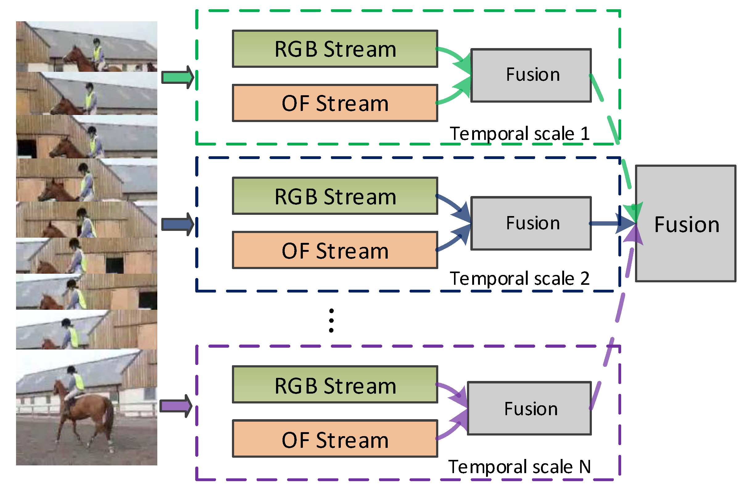
Figure 1. The framework of our proposed method.
Applsci 08 01835 g001
Figure 2. The illustration of a stream in our proposed method.
Applsci 08 01835 g002
Figure 3. Two consecutive frames, optical flow in the horizontal and vertical directions and 3-channel optical flow.
Applsci 08 01835 g003
Figure 4. Comparison of two types of training: (a) fine-tuning using the pre-trained model; and (b) training from scratch. The experiment is conducted in in the optical flow (OF) stream of 8f temporal scale on UCF101 split-1.
Applsci 08 01835 g004
Figure 5. The mined atoms (S = 4) sorted by timestamps and their corresponding clips in the 8f temporal scale.
Applsci 08 01835 g005
Figure 6. The structure of long short-term memory (LSTM) unit [45].
Applsci 08 01835 g006
Figure 7. Three types of LSTM inferences.
Applsci 08 01835 g007
Figure 8. Fusions of the RGB and OF streams.
Applsci 08 01835 g008
Figure 9. Sample frames from UCF101 and HMDB51.
Applsci 08 01835 g009
Figure 10. Visualization of the Conv1 feature maps. Res3D captures the appearance information in the first frame of the clip and thereafter captures the motion information.
Applsci 08 01835 g010
Figure 11. Visualization of the kernels. The shape of the 64 Conv1 kernels is 3 × 3 × 7 × 7 (C*T*H*W). The visualization shows the learned Conv1 kernels with T = 2, which are arranged in 8 × 8 with a 4× upscale.
Applsci 08 01835 g011
Figure 12. Atoms embedding visualizations of the 4f, 8f and 16f temporal scales on UCF101 training split-1. The averaged atom of each action is visualized as a point and the averaged atoms that belong to the same action class have the same color.
Applsci 08 01835 g012
Table 1. Res3D architectures and the recognition results on UCF101 split-1.
LayersBuilding BlocksShape of the Input
Res3D-8
(8f Res3D)
Res3D-4DRes3D-4B3
(4f Res3D)
Res3D-4B4Res3D-16DRes3D-16SRes3D-16B2
(16f Res3D)
Conv13 × 7 × 7, 643 × 8
× 112 × 112
3 × 4
× 112 × 112
3 × 4
× 112 × 112
3 × 4
× 112 × 112
3 × 16
× 112 × 112
3 × 8
× 112 × 112
3 × 16
× 112 × 112
Conv2_x [ 3 × 3 × 3 , 64 3 × 3 × 3 , 64 ] × 2 64 × 8
× 56 × 56
64 × 4
× 56 × 56
64 × 4
× 56 × 56
64 × 4
× 56 × 56
64 × 16
× 56 × 56
64 × 8
× 56 × 56
64 × 16
× 56 × 56
Conv3_x [ 3 × 3 × 3 , 128 3 × 3 × 3 , 128 ] × 2 64 × 8
× 56 × 56
64 × 4
× 56 × 56
64 × 4
× 56 × 56
64 × 4
× 56 × 56
64 × 16
× 56 × 56
64 × 8
× 56 × 56
64 × 8
× 56 × 56
Conv4_x [ 3 × 3 × 3 , 256 3 × 3 × 3 , 256 ] × 2 128 × 4
× 28 × 28
128 × 2
× 28 × 28
128 × 4
× 28 × 28
128 × 2
× 28 × 28
128 × 8
× 28 × 28
128 × 4
× 28 × 28
128 × 4
× 28 × 28
Conv5_x [ 3 × 3 × 3 , 512 3 × 3 × 3 , 512 ] × 2 256 × 2
× 14 × 14
256 × 1
× 14 × 14
256 × 2
× 14 × 14
256 × 2
× 14 × 14
256 × 4
× 14 × 14
256 × 2
× 14 × 14
256 × 2
× 14 × 14
FCInnerProduct
Softmax
512 × 1
× 7 × 7
512 × 1
× 7 × 7
512 × 1
× 7 × 7
512 × 1
× 7 × 7
512 × 2
× 7 × 7
512 × 1
× 7 × 7
512 × 1
× 7 × 7
Clip Accuracy--82.5%75.2%80.4%79.1%No Functional84.4%84.5%
Video Accuracy
(Res5b)
--87.6%81.3%85.9%84.6%No Functional88.3%88.7%
Video Accuracy
(Pool5)
--87.1%81.1%85.3%84.2%No Functional87.8%88.1%
Table 2. Comparison of the atoms mining with other methods in the RGB stream of 8f temporal scale on UCF101 split-1.
Features SelectionVideo Accuracy (Pool5)
Sparse split87.1%
Dense split87.3%
16/32 atoms mining86.7%/86.9%
16/32 random selection86.3%/86.4%
Table 3. Comparison of different LSTM inferences in the RGB stream of 8f temporal scale on UCF101 split-1.
MethodsVideo Accuracy
the max_num step20.4%
the num step87.2%
Summation of the first num steps87.9%
Table 4. Comparison of single stream with two streams in the 8f temporal scale on UCF101 split-1.
MethodsVideo Accuracy
Single Stream
RGB stream87.9%
OF stream84.7%
Two Streams
Early fusion92.2%
Middle fusion91.5%
Late fusion92.4%
Table 5. Comparison of multi-temporal-scale method with single-temporal-scale methods on UCF101 split-1.
MethodsVideo Accuracy
Single-temporal-scale
4f temporal scale92.1%
8f temporal scale92.4%
16f temporal scale92.2%
Multi-temporal-scale
Our method92.9%
Table 6. The results matrix of the performance evaluation experiment in the RGB stream of 8f temporal scale on UCF101 split-1.
Sparse ClipsAtoms
Unordered Modeling87.1%86.9%
Temporal Modeling--87.9
Table 7. Time consumption measurement of each step in the unordered modeling and temporal modeling.
Unordered ModelingOur Temporal Modeling
Feature extraction:
8f Res3D: 2.99 ms/frame
Feature extraction:
4f Res3D: 3.96 ms/frame
8f Res3D: 2.99 ms/frame
16f Res3D: 1.91 ms/frame
Classification:
25088-dimensional feature: 367.44 ms
Atoms Mining:
0–32 clips: 0 ms (No need atom mining)
33 clips: 101.21 ms
64 clips: 282.62 ms
96 clips: 836.72 ms
128 clips: 1197.43 ms
Temporal modeling (with classification): 0.46 ms
Table 8. Comparison of our method with state-of-the-art methods.
MethodsUCF101HMDB51CNN ArchitectureInput of CNN
Handcrafted Representation Methods
iDT [47]85.9%57.2%----
iDT+HSV [48]87.9%61.1%----
Deep Learning Methods (2D CNN)
SlowFusion [6]65.4%--AlexNetRGB
TDD [49]90.3%63.2%ZFNetRGB + OF
Two-stream
(Averaging/SVM) [7]
86.9%/
88.0%
58.0%/
59.4%
CNN-MRGB + OF
Improved Two-stream [14]92.5%65.4%VGG-16RGB + OF
RankPooling [50]91.9%65.4%VGG-16RGB + OF
AdaScan [51]89.4%54.9%VGG-16RGB + OF
Transformation [52]92.4%62.0%VGG-16RGB + OF
Trajectory Pooling [53]92.1%65.6%VGG-16,CNN-MRGB + OF
Multi-Source [54]89.1%54.9%VGG-19RGB + OF
ConvPooling [23]88.2%--GoogLeNetRGB + OF
SlowFusion [6]65.4%--AlexNetRGB
Deep Learning Methods (3D CNN)
C3D [12]85.2%--C3DRGB
VLAD3 [55]90.5%--C3DRGB
LTC [20]91.7%64.8%LTCRGB + OF
Res3D [13]85.8%54.9%Res3DRGB
P3D-ResNet [56]88.6%--P3D-ResNetRGB
C3D [12]85.2%--C3DRGB
Deep Learning Methods (2D CNN-RNN)
LRCN [22]82.3%--ZFNetRGB + OF
LSTM [23]88.6%--GoogLeNetRGB + OF
Hybrid Deep [57]91.3%--VGG-19,CNN-MRGB + OF
Unsupervised [24]84.3% VGG-16RGB + OF
Multi-stream [58]92.6% VGG-19,CNN-MRGB + OF
LRCN [22]82.3%--ZFNetRGB + OF
Deep Learning Methods (3D CNN-RNN)
Our method92.9%66.7%Res3DRGB + OF