Recent Progress in Fast Distributed Brillouin Optical Fiber Sensing

Abstract

Brillouin-based optical fiber sensing has been regarded as a good distributed measurement tool for the modern large geometrical structure and the industrial facilities because it can demodulate the distributed environment information (e.g., temperature and strain) along the sensing fiber. Brillouin optical time domain analysis (BOTDA), which is an excellent and attractive scheme, has been widely developed thanks to its high performance in a signal-to-noise ratio, a spatial resolution, and sensing distance. However, the sampling rate of the classical BOTDA is severely limited by several factors (especially the serially frequency-sweeping process) so that it cannot be suitable for the quickly distributed measurement. In this work, we summarize some promising breakthroughs about the fast BOTDA, which can be named as an optical frequency comb technique, an optical frequency-agile technique, a slope-assisted technique, and an optical chirp chain technique.

1. Introduction

By combining the laser and optical fiber, optical fiber sensing technology has been developed rapidly, which is widely used in the fields of civil structure health monitoring, modern industrial controlling, and national defense security. Compared with the traditional resistance and capacitance-based electronic sensors, optical fiber sensing has clear advantages [1]: optical fiber is not only the low-loss optical transmission medium but also the continuously deployed sensors. The optical fiber is easy to access to the all-optical network in adverse working conditions thanks to its lightweight and compact structure while maintaining high resolution, high sensitivity, and a wide measurement range. Then, physical parameters outside of the fiber can also be obtained by measuring the acoustic impedance along the fiber, which has been demonstrated in recent reports [2,3]. Because of the above merits, a variety of optical fiber sensors are developed for modern industry. Among them, the distributed ultra-fast BOTDA, which has more practical application value is urgently needed.

From the 1990s, the Brillouin-based optical fiber sensing [4,5,6,7] has drawn much interest since it can offer an attractive solution to the societal concern for distributed dynamic measurement. Two optical waves are launched into the fiber under test (FUT) in the opposite direction. When their frequency-detuning is close to the Brillouin frequency shift (BFS) of the FUT, the power will be dramatically transferred from the high-frequency optical wave to the low-frequency optical wave via the stimulated Brillouin scattering (SBS) effect [8,9]. By scanning the frequency-detuning, the distributed Brillouin gain spectrum (BGS) can be obtained and its central frequency (i.e., BFS) computed by curve-fitting has a linear relationship [1,4,5,10,11] with an environmental strain or temperature.

Up to now, there are several Brillouin-based sensing schemes, which are shown in

Table 1. Several Brillouin-based optical fiber sensing schemes.

	Time-Domain	Frequency-Domain	Correlation-Domain
Reflectometer	Brillouin optical time domain reflectometer (BOTDR) [18,19]	Brillouin optical frequency domain reflectometry (BOFDR) [20]	Brillouin optical correlation domain reflectometry (BOCDR) [6,21]
Analysis	Brillouin optical time domain analysis (BOTDA) [22,23]	Brillouin optical frequency domain analysis (BOFDA) [24,25]	Brillouin optical correlation domain analysis (BOCDA) [6,26]

. For one end schemes, Brillouin reflectometers are achieved by only injecting an optical pump wave into the FUT and detecting the backscattering Brillouin signal to demodulate the spontaneous BGS. To enhance the Brillouin signal, two end schemes (i.e., analysis method) are obtained by injecting a counter-propagating probe wave resulting in an enhanced SBS effect. Considering the interaction domains for the optical waves, three subcategories can be classified as the time-domain, the frequency-domain, and the correlation domain. For the time-domain approach, a high signal-to-noise ratio (SNR), a long sensing distance [12], and a high sampling rate can be provided but the spatial resolution is restricted in ~1 m [13]. For the frequency-domain approach, high sensitivity and a wide dynamic range can be obtained but the sampling rate is limited. As for the correlation-domain approach, a high spatial resolution can be achieved but it is suitable for points sensing with a high sampling rate. In addition, some schemes based on the Brillouin dynamic grating [10,14,15,16,17] is also restricted in the static measurement.

In this paper, we mainly focus on the BOTDA scheme. By analyzing the limiting factors of the measurement speed for classical BOTDA scheme, several improved BOTDA schemes proposed in recent years are summarized for distributed dynamic measurements.

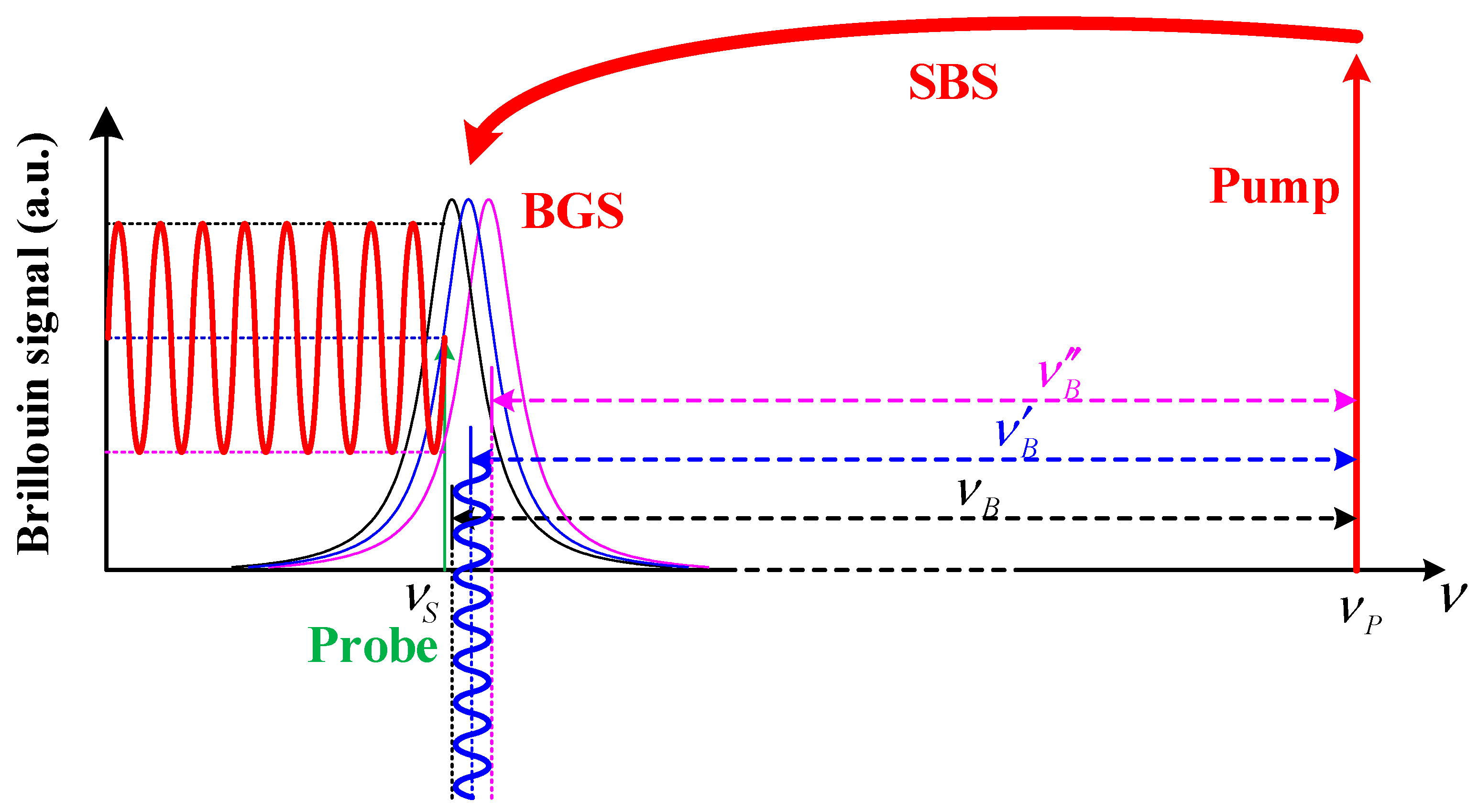
2. Operation Principle

When a high power optical wave propagates along an ordinary standard single-mode fibers (SMF), a moving density grating (i.e., the acoustic wave) will be excited in the core of the SMF via an electrostriction effect through SBS effect, which will induce a Doppler shift (i.e., the BFS) for its backscattered Stokes wave and the BFS is given by References [8,9,27].

$${\nu }_B=\frac{{\mathsf{\Omega }}_B}{2\pi }\equiv \frac{2n_{\mathrm{eff}}{V}_A}{{\lambda }_p}$$

(1)

where $n_{\mathrm{eff}}$ is the effective core refractive index, $V_A$ is the acoustic velocity, and ${\lambda }_p$ is the wavelength of the pump wave in a vacuum. Generally, for a silica SMF, the BFS is ~11 GHz [1,5,9] at the communication wavelength of 1550 nm. It is noted that the BFS has a good linear relationship [1,11] with the strain and temperature of the fiber and is given by the equation below.

$${\nu }_B={\mathrm{C}}_B^{\epsilon }\Delta \epsilon +{\mathrm{C}}_B^T\Delta T+{\nu }_{B0}$$

(2)

where ${\nu }_{B0}$ is the initial BFS of the fiber, ${\mathrm{C}}_B^{\epsilon }$ and ${\mathrm{C}}_B^T$ are the strain and temperature coefficients of the BFS, respectively, and $\Delta \epsilon$ and $\Delta T$ are the variations of strain and temperature. Based on Equation (2), the distributed variations of the strain or temperature are demodulated by measuring the distributed BFS.

To measure the distributed BFS, the typical BOTDA scheme is operated by the “Pump-Probe” method [5,11,28,29], which is shown in Figure 1. A pulsed-pump is injected into the FUT at the position z = 0 while a CW-probe wave is injected into the FUT at the position z = L, which is shown in Figure 1a. For a probe wave with different frequencies, their amplitudes will be amplified by obeying the BGS curve while their phases will be modulated obeying the Brillouin phase-shifted spectrum (BPSS), which is illustrated in Figure 1b. If the frequency of the pump pulse maintains constant, the distributed BGS will be constructed through segment-by-segment scanning of the frequency of the probe wave. A well-defined position distribution along the FUT corresponding to a round-trip time of the pump pulse can be achieved by identifying the start and end points of the amplified Brillouin signal. The spatial resolution is defined as $c\tau /\left(2n_{\mathrm{eff}}\right)$, which corresponds to the pump pulse’s width $\tau$. Then, the distributed BGS can be obtained through a frequency-sweeping process for the probe wave and is curve-fitted to get the distributed BFS.

Based on the Maxwell equations representing the optical waves and the Navier-Stokes equation describing the acoustic variation in the FUT [30,31], the BOTDA scheme can be depicted by the formula below.

$$\begin{array}{c}\frac{\partial E_P}{\partial z}+\frac{n}{c}\frac{\partial E_P}{\partial t}=i{g}_o\rho E_S-\frac{\alpha }{2}{E}_P\\ -\frac{\partial E_S}{\partial z}+\frac{n}{c}\frac{\partial E_S}{\partial t}=i{g}_o{\rho }^{*}{E}_L-\frac{\alpha }{2}{E}_S\\ \frac{\partial \rho }{\partial t}+\mathsf{\Gamma }\rho =i{g}_a{E}_P{E}_S^{*}\end{array}$$

(3)

where $E_P\mathrm{and}{E}_S$ are the electric fields of the optical pump and probe fields, respectively. $\rho$ is the material density along the FUT. $*$ is the complex conjugate operator. $i$ is the imaginary symbol. $g_o\mathrm{and}{\mathrm{g}}_a$ are the coupling coefficients of the optical wave and the acoustic wave, respectively. $\mathrm{\Gamma }={\mathrm{\Gamma }}_B/2+i\left({\mathsf{\Omega }}_{\mathrm{B}}-\mathsf{\Omega }\right)=1/{\tau }_{\mathrm{P}}$ where ${\tau }_p$ is the phonon lifetime.

For the probe wave, it experiences not only the Brillouin amplification but the Brillouin phase-shift [11] (i.e., the vector SBS effect), which is shown in Figure 1b. The BGS and BPSS can be depicted by the equations below.

$$g_{SBS}({\nu }_S,z)=g_p\frac{\Delta {\nu }_B^2}{4\Delta {\nu }^2+\Delta {\nu }_B^2}\otimes P_P({\nu }_P,z)$$

(4)

$${\phi }_{SBS}({\nu }_S,z)=g_p\frac{2\Delta {\nu }_B\Delta \nu }{4\Delta {\nu }^2+\Delta {\nu }_B^2}\otimes P_P({\nu }_P,z)$$

(5)

where $g_p$ is the gain factor at the line center, $\Delta {\nu }_B$ is the Brillouin linewidth, $\Delta \nu =\Delta {\nu }_P-\left(\Delta {\nu }_S+\Delta {\nu }_B\right)$ is the frequency detuning of the probe wave from the BFS, $P_P({\nu }_P,z)$ is the power spectrum of the pump wave, and the sign ⊗ represents the convolution operator.

3. The Speed Limitations of the Distributed Measurement for the Classical BOTDA Scheme

For the classical BOTDA scheme, the temperature or strain measurement time is usually several seconds to several minutes long, which limits its applications to a static or a slowly-varying measurement. Based on References [32,33,34], the expression of the maximum sampling rate can be modified to become the equation below.

$$f_{s\_\mathrm{BOTDA}}=\frac{1}{\left(T_{round\_trip}\cdot N_{code}\cdot N_{a\nu e}+T_{switch}\right)\cdot N_f}$$

(6)

where $T_{round\_trip}=2nL/c$ is the round-trip time of the pump pulse, which is an inherent limitation related to the length of the sensing fiber and L. $N_{code}$ is the code length of the pump pulse number. For instance, this value should be set to 2 for the differential double-pulse (DPP) BOTDA scheme [32] while it depends on the encoding bits and rules for the coding approach [33]. $N_{a\nu e}$ is the times of the averaging. $T_{switch}$ is the frequency-switching time of the microwave generator (MWG). $N_f$ is the effective frequency-sweeping number for the probe wave, which is used to measure the whole BGS and restricts the dynamic range. For the classical BOTDA, generally, $N_{code}=1$, $N_{a\nu e}$ is several tens for a polarization maintaining fiber (PMF) and thousands for a standard SMF, the $T_{switch}$ is on the order of ~ms scale that is limited by the property of the MWG, and $N_f$ is usually ~100 for a frequency interval of several MHz to obtain a wide dynamic range of several hundreds of MHz.

To increase the sampling rate of the BOTDA scheme, the recent hotspots researched are focused on reducing the $T_{switch}$ by using the high-performance electrical devices, decreasing the $N_f$ by using novel sensing curves instead of BGS, and BPSS and de-multiplexing $N_f$ in a frequency-domain and a time-domain.

4. Developments of the Fast BOTDA Schemes

Recently, to improve the performance of the BOTDA scheme, several novel fast schemes are proposed: optical frequency comb (OFC) technique, optical frequency-agile (OFA) technique, slope-assisted (SA) technique, and the optical chirp chain (OCC) technique.

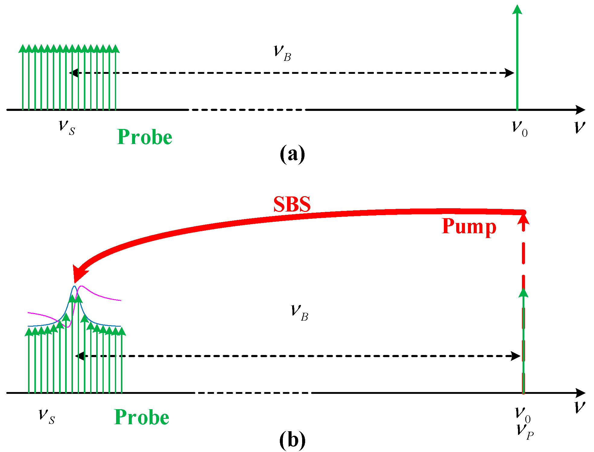
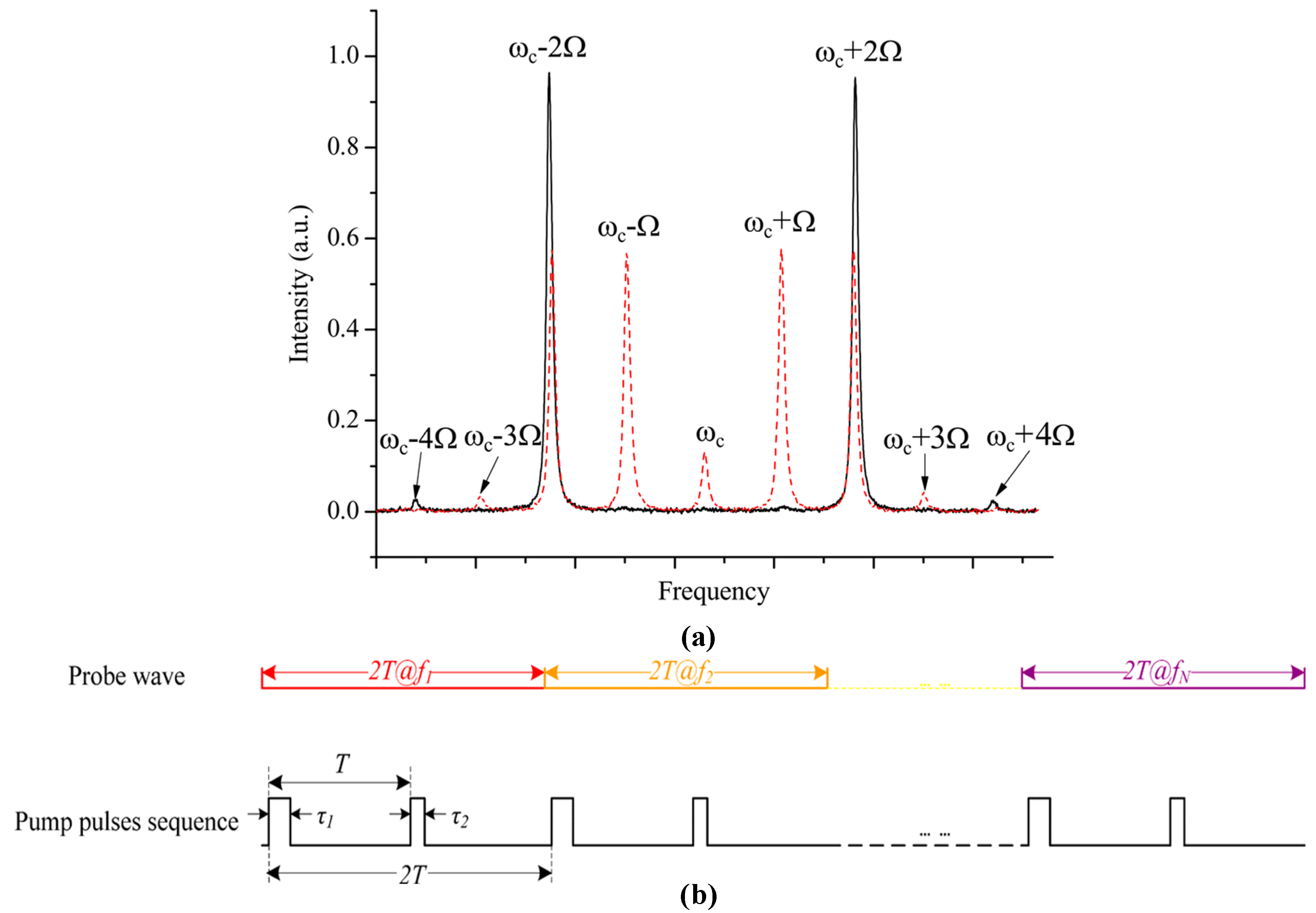
4.1. Optical Frequency Comb Based Fast BOTDA

To avoid the point-by-point frequency-sweeping process, an OFC wave, which has already been used in precise metrology [35], is employed to quickly acquire the whole BGS in the frequency-domain. As shown in Figure 2a, generally the probe wave with the frequency ${\nu }_0$ is single-sideband modulated into an optical carrier and an OFC sideband while an optical pulse is used as a pump wave whose central frequency is equal to the optical carrier, which is shown in Figure 2b. The beating Brillouin signal can be amplified by just injecting a pump pulse when the frequency span of the OFC covers and the BFS of the FUT in a frequency-domain via the SBS amplification. Then, the distributed BGS can be demodulated using a fast Fourier transform (FFT) of the beating Brillouin signal.

To improve the performance of the OFC-based BOTDA, a dual-polarization OFC-probe wave [36] is generated based on the orthogonal frequency-division multiplexing (OFDM) modulation. Both of the upper sideband OFC in the x-polarization axis and the lower sideband OFC in the y-polarization axis are injected into a 1.08 km standard SMF with a counter-propagating pump pulse, which results in a Brillouin loss (in Figure 3a) and a Brillouin gain (in Figure 3b), respectively. The distributed BGS (in Figure 3c) can be reconstructed by calculating the absolute spectra of the Brillouin loss and the Brillouin gain. Then, the combined Brillouin signal can be drastically enhanced by coherent detection and polarization combination. Without frequency-sweeping, polarization noise and averaging a temperature measurement along a 1.08 km SSMF is through the interaction of the OFDM-probe and just one pump pulse. It can be clearly concluded that the maximum sampling rate of this scheme is only confined by the fiber length. Then, the temperature change can be clearly recognized with a spatial resolution of 20.48 m and the comparison of the BGSs at a different position is displayed in Figure 3d.

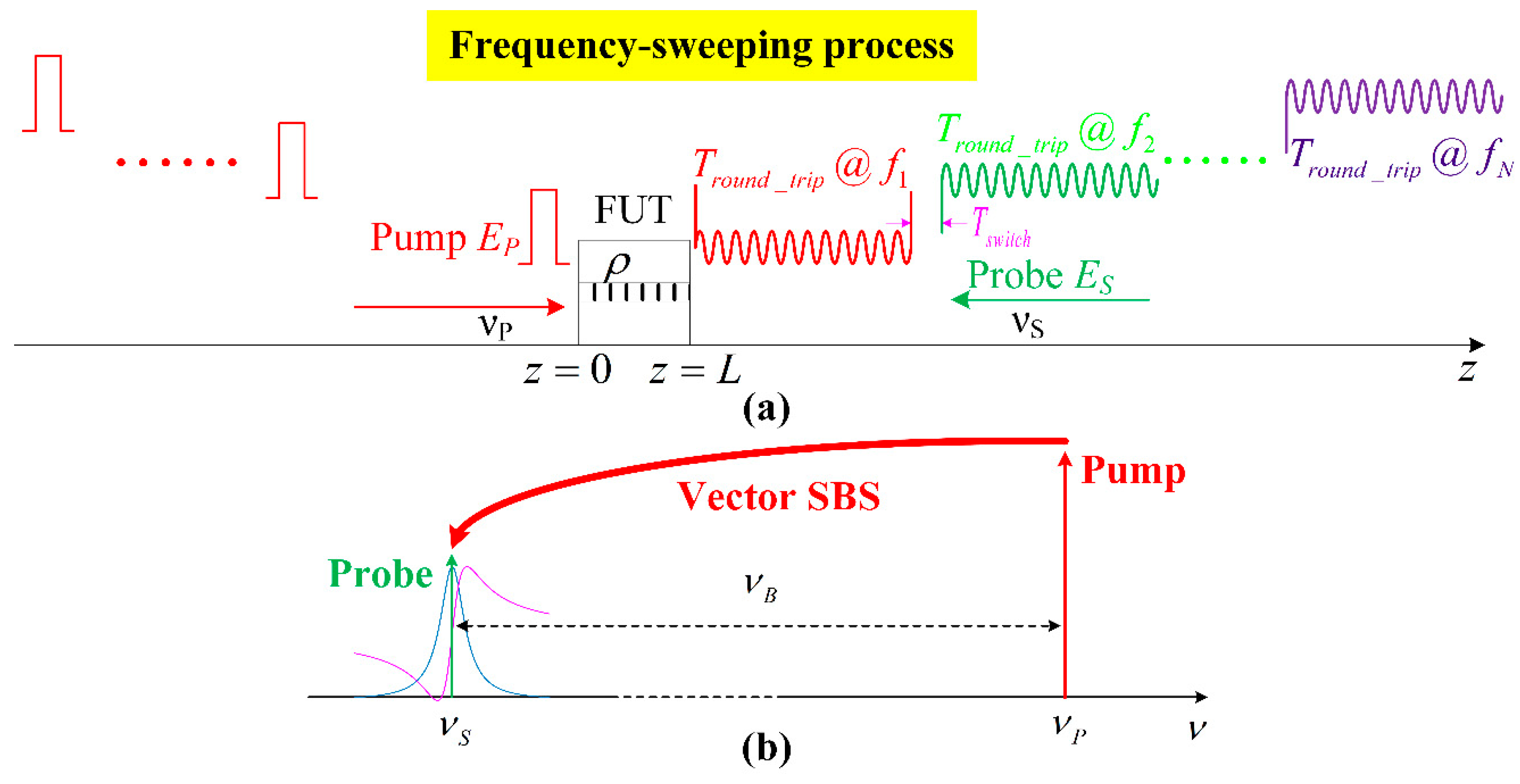
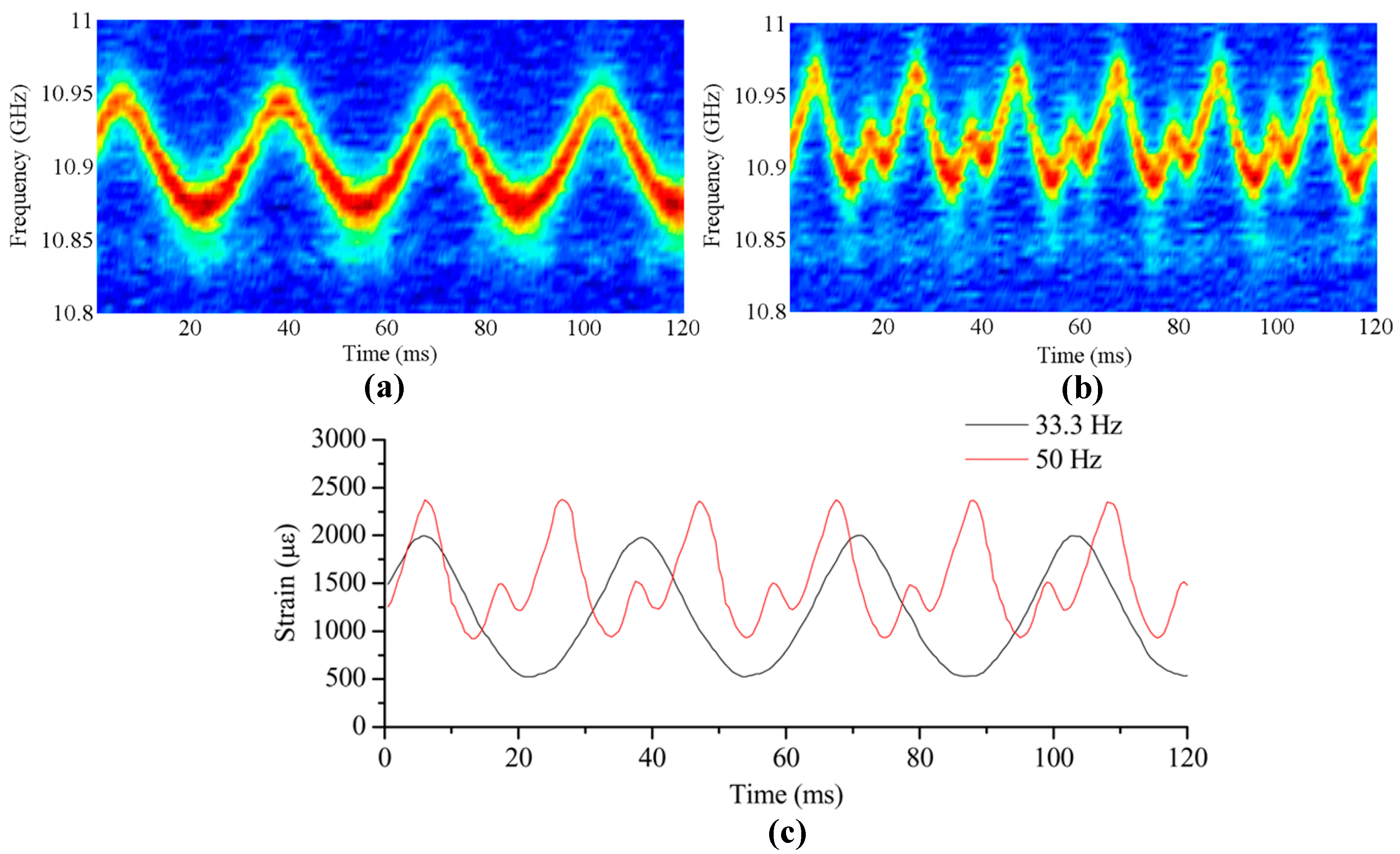
4.2. Optical Frequency-Agile Based Fast BOTDA

As the development of electrical devices, an OFA-based fast BOTDA [34] is proposed to compress the frequency-sweeping process in the time-domain. As shown in Figure 4, for example, an optical wave in the left path is intensity-modulated into a series of pulses with a fixed central frequency used as the pump pulse while an optical wave in the right path is frequency-modulated into the OFA-probe wave by employing an arbitrary waveform generator (AWG) whose output waveform can be user-defined. After the user-defined microwave for the frequency-sweeping process is tailored into the microwave segments with equal duration beyond the round-trip time $T_{round\_trip}$ and equal frequency interval, all waveforms of the microwave segments are recorded into the memory of the AWG on a head-to-end link mode in a time-domain so that the $T_{switch}$ is dropped to ~ns. Ultimately, the continuous probe wave is single-sideband modulated by the output user-defined microwave (i.e., frequency-agile microwave) generating the OFA-probe wave. Each probe wave segment can be amplified by the corresponding pump pulse and its amplitude obeys the BGS curve. Based on Equation (6), the sampling rate of this scheme can be effectively increased because the frequency-switching time $T_{switch}$ can be neglected. However, the bandwidth of the AWG is required to be around ~11 GHz corresponding to the BFS of the FUT, which has increased the cost of the system.

To cut down the bandwidth requirement for the AWG and to increase the spatial resolution, a combination scheme of the second-order sideband modulation (SOSM) [32] and DPP technique [23,28,30,32,37] is proposed, which is shown in Figure 5. By appropriately selecting the maximum working point of an intensity modulator, the even-order optical sidebands are excited by loading the frequency-agile microwave while the optical carrier and odd-order sidebands are perfectly suppressed (see the black line in Figure 5a). Subsequently, the lower second order optical sideband is selected as the probe wave by an optical filter so that the frequency requirement of the frequency-agile microwave output from the AWG can be decreased to around 5.5 GHz [32]. At the same time, two optical pulses with a narrow width difference are encoded as a pump pulse pair (i.e., $N_{code}=2$), which is the black line in Figure 5b. This results in two high SNR Brillouin signals. Then, a reconstructed Brillouin signal with a high SNR can be obtained by subtracting the two Brillouin signals. Its spatial resolution is also equal to the subtraction of the spatial resolutions for these two Brillouin signals. However, the sampling rate of this scheme is also cut by half because it needs two times the duration for the OFA-probe wave to avoid the overlap of the two Brillouin signals.

In the experiment, a dynamic strain measurement with a 20-cm spatial resolution [32] is obtained by subtracting two Brillouin signals generated by two pump pulses of 52 ns and 50 ns, respectively. Then, two time-evolutions of the BGSs at the end of the 50-m FUT, corresponding to two different mechanical vibrations, are measured with a 2-kHz sampling rate, as shown in Figure 6a,b. The vibration waveforms are calculated by curve-fitting the BGSs, which is shown in Figure 6c.

To further decrease the bandwidth requirement for AWG, a dual-modulation scheme [38] is proposed by employing a single-frequency modulation for a pump wave and an OFA modulation for the probe wave, which is shown in Figure 7a. The optical carrier of the right branch is first modulated by a sinusoidal microwave with a fixed frequency of ~10 GHz output from a microwave source. Subsequently, the first order sideband is selected to be intensity-modulated into a 10-ns pulse by an optical filter, which is used as an up-converted pump pulse. For the left branch, a single-sideband modulator is driven by the frequency-agile microwave output from the AWG to generate a down-converted OFA-probe wave. As a result, a lower bandwidth requirement of only several hundred of MHz for the AWG is achieved as the frequency difference between the pump pulse and the OFA-probe wave, which can cover the BFS of the FUT. A damped oscillation with the central frequency of 12.3 Hz is measured by a sampling rate of 100 Hz (see Figure 7b).

4.3. Slope-Assisted Fast BOTDA

Different from the classical BOTDA that needs curve-fitting of the whole BGS to get the sensing curve, an SA-BOTDA [39,40] is implemented by selecting one of the two slopes of the BGS as the sensing curve. As shown in Figure 8, the central part of the left slope of the BGS can be simply regarded as a linear section. After fixing the probe wave’s frequency in the middle of this linear section (i.e., $N_f=1$), the intensity of the Brillouin signal will be changed as the whole BGS as well as the BFS, which is shifted by the environmental strain or temperature. After injecting the one-shot pump pulse (i.e., $N_{code}=1$), the distributed BFS along the fiber can be easily demodulated by substituting the intensity of the Brillouin signal into the expression of the pre-fitted linear section. It should be noted that, based on Equation (6) and without averaging, the maximum sampling rate is also confined by the fiber length L. However, the frequency variation of the SA-BOTDA is limited within 30-MHz corresponding to the linewidth of the BGS. To increase the dynamic range, recent researchers are concentrating on increasing the slope number and enlarging the available dynamic range of the single monotonous slope of the sensing curve.

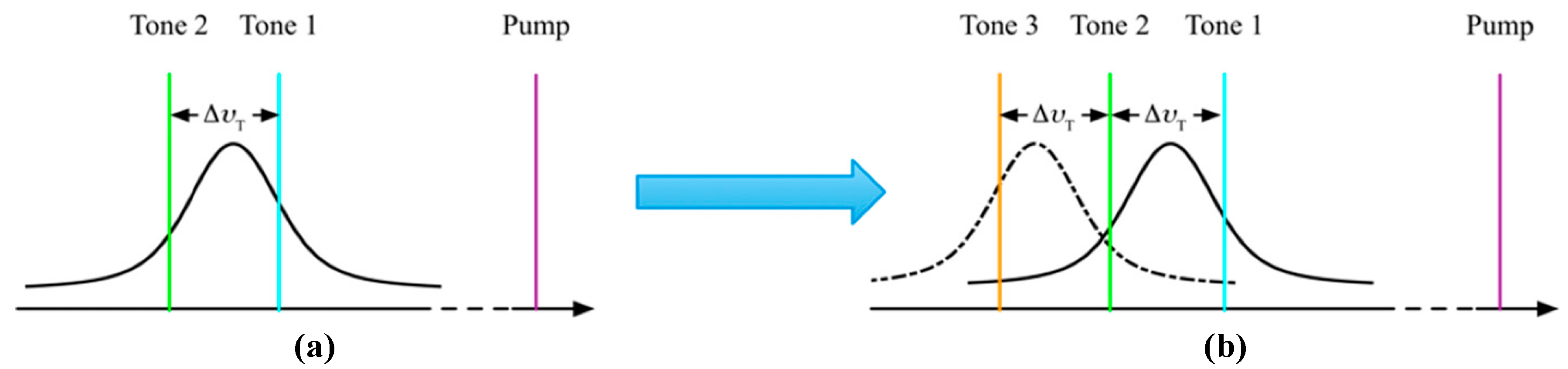
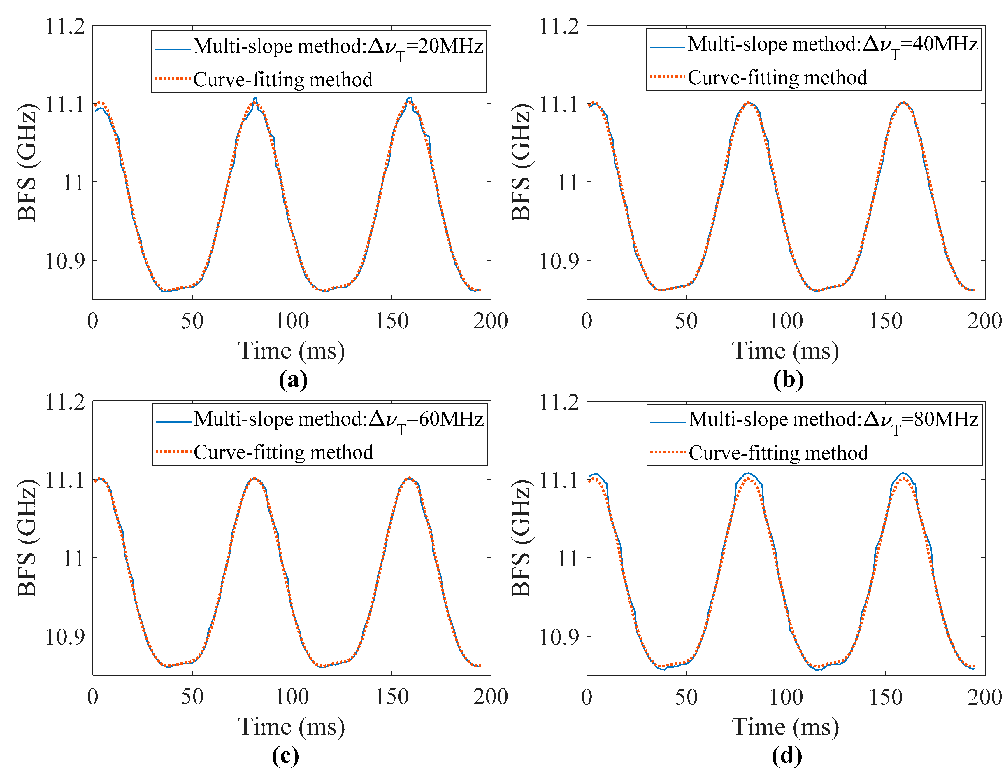
4.3.1. Increasing the Slope Numbers

To make full use of both slopes of the BGS, a coefficient $R_B$ [41] is defined as the ratio of the two Brillouin gains corresponding to the two tones (i.e., $N_f=2$), which is shown in Figure 9a. It should be noted that the profile of $R_B$ has a wide monotonous slope and its insensitivity of the power fluctuation for the pump pulse. The BFS of the FUT can be demodulated based on the value of $R_B$. Furthermore, a multi-slope-assisted BOTDA is implemented using the OFA-probe wave, which is shown in Figure 9b. A special OFA-probe wave, which has a large frequency interval, is generated and amplified by obeying the BGS profile from which two neighbor and the maximum Brillouin signals are chosen to calculate the value of $R_B$ and the BFS. In this scheme, a wide dynamic range is obtained by adding the tones at the expense of the sampling rate.

In the experiment, a dynamic strain with a vibration frequency of ~12.8 Hz is acquired and demodulated at the sampling rate of 1 kHz. The maximum strain variation of 5000 με corresponding to the BFS change of 241 MHz is realized with the frequency intervals ranging from 20 MHz to 80 MHz (see Figure 10a–d). It should be noted that the maximum sampling rate in theory of this scheme can reach 10 times higher than that of the typical OFA-based BOTDA thanks to its large frequency interval.

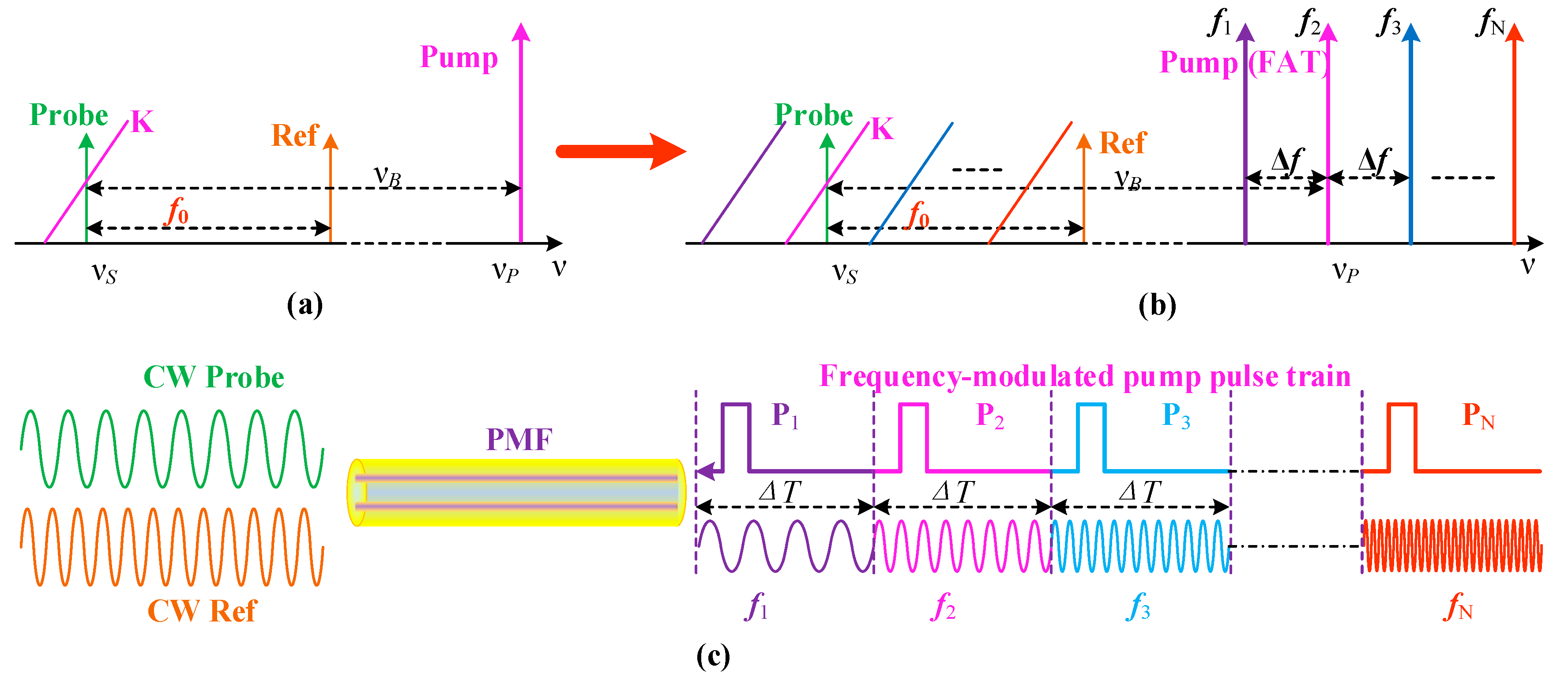
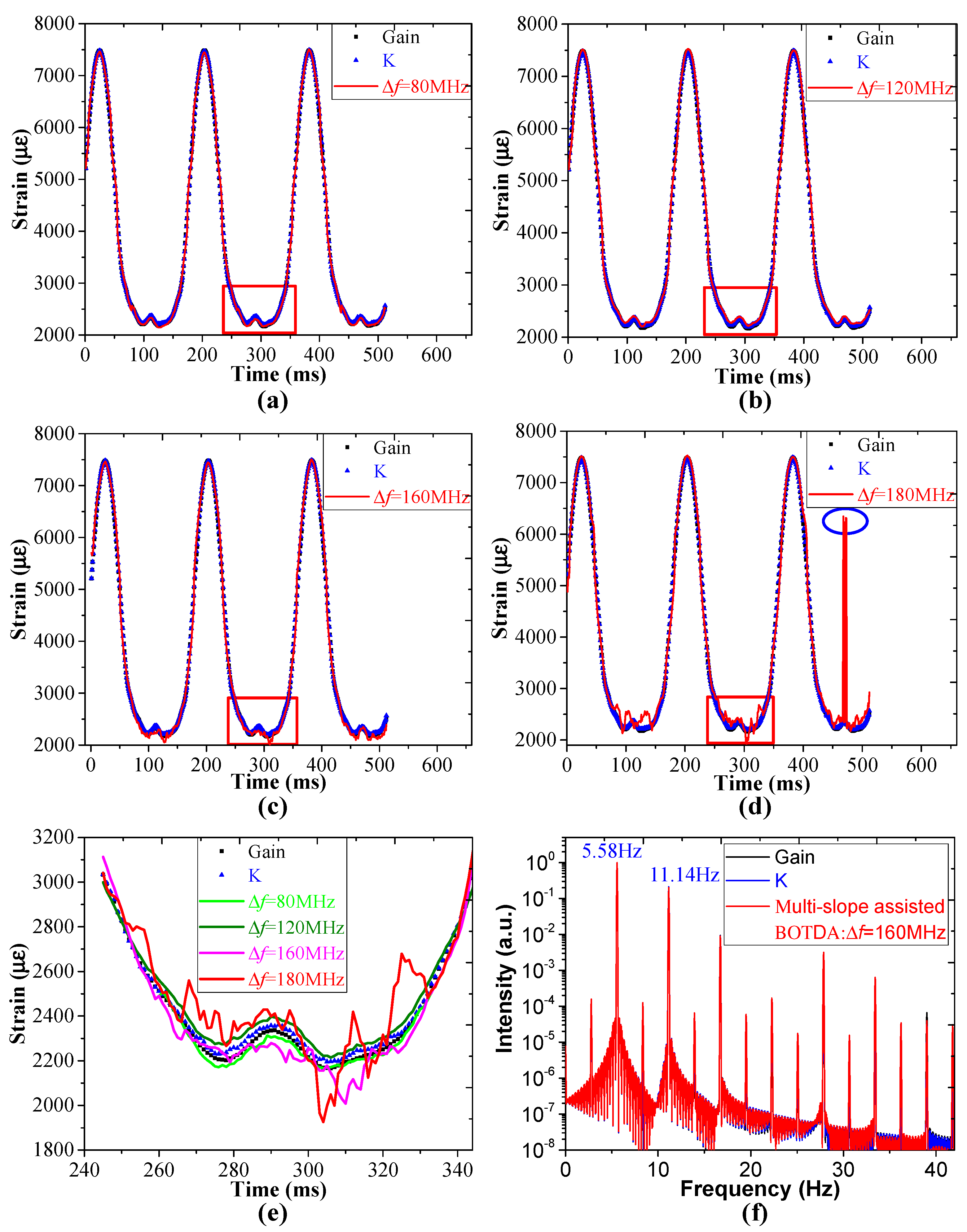
4.3.2. Enlarging the Monotonous Slope of the Sensing Curve

Instead of the slope of the BGS, the slopes of the BPSS [43,44] and RF phase-shift profile [45] are selected as the sensing curve resulting in the dynamic ranges of 40 MHz and 128 MHz, respectively. Recently, a dimensionless coefficient K [11] is defined as the expression below.

$$K({\nu }_S,z)=\frac{{\phi }_{SBS}({\nu }_S,z)}{g_{SBS}({\nu }_S,z)}$$

(7)

where the coefficient K spectrum (KS) is a function of the frequency detuning $\Delta \nu$. The KS is insensitive to the power fluctuation of the pump pulse so as to improve the SNR. Especially for the situation of a continuous pump wave, Equation (7) can be simplified as the formula below.

$$K({\nu }_S,z)=\frac{2\Delta \nu }{\Delta {\nu }_B}$$

(8)

where the KS is a straight line with the slope value of $2/\left(\Delta {\nu }_B\right)$.

The measured spectra of the BGS, the BPSS, and the KS are obtained as shown in Figure 11 for a pump pulse of 20 ns. By Lorentzian-fitting (blue line) the BGS, its BFS and linewidth are computed to be 10.694 GHz and 48 MHz, respectively. The available frequency range of the slopes of the BGS and BPSS for dynamic sensing is narrower than the linewidth of the BGS while that of the monotonous slope of the KS is beyond 200 MHz, which is wider than fourfold of the linewidth of the BGS. Moreover, the SNR of the KS is better than that of the BGS and the BPSS.

A single-slope-assisted BOTDA scheme is proposed using KS as the sensing curve, which is shown in Figure 12a. The probe wave and a reference wave (Ref) are injected into the sensing fiber while the pump pulse is injected in the opposite direction. The beating Brillouin signal between the probe wave and the Ref wave can be detected via the heterodyne detection and demodulated based on the IQ demodulation algorithm [46], which results in the BGS value and the BPSS value. Then, the K value can be calculated based on Equation (7). Generally, working at the K = 0 point, the dynamic BFS is computed by substituting the K value into the expression of the KS sensing curve. Then, to further enlarge the dynamic range, a multi-slope-assisted BOTDA scheme is also assembled through the combination of the KS and the OFA techniques, which is shown in Figure 12b,c. In our scheme, the pump pulses are frequency-modulated using the OFA technique so that each pump pulse corresponds to one K value. Subsequently, the K value closest to zero is selected and substituted into the expression of the KS sensing curve to calculate the BFS of the FUT.

The results of dynamic strain measurements using the multi-slope-assisted BOTDA are shown in Figure 13, which are demodulated based on two methods i.e., the traditional curve-fitting method and the hybrid KS + OFA method, respectively. The reference time traces are demodulated through curve-fitting the BGS and the KS to calculate the BFS with a frequency number of $N_f=101$ and a frequency interval of 4 MHz. As shown in Figure 13a–d, the time traces (red line) are demodulated by searching the minimum |K| to compute the BFS for the frequency interval of 80 MHz, 120 MHz, 160 MHz, and 180 MHz, and for the frequency number $N_f$ of 6, 4, 3, and 3, respectively. It can be clearly seen that the time traces are in good agreement with the reference time trace in Figure 13a–c while several distortion points (the blue ellipse in Figure 13d) and severe waveform distortion (zoom-in view in Figure 13e) are generated for the frequency interval of 180 MHz. Therefore, the maximum frequency interval for this scheme is 160 MHz, which is twice of that of the BGS-based multi-slope-assisted BOTDA scheme [42]. This results in a doubled sampling rate. The dynamic strain with a maximum variation of about 5372.9 με (254.3 MHz) and a 5.58 Hz main vibration frequency is obtained at the sampling rate of 1 kHz, as illustrated in Figure 13f.

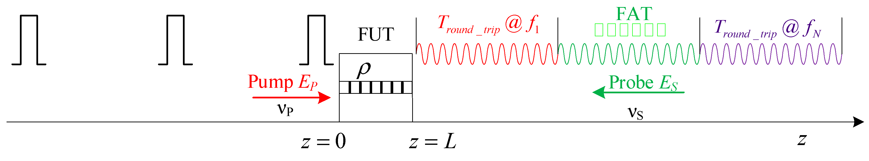
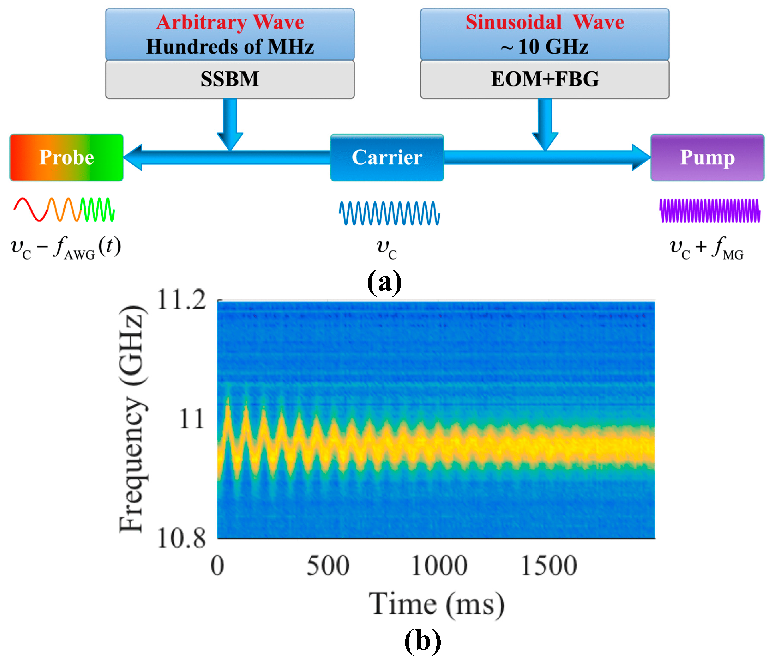
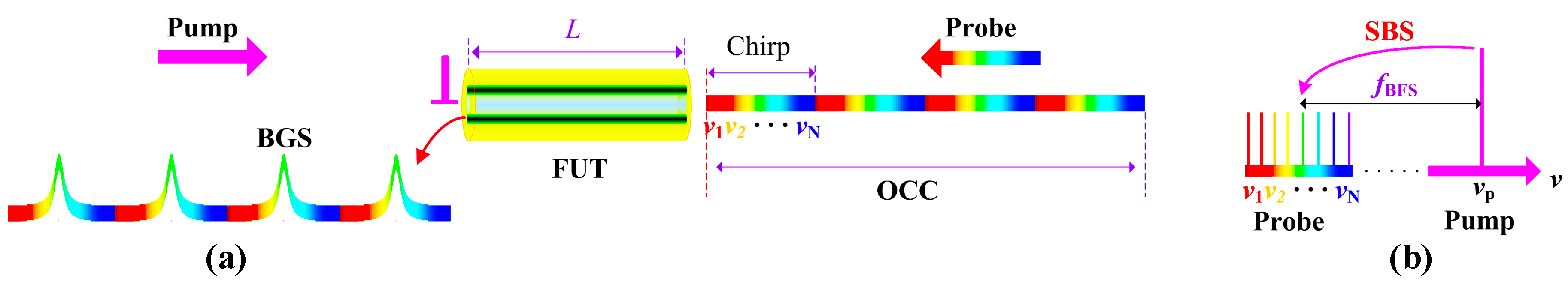
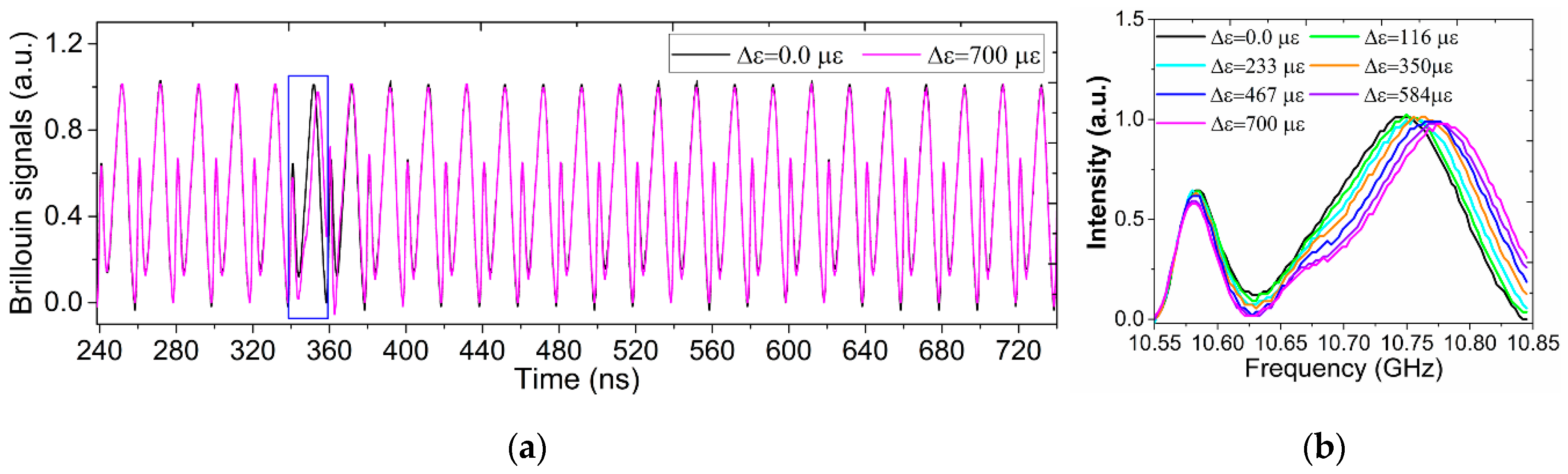
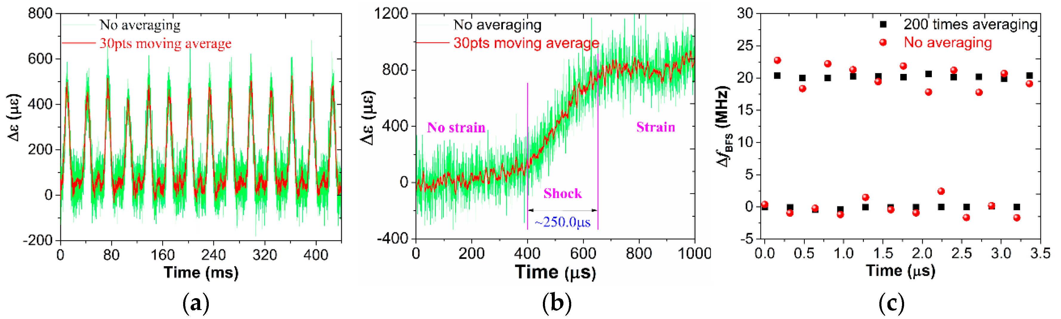
4.4. Optical Chirp Chain Technique for Fast BOTDA

Different from recovering the BGS in frequency-domain for the OFC-based BOTDA, OCC-based BOTDA schemes [1,47] have been implemented to recover the whole BGS or BLS in the time-domain thanks to the time-frequency mapping of the chirp signal. As demonstrated in Figure 14a, with a high-performance AWG, the frequency-sweeping process can be compressed into an optical chirp segment with a few tens of nanoseconds and the frequency ranged from ${\nu }_1$ to ${\nu }_N$ by the OFA technique. The chirp distribution of this optical chirp segment is given by the equation below.

$$f_{AWG}\left(t\right)=f_1+\eta ·t$$

(9)

where $f_1$ is the initial frequency and $\eta$ is the frequency chirp value.

Subsequently, the OCC-probe wave is formed by head-to-tail linking several segments in the time domain. The duration of the OCC-probe wave should be longer than the round-trip time of the pump pulse. When single-shot pump pulse interacts with every optical chirp segment and the frequency span of the OCC-probe wave covers the BFS of the FUT (see Figure 14b), the BGS can be revealed at every segment in the time domain. The parameters of the OCC-BOTDA scheme can be summarized as $T_{switch}<<T_{round\_trip}$, $N_{code}=1$ and $N_f=1$. Based on Equation (6), the maximum sampling rate of the OCC-based BOTDA without averaging is only limited by the fiber length.

The distributed BGS of a static strain measurement is demonstrated in Figure 15a. The BGS is excited every 20 ns [1]. A zoom-in view within the blue box is illustrated in Figure 15b, which clearly shows that the main peaks have frequency-shifts as the strain ranges from 0.0 με to 700 με.

Lastly, the OCC-based BOTDA scheme is examined by three different types of vibration: a periodic mechanical vibration, a mechanical shock, and a switch event. The vibrational waveforms (see Figure 16a–c) are measured at the sampling rates of 25 kHz, 2.5 MHz, and 6.25 MHz, respectively.

5. Challenges and Future Perspectives

A comparison between the traditional frequency-sweeping method and the above four improved schemes is shown in

Table 2. Comparison of the proposed BOTDA schemes in this work.

	Averaging Time ${\mathit{N}}_{\mathit{ave}}$	Frequency-Switching Time ${\mathit{T}}_{\mathit{switch}}$	Effective Frequency-Sweeping Number ${\mathit{N}}_{\mathit{f}}$
Frequency-sweeping	~100	~ms	~100
OFC + OFDM	≥1	0	1
OFA	~100	~ns	~100
SA + OFA	≥1	~ns	≥1
OCC	≥1	~ns	1

. Since the length L of the FUT is the inherent limitation and the code length $N_{code}$ have the same influence on these schemes, the two factors haven’t been listed in Table 2. For the averaging time $N_{a\nu e}$, the OFC + OFDM scheme can eliminate the polarization noise while the OCC scheme can enhance it through a cross-correlation algorithm [1,48,49]. Since all the frequency segments are injected into FUT at the same time for the OFC + OFDM scheme, its frequency-switching time is ideally zero. Compared to the ~ms frequency-switching time for the traditional scheme, the frequency-switching time of the other three improved schemes can be dropped down to ns thanks to the OFA technique. The OFA technique is unable to optimize the averaging time $N_{a\nu e}$ and the effective frequency-sweeping number $N_f$. For the effective frequency-sweeping number $N_f$, the OFC + OFDM scheme multiplexes Brillouin signals with all frequencies in frequency-domain and demultiplexes the BGS by the FFT while the OCC scheme directly demultiplexes the BGS through the optical chirp segment piece-by-piece in the time domain, so that their effective frequency-sweeping number is 1. The effective frequency-sweeping number for the SA + OFA scheme is dependent on the dynamic range. However, the OFC + OFDM scheme has an inferior spatial resolution of about tens of meters and the SA + OFA scheme has a nonlinear sensing curve, which will influence the demodulation accuracy while the OCC scheme cannot provide the symmetrical BGS and the absolute BFS value. In the future, a “cocktail therapy” that combines two or more techniques may be a good solution for distributed ultra-fast measurements with a proper spatial resolution. For example, combining the DPP technique, a high spatial resolution may be obtained for the OCC scheme and the OFC scheme. As the development of the fast BOTDA schemes and electrical signal processing, a real-time, ultra-fast, and distributed Brillouin-based optical fiber sensing will be realized, which has a wide range of applications such as the earth activity detection, the health monitoring of large civil infrastructure (transportation system, bridge, dam, oil, and gas pipeline), border security, the capturing of the reaction process, and more.

6. Conclusions

Brillouin-based optical fiber sensing can offer good solutions for the modern transportation and industrial facilities thanks to its significant advantages. For the classical BOTDA scheme, the frequency-sweeping process to obtain the BGS is generally executed for several seconds or minutes, which limits its applications in static or slowly-varying measurements. In this paper, several improved BOTDA schemes proposed to break the speed limitations have been summarized: the OFC scheme, the OFA scheme, the SA scheme, and the OCC scheme. We believe that the combination of two or more schemes can provide a better distributed ultra-fast measurement solution for the capturing of the moving objects, high-temperature warning of buildings, and health monitoring of large infrastructures.

References

1. Zhou, D.; Dong, Y.; Wang, B.; Pang, C.; Ba, D.; Zhang, H.; Lu, Z.; Li, H.; Bao, X. Single-shot BOTDA based on an optical chirp chain probe wave for distributed ultrafast measurement. Light Sci. Appl. 2018, 7, 32. [Google Scholar] [CrossRef]
2. Bashan, G.; Diamandi, H.H.; London, Y.; Preter, E.; Zadok, A. Optomechanical time-domain reflectometry. Nat. Commun. 2018, 9, 2991. [Google Scholar] [CrossRef] [PubMed]
3. Chow, D.M.; Yang, Z.; Soto, M.A.; Thévenaz, L. Distributed forward Brillouin sensor based on local light phase recovery. Nat. Commun. 2018, 9, 2990. [Google Scholar] [CrossRef] [PubMed]
4. Kurashima, T.; Horiguchi, T.; Tateda, M. Distributed-temperature sensing using stimulated Brillouin scattering in optical silica fibers. Opt. Lett. 1990, 15, 1038–1040. [Google Scholar] [CrossRef] [PubMed]
5. Bao, X.; Chen, L. Recent Progress in Brillouin Scattering Based Fiber Sensors. Sensors 2011, 11. [Google Scholar] [CrossRef] [PubMed]
6. Hotate, K. Recent achievements in BOCDA/BOCDR. In Proceedings of the IEEE SENSORS 2014, Valencia, Spain, 2–5 November 2014; pp. 142–145. [Google Scholar]
7. Bao, X.; Chen, L. Recent Progress in Distributed Fiber Optic Sensors. Sensors 2012, 12. [Google Scholar] [CrossRef] [PubMed]
8. Agrawal, G.P. Nonlinear Fiber Optics, 4th ed.; Elsevier Academic Press: Amsterdam, The Netherlands, 2007; ISBN 9780123695161. [Google Scholar]
9. Boyd, R.W. Stimulated Brillouin and Stimulated Rayleigh Scattering. In Nonlinear Optics, 3rd ed.; Academic Press: Burlington, NJ, USA, 1992; Chapter 9; pp. 429–471. ISBN 978-0-12-369470-6. [Google Scholar]
10. Dong, Y.; Chen, L.; Bao, X. High-Spatial-Resolution Time-Domain Simultaneous Strain and Temperature Sensor Using Brillouin Scattering and Birefringence in a Polarization-Maintaining Fiber. IEEE Photonics Technol. Lett. 2010, 22, 1364–1366. [Google Scholar] [CrossRef]
11. Zhou, D.; Dong, Y.; Wang, B.; Jiang, T.; Ba, D.; Xu, P.; Zhang, H.; Lu, Z.; Li, H. Slope-assisted BOTDA based on vector SBS and frequency-agile technique for wide-strain-range dynamic measurements. Opt. Express 2017, 25, 1889–1902. [Google Scholar] [CrossRef] [PubMed]
12. Li, Y.; Zhang, L.; Fan, H.; Wang, L. A self-heterodyne detection Rayleigh Brillouin optical time domain analysis system. Opt. Commun. 2018, 427, 190–195. [Google Scholar] [CrossRef]
13. Galindez-Jamioy, C.A.; Lopez-Higuera, J.M. Brillouin Distributed Fiber Sensors: An Overview and Applications. J. Sens. 2012, 2012, 17. [Google Scholar] [CrossRef]
14. Song, K.Y.; Zou, W.; He, Z.; Hotate, K. All-optical dynamic grating generation based on Brillouin scattering in polarization-maintaining fiber. Opt. Lett. 2008, 33, 926–928. [Google Scholar] [CrossRef] [PubMed]
15. Dong, Y.; Zhou, D.; Teng, L.; Xu, P.; Jiang, T.; Zhang, H.; Lu, Z.; Chen, L.; Bao, X. Phase-shifted Brillouin dynamic gratings using single pump phase-modulation: Proof of concept. Opt. Express 2016, 24, 11218–11231. [Google Scholar] [CrossRef] [PubMed]
16. Teng, L.; Zhang, H.; Dong, Y.; Zhou, D.; Jiang, T.; Gao, W.; Lu, Z.; Chen, L.; Bao, X. Temperature-compensated distributed hydrostatic pressure sensor with a thin-diameter polarization-maintaining photonic crystal fiber based on Brillouin dynamic gratings. Opt. Lett. 2016, 41, 4413–4416. [Google Scholar] [CrossRef] [PubMed]
17. Dong, Y.; Teng, L.; Tong, P.; Jiang, T.; Zhang, H.; Zhu, T.; Chen, L.; Bao, X.; Lu, Z. High-sensitivity distributed transverse load sensor with an elliptical-core fiber based on Brillouin dynamic gratings. Opt. Lett. 2015, 40, 5003–5006. [Google Scholar] [CrossRef] [PubMed]
18. Li, Q.; Gan, J.; Wu, Y.; Zhang, Z.; Li, J.; Yang, Z. High Spatial Resolution BOTDR Based on Differential Brillouin Spectrum Technique. IEEE Photonics Technol. Lett. 2016, 28, 1493–1496. [Google Scholar] [CrossRef]
19. Li, B.; Luo, L.; Yu, Y.; Soga, K.; Yan, J. Dynamic Strain Measurement Using Small Gain Stimulated Brillouin Scattering in STFT-BOTDR. IEEE Sens. J. 2017, 17, 2718–2724. [Google Scholar] [CrossRef]
20. Minardo, A.; Bernini, R.; Ruiz-Lombera, R.; Mirapeix, J.; Lopez-Higuera, J.M.; Zeni, L. Proposal of Brillouin optical frequency-domain reflectometry (BOFDR). Opt. Express 2016, 24, 29994–30001. [Google Scholar] [CrossRef] [PubMed]
21. Mizuno, Y.; Zou, W.; He, Z.; Hotate, K. Proposal of Brillouin optical correlation-domain reflectometry (BOCDR). Opt. Express 2008, 16, 12148–12153. [Google Scholar] [CrossRef] [PubMed]
22. Horiguchi, T.; Tateda, M. Botda—Nondestructive Measurement of Single-Mode Optical Fiber Attenuation Characteristics Using Brillouin Interaction—Theory. J. Lightw. Technol. 1989, 7, 1170–1176. [Google Scholar] [CrossRef]
23. Li, W.; Bao, X.; Li, Y.; Chen, L. Differential pulse-width pair BOTDA for high spatial resolution sensing. Opt. Express 2008, 16, 21616–21625. [Google Scholar] [CrossRef] [PubMed]
24. Bernini, R.; Minardo, A.; Zeni, L. Distributed Sensing at Centimeter-Scale Spatial Resolution by BOFDA: Measurements and Signal Processing. IEEE Photonics J. 2012, 4, 48–56. [Google Scholar] [CrossRef] [Green Version]
25. Kapa, T.; Schreier, A.; Krebber, K. 63 km BOFDA for Temperature and Strain Monitoring. Sensors 2018, 18. [Google Scholar] [CrossRef] [PubMed]
26. Jeong, J.H.; Chung, K.H.; Lee, S.B.; Song, K.Y.; Jeong, J.-M.; Lee, K. Linearly configured BOCDA system using a differential measurement scheme. Opt. Express 2014, 22, 1467–1473. [Google Scholar] [CrossRef] [PubMed]
27. Xu, P.; Dong, Y.; Zhang, J.; Zhou, D.; Jiang, T.; Xu, J.; Zhang, H.; Zhu, T.; Lu, Z.; Chen, L.; et al. Bend-insensitive distributed sensing in singlemode-multimode-singlemode optical fiber structure by using Brillouin optical time-domain analysis. Opt. Express 2015, 23, 22714–22722. [Google Scholar] [CrossRef] [PubMed]
28. Dong, Y.; Bao, X.; Li, W. Differential Brillouin gain for improving the temperature accuracy and spatial resolution in a long-distance distributed fiber sensor. Appl. Opt. 2009, 48, 4297–4301. [Google Scholar] [CrossRef] [PubMed]
29. Diakaridia, S.; Pan, Y.; Xu, P.; Zhou, D.; Wang, B.; Teng, L.; Lu, Z.; Ba, D.; Dong, Y. Detecting cm-scale hot spot over 24-km-long single-mode fiber by using differential pulse pair BOTDA based on double-peak spectrum. Opt. Express 2017, 25, 17727–17736. [Google Scholar] [CrossRef] [PubMed]
30. Dong, Y.; Zhang, H.; Chen, L.; Bao, X. 2cm spatial-resolution and 2 km range Brillouin optical fiber sensor using a transient differential pulse pair. Appl. Opt. 2012, 51, 1229–1235. [Google Scholar] [CrossRef] [PubMed]
31. Boyd, R.W. Nonlinear Optics, 3rd ed.; Academic Press: Burlington, ON, Canada, 2008; Chapter 9; ISBN 978-0-12-369470-6. [Google Scholar]
32. Dong, Y.; Ba, D.; Jiang, T.; Zhou, D.; Zhang, H.; Zhu, C.; Lu, Z.; Li, H.; Chen, L.; Bao, X. High-Spatial-Resolution Fast BOTDA for Dynamic Strain Measurement Based on Differential Double-Pulse and Second-Order Sideband of Modulation. IEEE Photonics J. 2013, 5, 2600407. [Google Scholar] [CrossRef]
33. Soto, M.A.; Bolognini, G.; Di Pasquale, F.; Thevenaz, L. Simplex-coded BOTDA fiber sensor with 1 m spatial resolution over a 50 km range. Opt. Lett. 2010, 35, 259–261. [Google Scholar] [CrossRef] [PubMed]
34. Peled, Y.; Motil, A.; Tur, M. Fast Brillouin optical time domain analysis for dynamic sensing. Opt. Express 2012, 20, 8584–8591. [Google Scholar] [CrossRef] [PubMed]
35. Yi, X.; Li, Z.; Bao, Y.; Qiu, K. Characterization of Passive Optical Components by DSP-Based Optical Channel Estimation. IEEE Photonics Technol. Lett. 2012, 24, 443–445. [Google Scholar] [CrossRef]
36. Fang, J.; Xu, P.; Dong, Y.; Shieh, W. Single-shot distributed Brillouin optical time domain analyzer. Opt. Express 2017, 25, 15188–15198. [Google Scholar] [CrossRef] [PubMed]
37. Minardo, A.; Zeni, L.; Bernini, R. Differential pulse-width pair BOTDA with fast fall-time pulses. In Proceedings of the 2011 IEEE SENSORS, Limerick, Ireland, 28–31 October 2011; pp. 897–900. [Google Scholar]
38. Ba, D.; Zhou, D.; Wang, B.; Lu, Z.; Fan, Z.; Dong, Y.; Li, H. Dynamic Distributed Brillouin Optical Fiber Sensing Based on Dual-Modulation by Combining Single Frequency Modulation and Frequency-Agility Modulation. IEEE Photonics J. 2017, 9. [Google Scholar] [CrossRef]
39. Bernini, R.; Minardo, A.; Zeni, L. Dynamic strain measurement in optical fibers by stimulated Brillouin scattering. Opt. Lett. 2009, 34, 2613–2615. [Google Scholar] [CrossRef] [PubMed]
40. Motil, A.; Danon, O.; Peled, Y.; Tur, M. Pump-Power-Independent Double Slope-Assisted Distributed and Fast Brillouin Fiber-Optic Sensor. IEEE Photonics Technol. Lett. 2014, 26, 797–800. [Google Scholar] [CrossRef]
41. Peled, Y.; Motil, A.; Yaron, L.; Tur, M. Slope-assisted fast distributed sensing in optical fibers with arbitrary Brillouin profile. Opt. Express 2011, 19, 19845–19854. [Google Scholar] [CrossRef] [PubMed]
42. Ba, D.; Wang, B.; Zhou, D.; Yin, M.; Dong, Y.; Li, H.; Lu, Z.; Fan, Z. Distributed measurement of dynamic strain based on multi-slope assisted fast BOTDA. Opt. Express 2016, 24, 9781–9793. [Google Scholar] [CrossRef] [PubMed]
43. Jin, C.; Wang, L.; Chen, Y.; Guo, N.; Yu, C.; Li, Z.; Lu, C. BOTDA sensor utilizing digital optical frequency comb based phase spectrum measurement. In Proceedings of the 2017 Conference on Lasers and Electro-Optics Pacific Rim (CLEO-PR), Singapore, 31 July–4 August 2017; pp. 1–3. [Google Scholar]
44. Tu, X.B.; Luo, H.; Sun, Q.; Hu, X.Y.; Meng, Z. Performance analysis of slope-assisted dynamic BOTDA based on Brillouin gain or phase-shift in optical fibers. J. Opt. 2015, 17, 105503. [Google Scholar] [CrossRef]
45. Urricelqui, J.; Zornoza, A.; Sagues, M.; Loayssa, A. Dynamic BOTDA measurements based on Brillouin phase-shift and RF demodulation. Opt. Express 2012, 20, 26942–26949. [Google Scholar] [CrossRef] [PubMed]
46. Tu, X.; Sun, Q.; Chen, W.; Chen, M.; Meng, Z. Vector Brillouin Optical Time-Domain Analysis With Heterodyne Detection and IQ Demodulation Algorithm. IEEE Photonics J. 2014, 6, 1–8. [Google Scholar] [CrossRef]
47. Dong, Y.; Wang, B.; Pang, C.; Zhou, D.; Ba, D.; Zhang, H.; Bao, X. 150 km fast BOTDA based on the optical chirp chain probe wave and Brillouin loss scheme. Opt. Lett. 2018, 43, 4679–4682. [Google Scholar] [CrossRef]
48. Farahani, M.A.; Castillo-Guerra, E.; Colpitts, B.G. Accurate estimation of Brillouin frequency shift in Brillouin optical time domain analysis sensors using cross correlation. Opt. Lett. 2011, 36, 4275–4277. [Google Scholar] [CrossRef] [PubMed]
49. Wang, F.; Zhan, W.; Zhang, X.; Lu, Y. Improvement of Spatial Resolution for BOTDR by Iterative Subdivision Method. J. Lightw. Technol. 2013, 31, 3663–3667. [Google Scholar] [CrossRef]
Figure 1. The classical BOTDA scheme. (a) The time sequence: the probe wave with the frequency sweeping is switched segment-by-segment as the pump pulses are launched into FUT in the opposite direction maintaining the same time interval T r o u n d _ t r i p + T s w i t c h . (b) The frequency domain relationship. BGS: blue line. BPSS: magenta line. Pump wave: red line.
Applsci 08 01820 g001
Figure 2. The OFC-based fast BOTDA scheme. (a) Frequency component distribution of the OFC-probe wave and (b) the frequency component distribution of the OFC-probe wave and pump pulse under the SBS effect.
Applsci 08 01820 g002
Figure 3. The results of the OFC-based fast BOTDA scheme [36]. The distributed BGS of the polarization axis: (a) x, (b) y, and (c) the combination. (d) The BGS at position A, B, and C. Experimental data: scatters. The curve-fittings curves: lines.
Applsci 08 01820 g003
Figure 4. The OFA-based fast BOTDA scheme [34].
Applsci 08 01820 g004
Figure 5. The improved OFA-based fast BOTDA scheme with the SOSM and DPP techniques [32]. (a) The frequency relationship of the SOSM and (b) the time sequence of the DPP pump wave and the OFA-probe wave.
Applsci 08 01820 g005
Figure 6. The time-evolutions of the BGS at the vibration section with the frequencies of (a) 33.3 Hz and (b) 50 Hz. (c) The vibration waveforms for the two vibration frequencies [32].
Applsci 08 01820 g006
Figure 7. The fast BOTDA based on the dual modulation scheme [38]. (a) The dual modulation schematic diagram. The damped oscillation measurement is demonstrated as (b) the time-evolution of the BGS at the vibration point.
Applsci 08 01820 g007
Figure 8. The sketch diagram of the SA-BOTDA [39]. The intensity of the Brillouin signal changes as the BFS changes.
Applsci 08 01820 g008
Figure 9. The frequency relationship [42] for (a) a double-slope-assisted scheme and (b) a multi-slope-assisted scheme.
Applsci 08 01820 g009
Figure 10. The dynamic measurement of the multi-slope-assisted BOTDA [42] for the frequency intervals of (a) 20 MHz, (b) 40 MHz, (c) 60 MHz, and (d) 80 MHz.
Applsci 08 01820 g010
Figure 11. The experimental results for a 20-ns pump pulse [11]. BGS: blue line and dot. BPSS: magenta line and dot. KS: red line and dot. The dots are the experimental data and the lines are their fitting curves.
Applsci 08 01820 g011
Figure 12. The operation principle of (a) the single-slope and (b) the multi-slope assisted BOTDA. (c) The time relationship between the pump pulse and the probe wave [11].
Applsci 08 01820 g012
Figure 13. The experimental results of the dynamic strain measurement using the multi-slope-assisted BOTDA based on the KS and the OFA [11]. The time traces for frequency intervals of (a) 80 MHz, (b) 120 MHz, (c) 160 MHz, and (d) 180 MHz. The reference time traces (the black and blue dots) are calculated by curve-fitting the BGS and KS. (e) A zoom-in view of the time traces within the red blocks. (f) The power spectra at the frequency interval of 160 MHz.
Applsci 08 01820 g013
Figure 14. The operation principle of the OCC-BOTDA [1]. (a) The time-domain relationship and (b) the frequency-domain relationship.
Applsci 08 01820 g014
Figure 15. The static strain measurement [1]. (a) The time traces and (b) the BGSs for a series of strains.
Applsci 08 01820 g015
Figure 16. The dynamic measurement [1] for (a) a periodic mechanical vibration, (b) a mechanical shock, and (c) a switch event.
Applsci 08 01820 g016