A Comparison between Two Reduction Strategies for Shrouded Bladed Disks


Abstract
1. Introduction
2. Background
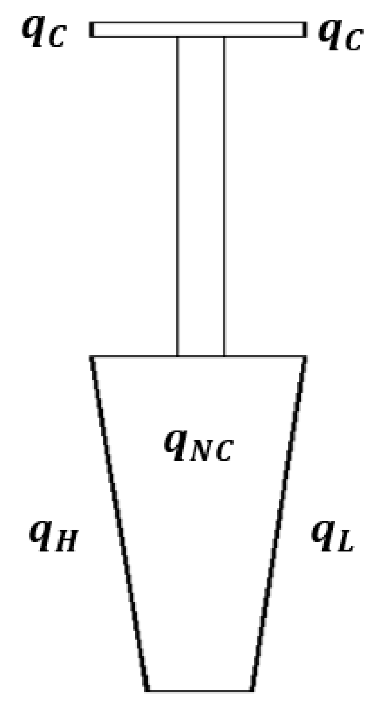
2.1. Cyclic Symmetry
- −
- EN is an N × N Fourier matrix (N is the number of blocks, coincident with the number of nodal diameters h in this case), and is its conjugate transpose.
- −
- IP is the identity matrix of dimension P, P being the dimension of each block of matrix KBD.
- −
- ⊗ is the Kronecker product.
2.2. Craig–Bampton Method
3. Reduction Methods for Bladed Disks
3.1. Direct Method
3.2. Two-Step Method
3.3. Remarks about the Two Approaches
- The direct method requires one reduction ( matrix) for each harmonic index h, while the two-step method requires a first reduction ( matrix), which is performed only once, followed by a second reduction ( matrix) for each harmonic index.
- The direct method requires a lower number of constraint modes to be computed with respect to the two-step method, where the number of static analyses necessary to generate the constraint modes is proportional to the number of contact dofs and to the number of inter-sector interface dofs.
- In the direct method, the linear modal analyses (one per each harmonic index h, necessary to compute the fixed-interface modes , are computed on the full model of the fundamental sector. In the two-step method, only one modal analysis of the full model of the fundamental sector is performed to obtain , and the modal analyses performed in the second reduction operate on an already reduced model.
- Fixed-interface modes computed with the direct method respect the cyclic symmetry properties of the bladed disk, while fixed-interface modes assume fixed inter-sector interfaces.
4. Numerical Results
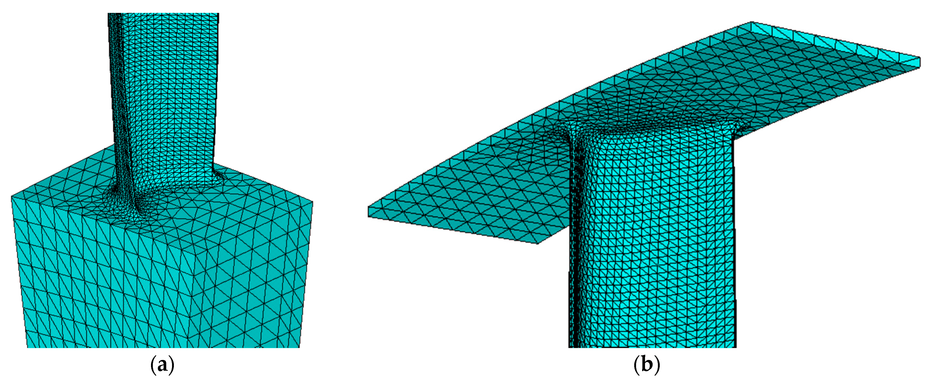
4.1. First Test Cases for Accuracy and Efficiency Analysis
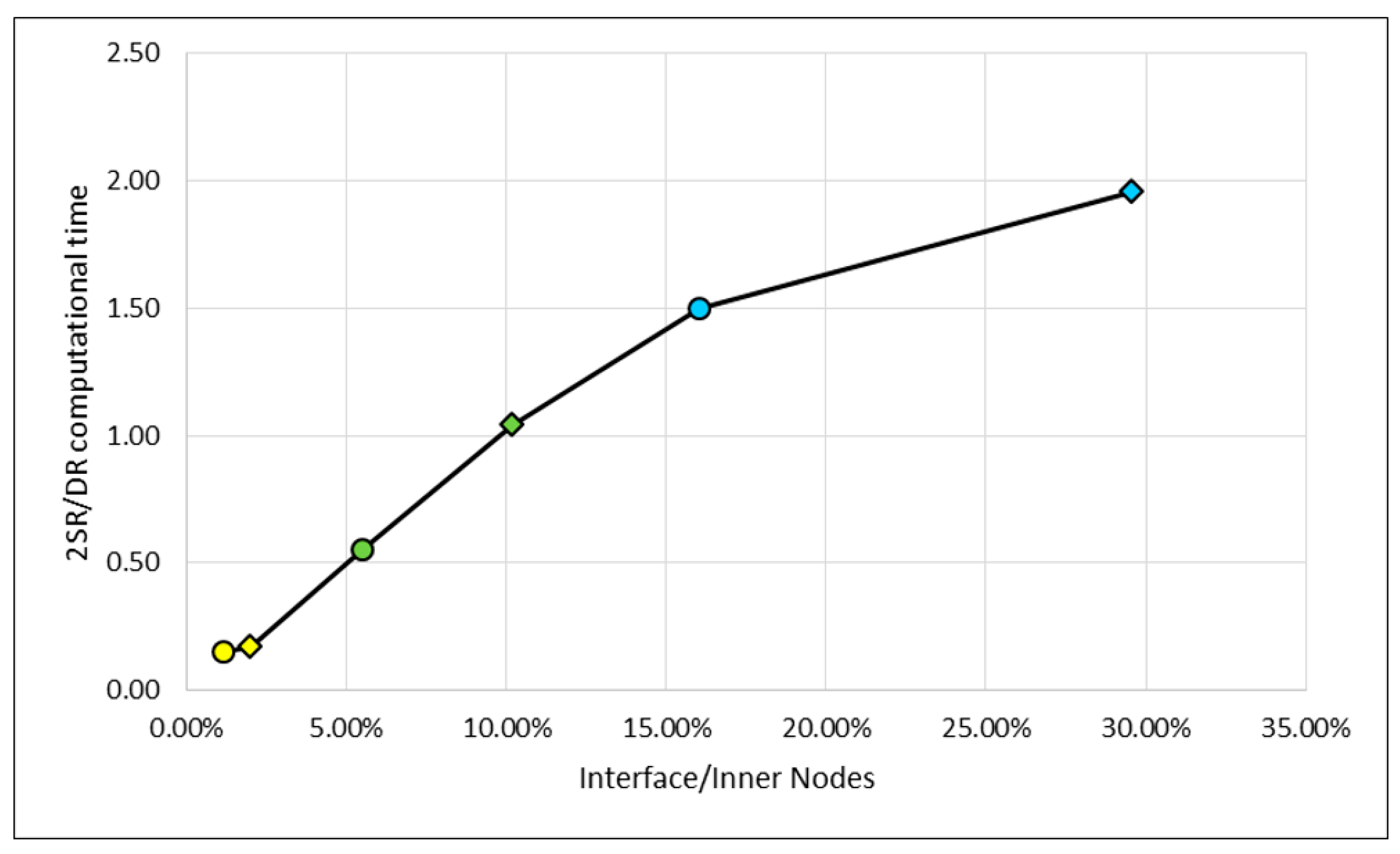
4.2. Additional Test Case for Efficiency Analysis.
- the calculation of the constraint modes in the 1st step is the most time-consuming operation in the two-step process,
- the computation of the fixed-interface modes is the most time-consuming step of the direct method.
5. Conclusions
Author Contributions
Funding
Conflicts of Interest
References
- Seinturier, E. Forced Response Computation for Bladed Disks: Industrial Practices and Advanced Methods. In Proceedings of the 12th IFToMM World Congress, Besançon, France, 18–21 June 2007. [Google Scholar]
- Krack, M.; Salles, L.; Thouverez, F. Vibration Prediction of Bladed Disks Coupled by Friction Joints. Arch. Comput. Meth. Eng. 2017, 3, 589–636. [Google Scholar] [CrossRef]
- Siewert, C.; Panning, L.; Wallaschek, J.; Richter, C. Multiharmonic Forced Response Analysis of a Turbine Blading Coupled by Nonlinear Contact Forces. J. Eng. Gas Turbines Power 2010, 132, 082501. [Google Scholar] [CrossRef]
- Zucca, S.; Gola, M.M.; Piraccini, F. Non-Linear Dynamics of Steam Turbine Blades with Shroud: Numerical Analysis and Experiments. In Proceedings of the ASME Turbo Expo 2012, Copenhagen, Denmark, 11–15 June 2012; p. 665. [Google Scholar] [CrossRef]
- Zucca, S.; Di Maio, D.; Ewins, D.J. Measuring the performance of underplatform dampers for turbine blades by rotating laser Doppler Vibrometer. Mech. Syst. Sig. Process. 2012, 32, 269–281. [Google Scholar] [CrossRef]
- Botto, D.; Umer, M. A novel test rig to investigate under-platform damper dynamics. Mech. Syst. Sig. Process. 2018, 100, 344–359. [Google Scholar] [CrossRef]
- Pesaresi, L.; Salles, L.; Jones, A.; Green, J.S.; Schwingshackl, C.W. Modelling the nonlinear behaviour of an underplatform damper test rig for turbine applications. Mech. Syst. Sig. Process. 2017, 85, 662–679. [Google Scholar] [CrossRef]
- Petrov, E.P.; Ewins, D.J. Effects of Damping and Varying Contact Area at Blade-Disk Joints in Forced Response Analysis of Bladed Disk Assemblies. J. Turbomach. 2005, 128, 403–410. [Google Scholar] [CrossRef]
- Zucca, S.; Firrone, C.M.; Gola, M.M. Numerical assessment of friction damping at turbine blade root joints by simultaneous calculation of the static and dynamic contact loads. Nonlinear Dyn. 2012, 67, 1943–1955. [Google Scholar] [CrossRef]
- Laxalde, D.; Thouverez, F.; Lombard, J.-P. Forced Response Analysis of Integrally Bladed Disks With Friction Ring Dampers. J. Vib. Acoust. 2010, 132, 011013. [Google Scholar] [CrossRef]
- Tang, W.; Epureanu, B.I. Nonlinear dynamics of mistuned bladed disks with ring dampers. Int. J. Non Linear Mech. 2017, 97, 30–40. [Google Scholar] [CrossRef]
- Battiato, G.; Firrone, C.M.; Berruti, T.M.; Epureanu, B.I. Reduced Order Modeling for Multi-Stage Bladed Disks With Friction Contacts at the Flange Joint. In Proceedings of the ASME Turbo Expo 2017: Turbomachinery Technical Conference and Exposition, Charlotte, NC, USA, 26–30 June 2017; p. V07BT35A027. [Google Scholar] [CrossRef]
- Lavella, M.; Botto, D.; Gola, M.M. Test Rig for Wear and Contact Parameters Extraction for Flat-on-Flat Contact Surfaces. In Proceedings of the ASME/STLE 2011 International Joint Tribology Conference, Los Angeles, CA, USA, 24–26 October 2011; pp. 307–309. [Google Scholar] [CrossRef]
- Schwingshackl, C.W.; Petrov, E.P.; Ewins, D.J. Measured and estimated friction interface parameters in a nonlinear dynamic analysis. Mech. Syst. Sig. Process. 2012, 28, 574–584. [Google Scholar] [CrossRef]
- Cardona, A.; Coune, T.; Lerusse, A.; Geradin, M. A multiharmonic method for non-linear vibration analysis. Int. J. Numer. Methods Eng. 1994, 37, 1593–1608. [Google Scholar] [CrossRef]
- Thomas, D.L. Dynamics of Rotationally Periodic Structures. Int. J. Numer. Methods Eng. 1979, 14, 81–102. [Google Scholar] [CrossRef]
- Castanier, M.P.; Pierre, C. Modeling and Analysis of Mistuned Bladed Disk Vibration: Current Status and Emerging Directions. J. Propul. Power 2006, 22, 384–396. [Google Scholar] [CrossRef]
- Grolet, A.; Thouverez, F. Free and forced vibration analysis of a nonlinear system with cyclic symmetry: Application to a simplified model. J. Sound Vib. 2012, 331, 2911–2928. [Google Scholar] [CrossRef]
- Mitra, M.; Zucca, S.; Epureanu, B.I. Effects of Contact Mistuning on Shrouded Blisk Dynamics. In Proceedings of the ASME Turbo Expo 2016: Turbomachinery Technical Conference and Exposition, Seoul, Korea, 13–17 June 2016; p. V07AT32A026. [Google Scholar] [CrossRef]
- Olson, B.J.; Shaw, S.W.; Shi, C.; Pierre, C.; Parker, R.G. Circulant Matrices and Their Application to Vibration Analysis. Appl. Mech. Rev. 2014, 66, 040803. [Google Scholar] [CrossRef]
- Craig, R.R.; Bampton, M.C.C. Coupling of substructures for dynamic analyses. AIAA J. 1968, 6, 1313–1319. [Google Scholar] [CrossRef]
- Bladh, R.; Castanier, M.P.; Pierre, C. Component-Mode-Based Reduced Order Modeling Techniques for Mistuned Bladed Disks—Part I: Theoretical Models. J. Eng. Gas Turbines Power 2001, 123, 89–99. [Google Scholar] [CrossRef]


| Test Case | A | B | ||
|---|---|---|---|---|
| Blades | 27 | 81 | ||
| Sector |  |  | ||
| Element Type | Linear | Quadratic | Linear | Quadratic |
| Elements | 16,561 | 16,561 | 5627 | 5627 |
| Nodes | 6052 | 30,920 | 2454 | 11,672 |
| Direct Method | Two-Step Method | ||
|---|---|---|---|
| 1st Set of ROMs | 2nd Set of ROMs | 3rd Set of ROMs | |
| Z | (Z1; Z2) | (Z1; Z2) | (Z1; Z2) |
| 20 | 60; 20 | 120; 20 | 180; 20 |
| 40 | 60; 40 | 120; 40 | 180; 40 |
| 60 | 60; 60 | 120; 60 | 180; 60 |
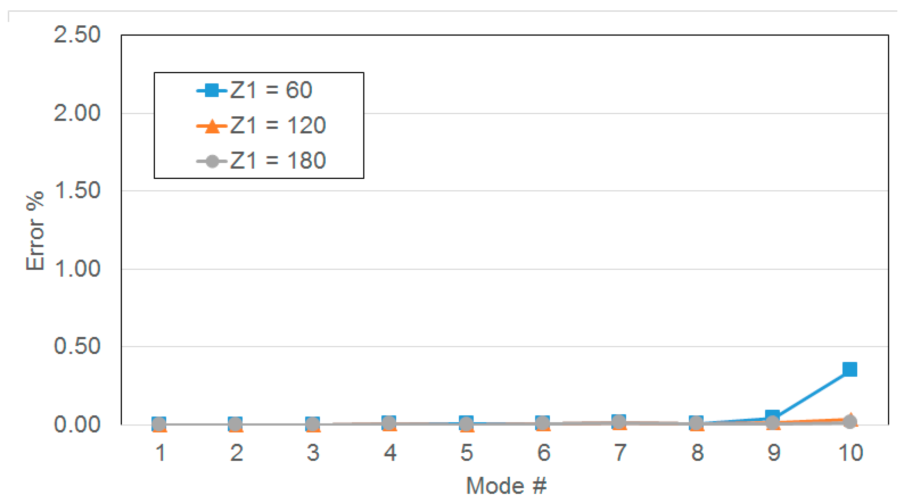
| Full | Direct Method | Two-Step Method | ||||||||||
|---|---|---|---|---|---|---|---|---|---|---|---|---|
| (Hz) | Z1 = 60 | Z1 = 120 | Z1 = 180 | |||||||||
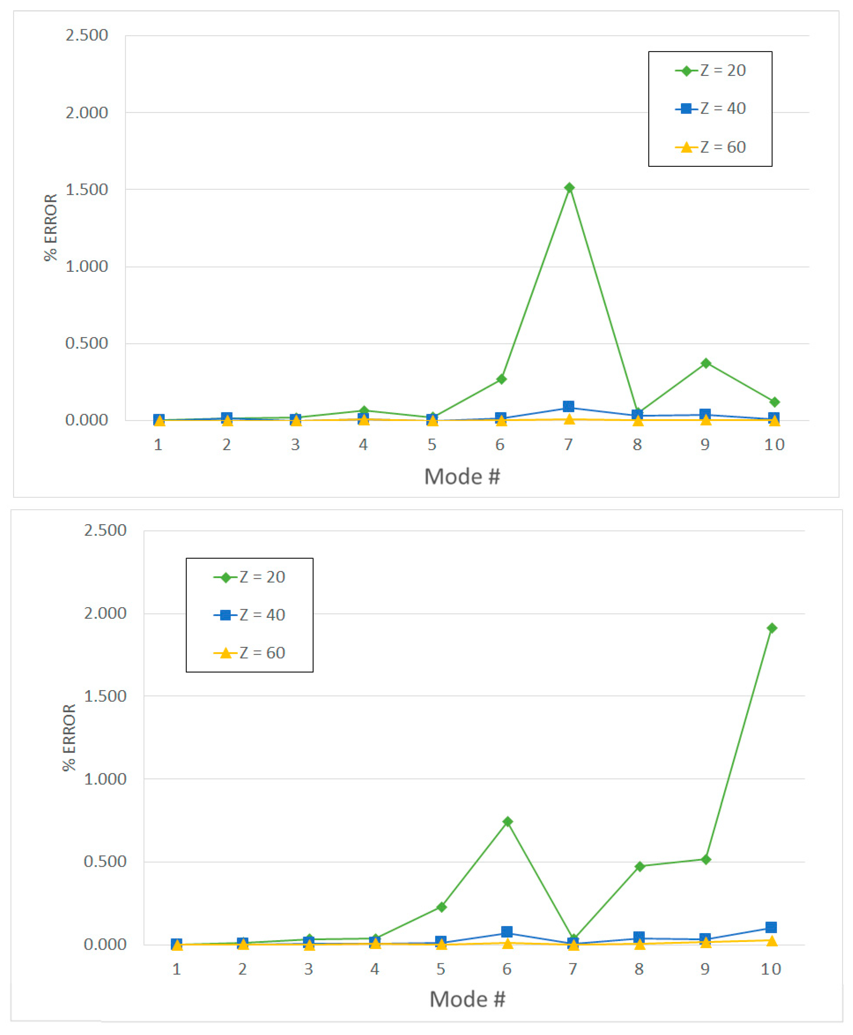
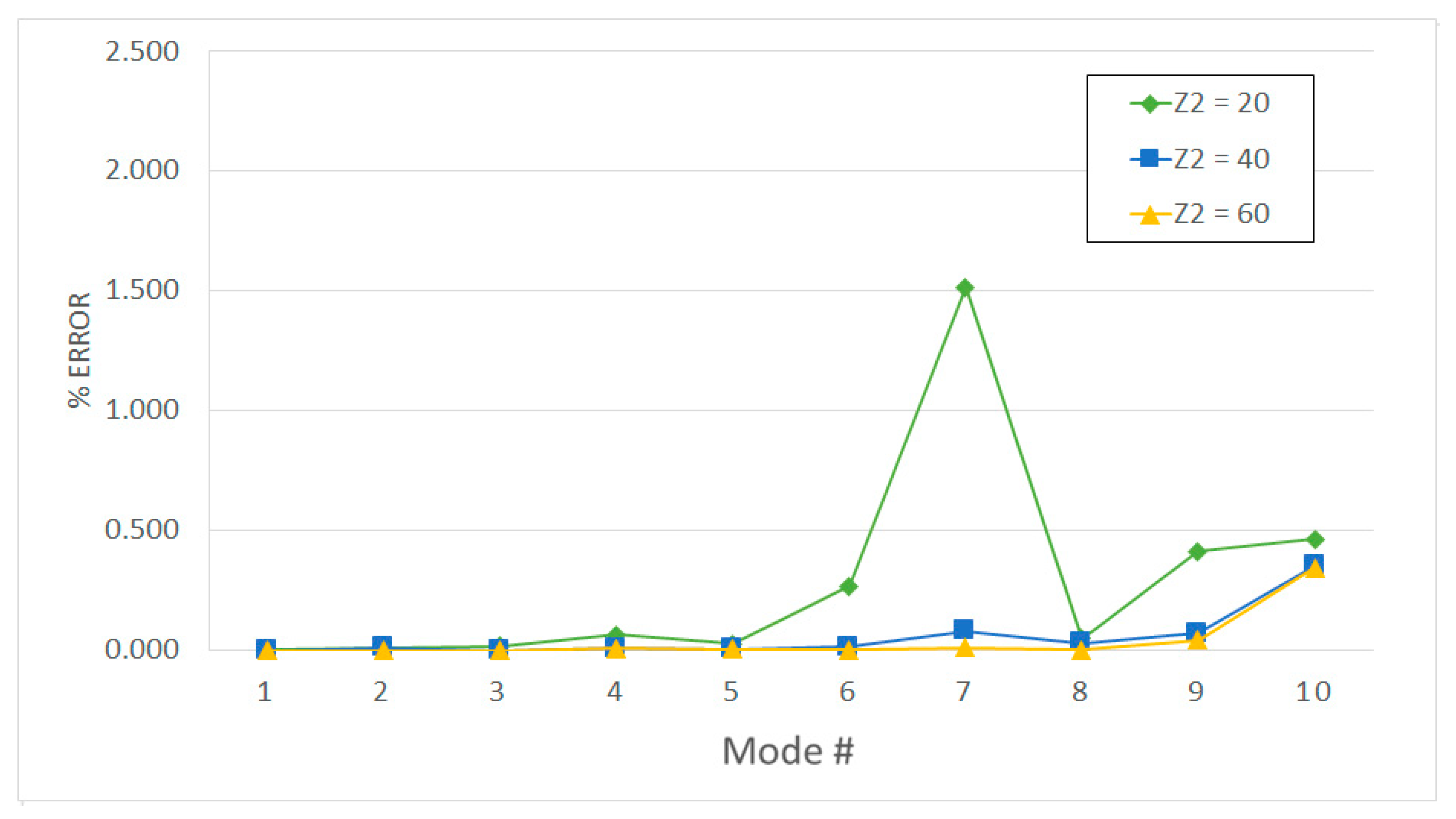
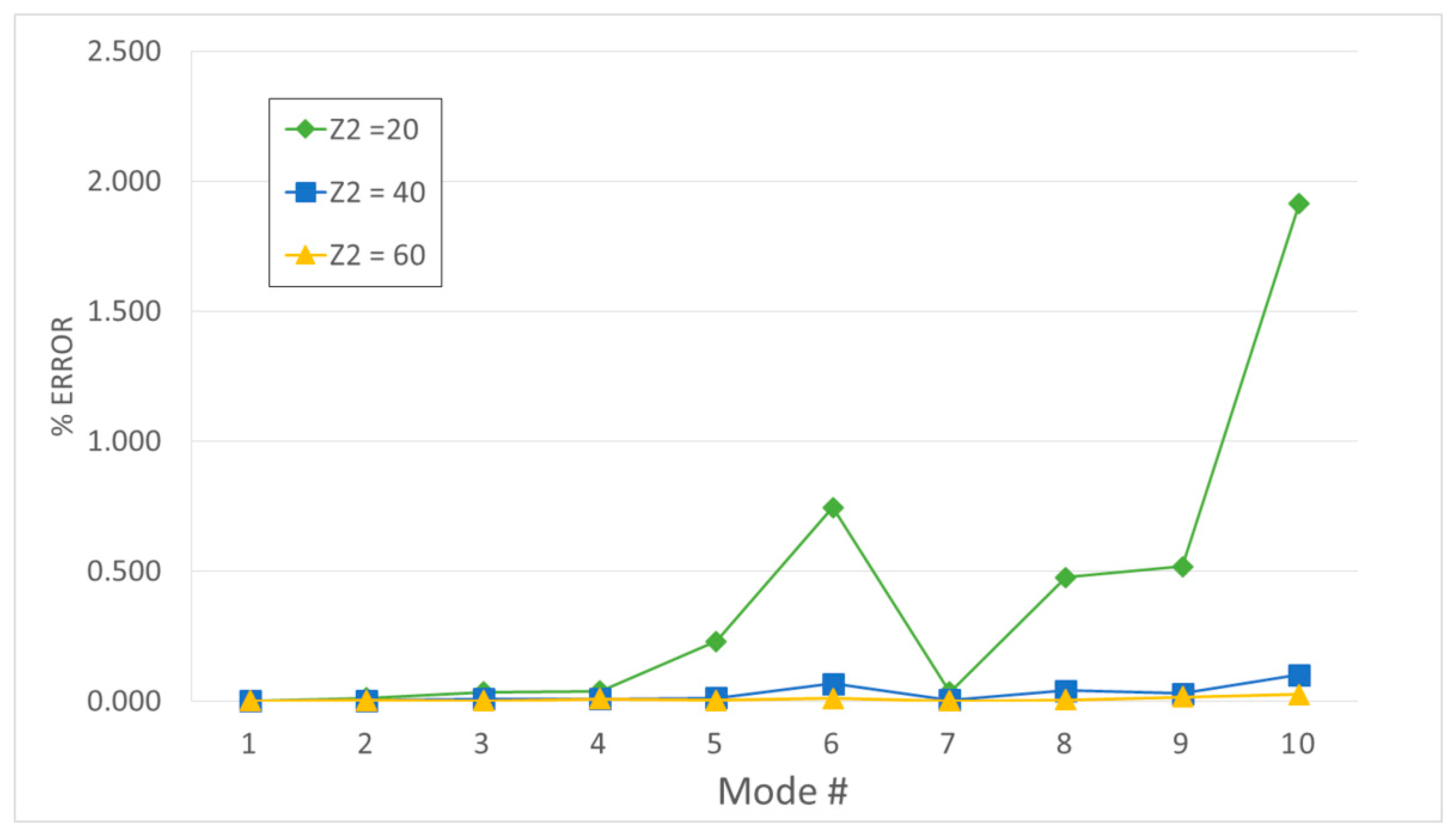
| Z = 20 | Z = 40 | Z = 60 | Z2 = 20 | Z2 = 40 | Z2 = 60 | Z2 = 20 | Z2 = 40 | Z2 = 60 | Z2 = 20 | Z2 = 40 | Z2 = 60 | |
| 200.18 | 0.00% | 0.00% | 0.00% | 0.00% | 0.00% | 0.00% | 0.00% | 0.00% | 0.00% | 0.00% | 0.00% | 0.00% |
| 488.70 | 0.01% | 0.01% | 0.00% | 0.01% | 0.01% | 0.00% | 0.01% | 0.01% | 0.00% | 0.01% | 0.01% | 0.00% |
| 1044.80 | 0.02% | 0.00% | 0.00% | 0.02% | 0.00% | 0.00% | 0.02% | 0.00% | 0.00% | 0.02% | 0.00% | 0.00% |
| 1211.40 | 0.07% | 0.01% | 0.01% | 0.07% | 0.01% | 0.01% | 0.07% | 0.01% | 0.01% | 0.07% | 0.01% | 0.01% |
| 1943.90 | 0.02% | 0.00% | 0.00% | 0.03% | 0.01% | 0.01% | 0.03% | 0.01% | 0.00% | 0.03% | 0.00% | 0.00% |
| 3439.40 | 0.27% | 0.01% | 0.00% | 0.27% | 0.01% | 0.00% | 0.27% | 0.01% | 0.00% | 0.27% | 0.01% | 0.00% |
| 3895.00 | 1.51% | 0.08% | 0.01% | 1.51% | 0.08% | 0.01% | 1.51% | 0.08% | 0.01% | 1.51% | 0.08% | 0.01% |
| 6389.70 | 0.05% | 0.03% | 0.00% | 0.05% | 0.03% | 0.00% | 0.05% | 0.03% | 0.00% | 0.05% | 0.03% | 0.00% |
| 6915.70 | 0.37% | 0.03% | 0.01% | 0.41% | 0.07% | 0.04% | 0.38% | 0.04% | 0.01% | 0.37% | 0.04% | 0.01% |
| 7775.40 | 0.12% | 0.01% | 0.00% | 0.46% | 0.35% | 0.34% | 0.16% | 0.04% | 0.03% | 0.13% | 0.02% | 0.01% |
| Test Case | Node # | Direct (s) | Two-Step (s) | Two-Step/Direct |
|---|---|---|---|---|
| B-Lin | 2454 | 328 | 641 | 1.95 |
| B-Quad | 6052 | 779 | 1169 | 1.50 |
| A-Lin | 11,672 | 322 | 336 | 1.04 |
| A-Quad | 30,920 | 1120 | 620 | 0.55 |
| Test Case | Node # | Direct (s) | Two-Step (s) | Two-Step/Direct |
|---|---|---|---|---|
| B-Lin | 2454 | 328 | 641 | 1.95 |
| B-Quad | 6052 | 779 | 1169 | 1.50 |
| A-Lin | 11,672 | 322 | 336 | 1.04 |
| C-Lin | 13,885 | 646 | 110 | 0.17 |
| A-Quad | 30,920 | 1120 | 620 | 0.55 |
| C-Quad | 89,228 | 2244 | 332 | 0.15 |
© 2018 by the authors. Licensee MDPI, Basel, Switzerland. This article is an open access article distributed under the terms and conditions of the Creative Commons Attribution (CC BY) license (http://creativecommons.org/licenses/by/4.0/).
Share and Cite
Sommariva, A.; Zucca, S. A Comparison between Two Reduction Strategies for Shrouded Bladed Disks. Appl. Sci. 2018, 8, 1736. https://doi.org/10.3390/app8101736
Sommariva A, Zucca S. A Comparison between Two Reduction Strategies for Shrouded Bladed Disks. Applied Sciences. 2018; 8(10):1736. https://doi.org/10.3390/app8101736
Chicago/Turabian StyleSommariva, Alessandro, and Stefano Zucca. 2018. "A Comparison between Two Reduction Strategies for Shrouded Bladed Disks" Applied Sciences 8, no. 10: 1736. https://doi.org/10.3390/app8101736
APA StyleSommariva, A., & Zucca, S. (2018). A Comparison between Two Reduction Strategies for Shrouded Bladed Disks. Applied Sciences, 8(10), 1736. https://doi.org/10.3390/app8101736