A Modal Solution for Finite Length Rods with Non-Uniform Area

Abstract

This paper derives a modal solution to the displacement field of a finite length rod whose area varies with respect to its length. This new method facilitates a solution to any problem where the area and derivative of the area can be represented as analytical functions. The problem begins by writing the longitudinal displacement of the non-uniform area rod as a series of indexed coefficients multiplied by the eigenfunctions of the uniform area rod. This series solution is inserted into the non-uniform area rod equation and multiplied by a single p-indexed eigenfunction. This equation is then integrated over the interval of the rod. Although the resultant expressions are not orthogonal, they can be written as a set of linear algebraic equations which can be solved to yield the unknown coefficients. Once these are known, the displacement of the system can be calculated. Five example problems are included: the first one has a non-uniform area that corresponds with a known analytical solution, the second has an area that can be represented by a Fourier series, the third and fourth have areas that do not have a known analytical solution and the fifth is a generic second order non-constant coefficient differential equation. Four of these problems are verified with other methods. Convergence of the series solution is discussed. It is shown that this new model is almost two orders of magnitude faster than corresponding finite element analysis.

1. Introduction

Rods (or bars) are common mechanical elements in the automotive, aerospace, construction and maritime industries. Modeling their behavior is important so that the appropriate static and dynamic response can be incorporated into a design. Modeling also allows an understanding of the vibrational response of these systems before they are built so that costly prototyping can be minimized or avoided altogether. Increased knowledge of these systems allows designers to incorporate features and characteristics that might not be understood and omitted from the initial design. Modeling of these systems started with the basic rod equation [1], which is sometimes referred to as elementary theory, and this governing second order differential equation is the focus of this work. This system can be modeled by differential equations that contain higher order effects and this usually includes some form of transverse motion or rotation. These models include Love (or Rayleigh-Love) theory [2], Mindlin-Herrmann theory [2], three mode theory [2], Rayleigh-Bishop theory [3] and fully elastic theory [4]. These higher order models are typically used for rods with relatively large cross-sectional areas or higher frequency ranges where additional dynamic effects need to be included in the differential equations to properly capture the dynamics of the rod. These higher order models are not discussed further in this paper.

The problem of the rod with uniform area has been addressed by many authors [1,5,6]. The rod problem with classical boundary conditions (free-free, free-fixed or fixed-fixed) is present in almost all vibration textbooks. A standard solution method for this problem is the finite sine (or cosine) transform [7]. Boundary conditions that are not classical are also possible, and these can include translational springs [6,8] and dampers [9]. Different analytical methods have been developed to solve these specific problems, typically modeling rods with uniform area.

The problem of the rod with non-uniform area has been studied by numerous authors. Many of these papers involve modeling a rod whose functional form of cross-sectional area lends itself to an exact analytical solution to the problem. Tsui [10] investigated a finite length rod whose cross-sectional area was equal to the spatial position raised to a constant exponent and showed that this results in a standard Bessel equation solution. Spyrakos and Chen [11] derived the dynamic and stiffness matrices of a rod with a polynomial taper using power series expansions of Bessel functions. This analysis was concentrated on linear and quadratic area changes. Abrate [12] showed that if the rod had an area change proportional to a second order polynomial, the problem could be transformed into the equation for a uniform rod. Furthermore, this paper developed a Rayleigh-Ritz approximation method for a beam where the approximating functions were polynomials satisfying the boundary condition at x = 0. This method does not allow the approximating function to satisfy the boundary condition at x = L. Kumar and Sujith [13] showed that for rods with polynomial and sinusoidal area variation, the problem could be transformed into an analytically solvable standard differential equation. Li [14] analyzed multistep rods that contained variations of the area, stiffness and mass as functions of polynomials and exponentials and calculated the corresponding natural frequencies and mode shapes. This method was further extended [15] to include the transfer matrix method to determine natural frequencies of multistep rods. Raj and Sujith [16] solved this problem where the rod’s area variation yielded solutions that were confluent hypergeometric functions. The functional form of the area in this work is typically an exponential function multiplied by the spatial variable to a real power. Lee et al. [17] studied this problem using a wave approach for the reflection, transmission and propagation of longitudinal waves for uniform, linear and conical change of area. Han et al. [3] developed a transfer matrix method to understand the propagation characteristics of a rod with variable cross-section. They utilized Hamilton’s principle to derive and solve the equations of motion for a rod with an exponential and a polynomial shape and applied this analysis to higher order rod theory. Brun et al. [18] derived asymptotic approximations for solutions of Bloch waves for finite and infinite length structures and applied this analysis to slender elastic structures. Brun et al. [19] also investigated transfer function matrix methods for systems with structural interfaces and this method could be applied to a rod with a piece-wise constant cross-section.

Asymptotic methods have been extensively applied to this problem [20] using variational and asymptotic approaches. These methods have been applied to a rod with circular [21] cross section and the resulting dispersion curve and spectrum were calculated. They were also applied to Timoshenko type rods [22] to determine the shear coefficients of circular, annular, elliptical and square rods. These variational methods have also been extended to transverse motion of isotropic centrally symmetric beams [23] and anisotropic closed cross section beams [24], however, transverse motion is beyond the scope of this paper and is not investigated herein. Finally, it is noted [25] that the theory of an area change can be extended to the theory of a change in the material properties of the medium.

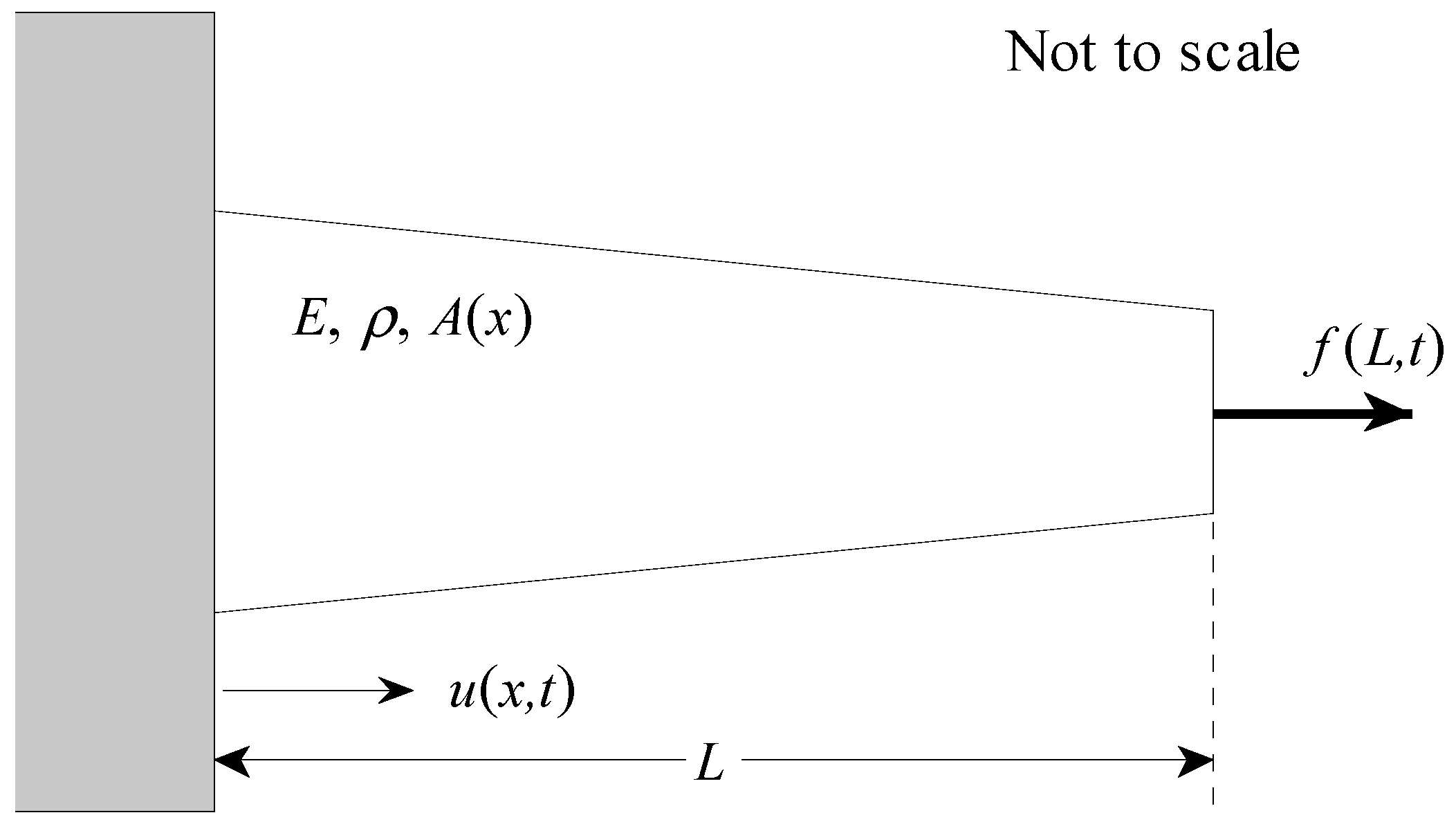
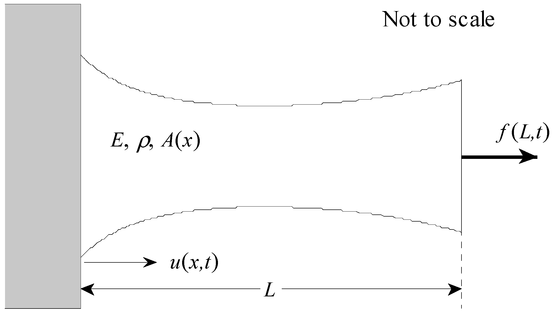
This paper derives a modal solution to the displacement field of a finite length rod whose area varies with respect to its length. This new analysis method is explicitly designed to calculate series solutions to this problem where no analytical solution currently exists. This allows the displacement field to be calculated for any problem where the area and derivative of the area can be represented as analytical functions. The specific problem of a linear change of area is shown in Figure 1 with the boundary condition at x = 0 fixed and the boundary condition at x = L free. Different combinations of these boundary conditions and different functional forms for change of area are possible and these are discussed and analyzed in detail below. The solution begins by writing the displacement field as an n-indexed series solution of an unknown indexed wave propagation coefficient multiplied by the eigenfunction of the uniform area rod. This expression is inserted into the differential equation of the non-uniform area rod that contains a restoring force term, an inertial force term and an area change force term. The resulting expression is then multiplied by a p-index expression that is the eigenfunction of the uniform area rod and integrated over the length of the rod. This results in an infinite set of linear algebraic equations that can be truncated and solved to yield the wave propagation coefficients. Once these are known, the system displacements can be determined. Five different example problems are generated and four of them are checked using other analytical or numerical methods.

2. Methods

The system under consideration is a finite length rod with changes in its area with respect to the longitudinal position. This problem is analytically modeled using the rod longitudinal differential equation. The model uses the following assumptions: (1) the excitation is at a fixed frequency; (2) the displacement field is one-dimensional in the longitudinal direction; (3) the (varying) height and width of the rod are small compared to its length; (4) the rod has uniform stress distribution; (5) the area can be represented as a strictly positive continuous analytical function with respect to position on the interval of the rod and has a continuous first derivative; (6) the change of area is symmetric about the centroid of the rod; and (7) the particle motion is linear. The rod longitudinal motion equation with non-uniform area is [1]

$$EA(x)\frac{{\partial }^{2}u(x,t)}{\partial x^2}+E\frac{\partial A(x)}{\partial x}\frac{\partial u(x,t)}{\partial x}-\rho A(x)\frac{{\partial }^{2}u(x,t)}{\partial t^2}=f(x,t),$$

(1)

where $u(x,t)$ is longitudinal displacement, x is spatial position, t is time, E is Young’s modulus, $A(x)$ is the cross-sectional area, ρ is density and $f(x,t)$ is the applied force per unit length in the longitudinal direction. Note the second term in Equation (1) that is present because of the spatially varying area. This term is the longitudinal stress in the rod multiplied by the change of area with respect to the spatial variable x. The forcing function and the displacement are modeled as harmonic in time at fixed frequency, i.e., $u(x,t)=U(x)\exp (-\mathrm{i}\omega t)$ and $f(x,t)=F(x)\exp (-\mathrm{i}\omega t)$, which transforms Equation (1) into

$$EA(x)\frac{{\mathrm{d}}^{2}U(x)}{\mathrm{d}{x}^2}+E\frac{\mathrm{d}A(x)}{\mathrm{d}x}\frac{\mathrm{d}U(x)}{\mathrm{d}x}+\rho {\omega }^{2}A(x)U(x)=F(x).$$

(2)

This is a second order ordinary linear differential equation with non-constant coefficients. To facilitate a solution to this problem, it is necessary to specify boundary conditions. For this method, three possible combinations of boundary conditions are possible: (1) fixed-fixed, (2) fixed-free or (3) free-free. The eigenfunctions (or modes) for this problem with the rod having a uniform cross-sectional area are the basis for this solution method, and for the fixed-fixed boundary condition these are

$${\phi }_n(x)=\sin \left(\frac{n\pi x}{L}\right)n=1,2,3\cdots ,$$

(3)

for the fixed-free boundary condition they are

$${\phi }_n(x)=\sin \left[\frac{(2n-1)\pi x}{2L}\right]n=1,2,3\cdots ,$$

(4)

and for the free-free boundary condition they are

$${\phi }_n(x)=\cos \left(\frac{n\pi x}{L}\right)n=0,1,2,3\cdots .$$

(5)

The solution to the longitudinal displacement is now written as a series of indexed coefficients multiplied by the eigenfunctions from the uniform area differential equation. This equation, for the fixed-free boundary condition, is

$$U(x)={\displaystyle \sum _{n=1}^{n=\infty }{U}_n\sin \left[\frac{(2n-1)\pi x}{2L}\right]},$$

(6)

where $U_n$ is the unknown wave propagation coefficient whose solution is sought. The fixed-free boundary condition is analyzed in this section as it corresponds to the example problems presented later in the paper. Equation (6) is now inserted into Equation (2), and this results in

$$\begin{array}{l}A(x){\displaystyle \sum _{n=1}^{n=\infty }\left\{\rho {\omega }^2-E{\left[\frac{(2n-1)\pi }{2L}\right]}^2\right\}{U}_n\sin \left[\frac{(2n-1)\pi x}{2L}\right]}+\\ E\frac{\mathrm{d}A(x)}{\mathrm{d}x}{\displaystyle \sum _{n=1}^{n=\infty }\left[\frac{(2n-1)\pi }{2L}\right]U_n\cos \left[\frac{(2n-1)\pi x}{2L}\right]}=F(x).\end{array}$$

(7)

Equation (7) is now multiplied by a single p-indexed eigenfunction, which yields

$$\begin{array}{l}A(x){\displaystyle \sum _{n=1}^{n=\infty }\left\{\rho {\omega }^2-E{\left[\frac{(2n-1)\pi }{2L}\right]}^2\right\}{U}_n\sin \left[\frac{(2n-1)\pi x}{2L}\right]}\sin \left[\frac{(2p-1)\pi x}{2L}\right]+\\ E\frac{\mathrm{d}A(x)}{\mathrm{d}x}{\displaystyle \sum _{n=1}^{n=\infty }\left[\frac{(2n-1)\pi }{2L}\right]U_n\cos \left[\frac{(2n-1)\pi x}{2L}\right]}\sin \left[\frac{(2p-1)\pi x}{2L}\right]=F(x).\end{array}$$

(8)

Equation (8) is integrated on [0,L], and written multiple times using values of p from 1 to infinity, which produces the matrix equation

$$\left[\mathbf{G}+\mathbf{H}\right]\mathbf{u}=\mathbf{f},$$

(9)

where

$$G_{p,n}={\displaystyle \underset{0}{\overset{L}{\int }}A(x)\left\{\rho {\omega }^2-E{\left[\frac{(2n-1)\pi }{2L}\right]}^2\right\}\sin \left[\frac{(2n-1)\pi x}{2L}\right]\sin \left[\frac{(2p-1)\pi x}{2L}\right]}\mathrm{d}x,$$

(10)

$$H_{p,n}={\displaystyle \underset{0}{\overset{L}{\int }}E\frac{\mathrm{d}A(x)}{\mathrm{d}x}\left[\frac{(2n-1)\pi }{2L}\right]\cos \left[\frac{(2n-1)\pi x}{2L}\right]\sin \left[\frac{(2p-1)\pi x}{2L}\right]}\mathrm{d}x,$$

(11)

$$u_{p,1}=U_p,$$

(12)

and

$$f_{p,1}={\displaystyle \underset{0}{\overset{L}{\int }}F(x)\sin \left[\frac{(2p-1)\pi x}{2L}\right]\mathrm{d}x}.$$

(13)

Note that Equations (10) and (11) are inner products with a weight function of the area (Equation (10)) and the derivative of the area (Equation (11)), however, they are not (in general) orthogonal. Thus, for problems where the rod area is non-uniform, G and H will be full matrices. Physically, these equations establish that the modes are coupled to each other by the change of area of the rod. The matrix G represents the restoring and inertial forces and the matrix H represents the change of the amount of force as the area varies. For a finite number of terms in p and n, the wave propagation coefficients can be solved with

$$\mathbf{u}={\left[\mathbf{G}+\mathbf{H}\right]}^{-1}\mathbf{f}.$$

(14)

Once these are known, they can be inserted into Equation (6) to yield the displacements of the system.

3. Results

Four specific example problems applied to a rod are now generated and solved to illustrate this method. All of the problems analyzed are fixed-free rods with a harmonic point load applied to the free end. These problems have a linear variation, a triangular variation, a Bessel function variation and a Gamma function variation of the cross-sectional area. These problems are calculated using a set of parameters that result in a volume for each rod equal to 0.00324 m³ so that a comparison can be made between the different geometrical shapes. The parameter set that is constant is Young’s modulus E = 1 × 10⁷ N m⁻², density $\rho$ = 1200 kg m⁻³, rod length L = 3.0 m, rod width w = 0.03 m, applied spatial load location $x_f$ = 3.0 m, magnitude of applied spatial load $F_0$ = 1 N and location of the response $x_r$ = 2.25 m. The constants m and b are used to define the variation of the rod’s height. These values and units vary for each example problem and are listed in

Table 1. Values of the geometric parameters for specific rod shapes.

Rod Shape	m	Units of m	b	Units of b
Linear	−0.0080	dimensionless	0.0300	M
Triangular	0.0040	m	0.0280	M
Bessel	0.7500	m−1	0.0277	M
Gamma	0.0800	m−1	0.0120	M

. The solution to these problems is displacement versus frequency, and it is displayed graphically for the first five natural frequencies of the rod.

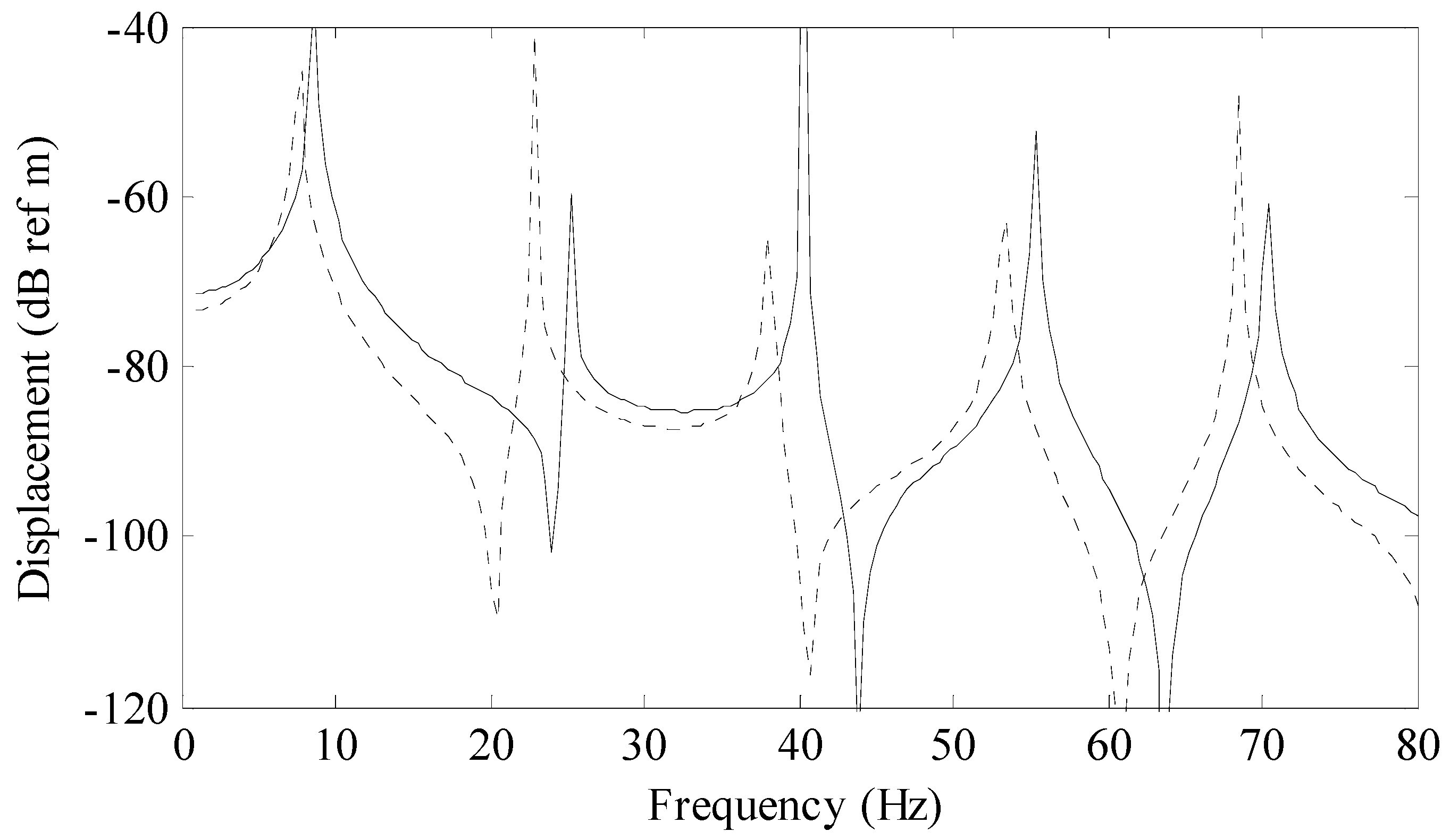
The first problem analyzed is a rod that has a linear variation in cross-sectional area, as shown in Figure 1. For this problem, the area is equal to

$$A(x)=2(mx+b)w>0\forall x\in [0,L],$$

(15)

and the derivative of the area with respect to the longitudinal variable is

$$\frac{\mathrm{d}A(x)}{\mathrm{d}x}=2mw.$$

(16)

The integrals from Equations (10), (11) and (13) are as follows

$$H_{p,n}=2w\left\{\rho {\omega }^2-E{\left[\frac{(2n-1)\pi }{2L}\right]}^2\right\}\left[\frac{bL}{2}+\frac{m{L}^2(4{\pi }^2{n}^2-4{\pi }^{2}n+{\pi }^2+4)}{4{\pi }^2{(2n-1)}^2}\right]p=n,$$

(17)

$$\begin{array}{l}{G}_{p,n}=2w\left\{\rho {\omega }^2-E{\left[\frac{(2n-1)\pi }{2L}\right]}^2\right\}\times \\ \left\{\frac{2m{L}^2\cos (n\pi )\cos (p\pi )[n^2-n+p^2-p+(1/2)]-m{L}^2(2n-1)(2p-1)}{2{\pi }^2{(-n^2+n+p^2-p)}^2}\right\}p\ne n,\end{array}$$

(18)

$$H_{p,n}=2wE\left[\frac{(2n-1)\pi }{2L}\right]\left[\frac{mL}{\pi (2n-1)}\right]p=n,$$

(19)

$$H_{p,n}=2wE\left[\frac{(2n-1)\pi }{2L}\right]\left\{\frac{mL[\cos (n\pi )\cos (p\pi )-2n\cos (n\pi )\cos (p\pi )+2p-1]}{2\pi (-n^2+n+p^2-p)}\right\}p\ne n$$

(20)

and

$$f_{p,1}=F_0\sin \left[\frac{(2p-1)\pi }{2}\right].$$

(21)

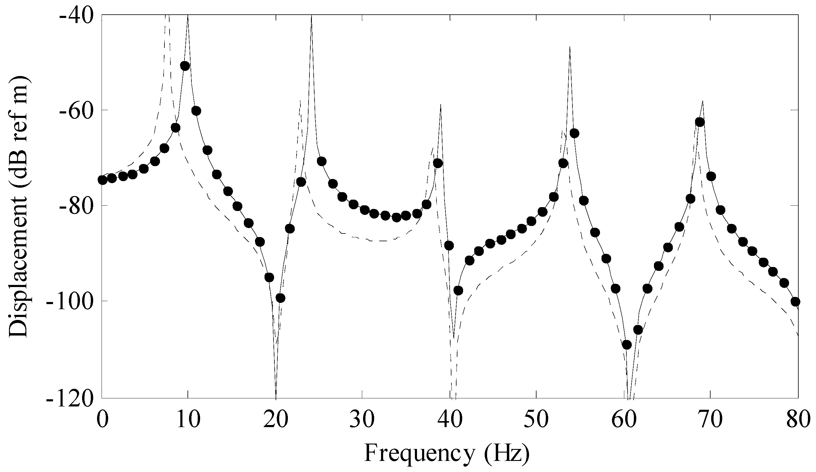
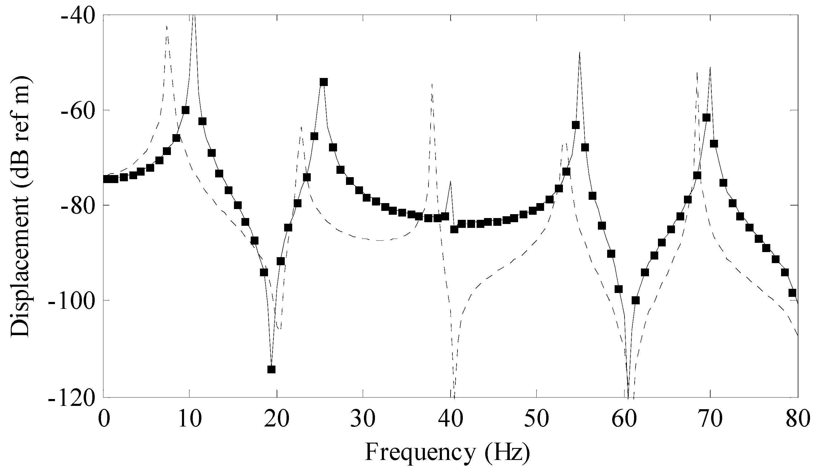
Figure 2 is a comparison of the series (modal) solution (solid line) to a previously derived analytical solution for a rod (circular markers) and a rod with uniform area (dashed line) called the baseline model. The series solution was calculated using 25 terms. The previously derived exact analytical solution is given by

$$\widehat{U}(x)=C_1{\mathrm{J}}_0\left[\kappa \left(\frac{b}{m}+x\right)\right]+C_2{\mathrm{Y}}_0\left[\kappa \left(\frac{b}{m}+x\right)\right],$$

(22)

where ${\mathrm{J}}_0$ denotes a zero order Bessel function of the first kind, ${\mathrm{Y}}_0$ denotes a zero order Bessel function of the second kind and

$$\kappa =\frac{\omega }{\sqrt{E/\rho }}.$$

(23)

The constants in Equation (22) are

$$C_1=\frac{-{\mathrm{Y}}_0\left[\kappa \left(\frac{b}{m}\right)\right]F_0}{2wE\kappa (mL+b)\left\{{\mathrm{Y}}_0\left[\kappa \left(\frac{b}{m}\right)\right]{\mathrm{J}}_1\left[\kappa \left(\frac{b}{m}+L\right)\right]-{\mathrm{J}}_0\left[\kappa \left(\frac{b}{m}\right)\right]{\mathrm{Y}}_1\left[\kappa \left(\frac{b}{m}+L\right)\right]\right\}}$$

(24)

and

$$C_2=\frac{{\mathrm{J}}_0\left[\kappa \left(\frac{b}{m}\right)\right]F_0}{2wE\kappa (mL+b)\left\{{\mathrm{Y}}_0\left[\kappa \left(\frac{b}{m}\right)\right]{\mathrm{J}}_1\left[\kappa \left(\frac{b}{m}+L\right)\right]-{\mathrm{J}}_0\left[\kappa \left(\frac{b}{m}\right)\right]{\mathrm{Y}}_1\left[\kappa \left(\frac{b}{m}+L\right)\right]\right\}}.$$

(25)

The baseline model was calculated with a standard finite sine transform where the height of the rod was a constant 0.018 m which produced a rod volume of 0.00324 m³.

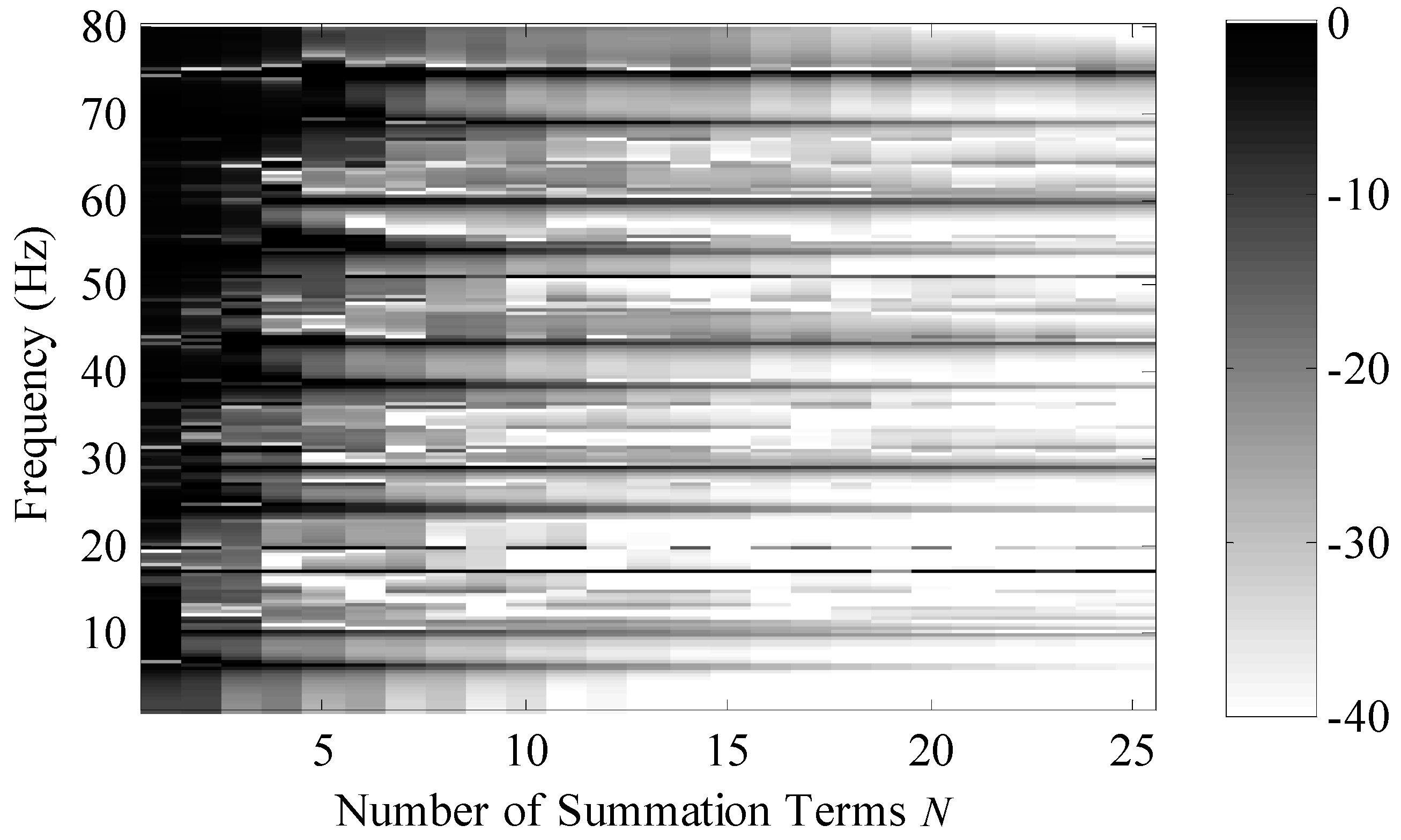
Convergence of the series in Equation (6) is an open issue as the rate of convergence is dependent on the model parameters, shape and change of shape of the rod. However, for the modeled systems presented in this paper, generalized statements can be deduced based on comparison of various solutions. Figure 3 is a plot of the convergence of the system versus number of summation terms and frequency. This convergence metric was calculated using the equation

$$C(N,f)=20{\log }_{10}\left[\frac{1}{J}{\displaystyle \sum _{j=1}^J\left|\frac{\widehat{U}(x_j)-U(x_j)}{\widehat{U}(x_j)}\right|}\right],$$

(26)

where $\widehat{U}(x_j)$ is the analytical solution, $U(x_j)$ is the series solution calculated using N terms, $x_j$ is the location of the jth calculation, J was equal to 15 and the spatial locations were equally spaced across the length of the rod. The region in white is −40 dB (or lower) and this corresponds to a one percent (or less) normalized difference between the two solutions. For this problem, one percent difference occurred when the normalized higher order wave propagation coefficients were −15.3 dB down on average across all frequency bins for this specific shape. In general, as frequency increases, more terms are needed for the series solution to converge.

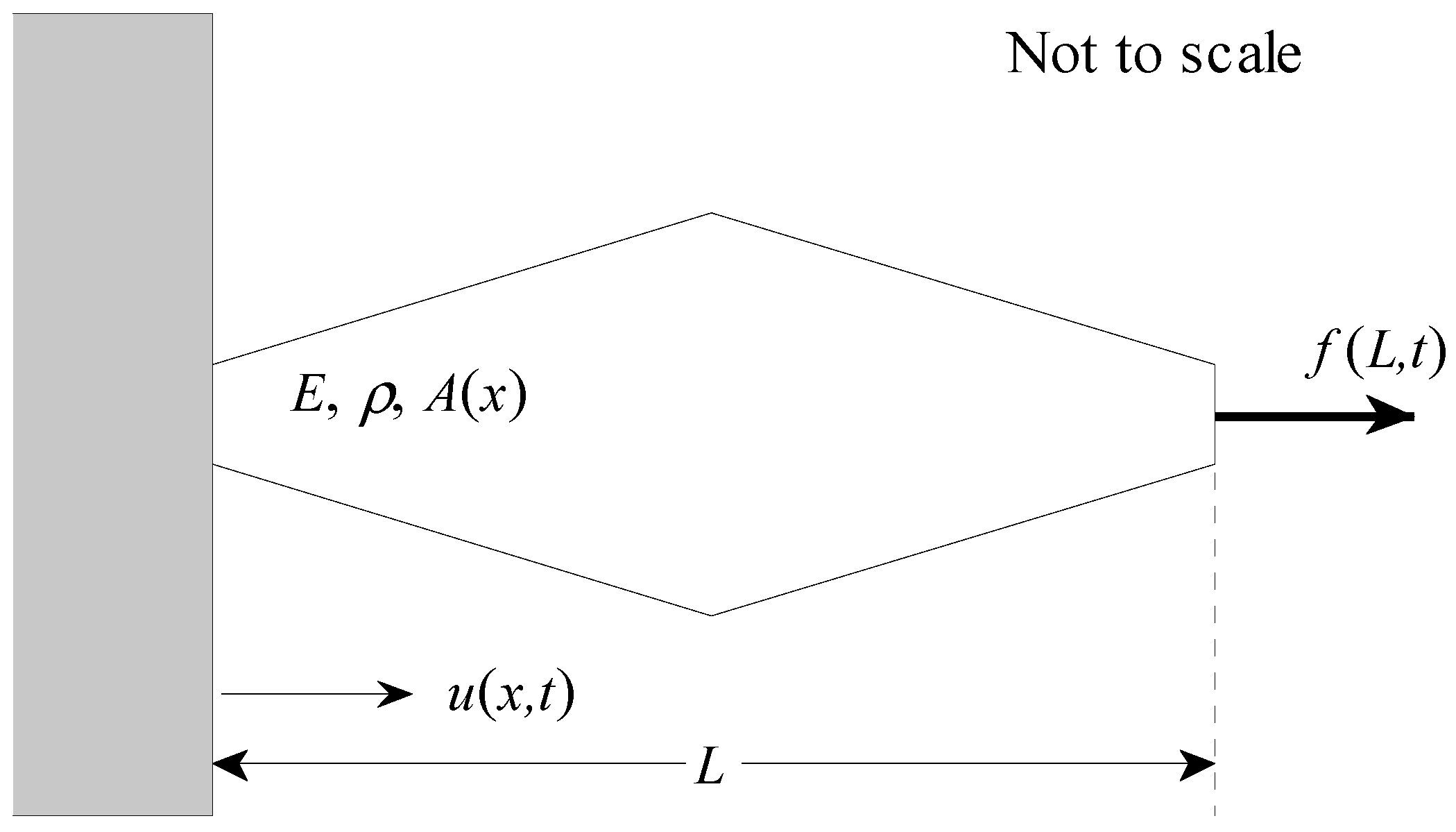
The second problem analyzed is a rod that has a triangular variation in cross-sectional area, as shown in Figure 4. For this problem, the area is approximated with a Fourier series and is written as

$$A(x)=2wb+2wm{\displaystyle \sum _{q=-Q}^{q=+Q}{c}_q\exp \left(\frac{\mathrm{i}2\pi qx}{L}\right)}>0\forall x\in [0,L]$$

(27)

where

$$c_q=\{\begin{array}{ll}\frac{1}{2}& q=0\\ \frac{-{[\cos (\pi q)-1]}^2}{2{\pi }^2{q}^2}& q\ne 0,\end{array}$$

(28)

and the derivative of the area with respect to the longitudinal variable is

$$\frac{\mathrm{d}A(x)}{\mathrm{d}x}=2wm{\displaystyle \sum _{q=-Q}^{q=+Q}{c}_q\left(\frac{\mathrm{i}2\pi q}{L}\right)\exp \left(\frac{\mathrm{i}2\pi qx}{L}\right)},$$

(29)

where 2Q + 1 is the total number of terms in the Fourier series and was set equal to 25 for this analysis. It is noted that m is not the slope as defined in the first example, rather it is the additional height of the rod corresponding to the triangular region. Using this approximation, the derivative of the area is now bounded and continuous everywhere on $x\in [0,L]$. The integrals from Equations (10) and (11) are as follows

$$G_{p,n}=2w\left\{\rho {\omega }^2-E{\left[\frac{(2n-1)\pi }{2L}\right]}^2\right\}\left(\frac{bL}{2}+{\displaystyle \sum _{q=-Q}^{q=+Q}{\overline{G}}_q}\right)p=n,$$

(30)

$${\overline{G}}_q=\frac{m{c}_{q}L}{2}q=0,$$

(31)

$${\overline{G}}_q=\frac{2\mathrm{i}qm{c}_{q}L}{\pi (4n^2-4n-4q^2+1)}q\ne 0,$$

(32)

$$G_{p,n}=2w\left\{\rho {\omega }^2-E{\left[\frac{(2n-1)\pi }{2L}\right]}^2\right\}{\displaystyle \sum _{q=-Q}^{q=+Q}{\widehat{G}}_q}p\ne n,$$

(33)

$$\begin{array}{l}{\widehat{G}}_q=\frac{\mathrm{i}qm{c}_{q}L\{1-\cos [(n+p-1)\pi ]\}}{\pi (n+p-2q-1)(n+p+2q-1)}-\\ \frac{\mathrm{i}qm{c}_{q}L\{1-\cos [(n-p)\pi ]\}}{\pi (n^2-2np+p^2-4q^2)}\left|q\right|\ne \frac{n+p-1}{2}\mathrm{and}\left|q\right|\ne \frac{\left|n-p\right|}{2},\end{array}$$

(34)

$${\widehat{G}}_q=\frac{-c_{q}mL}{4}+\frac{\mathrm{i}q{c}_{q}mL\{1-\cos [(n-p)\pi ]\}}{\pi (2n-1)(2p-1)}\left|q\right|=\frac{n+p-1}{2},$$

(35)

$${\widehat{G}}_q=\frac{c_{q}mL}{4}+\frac{\mathrm{i}q{c}_{q}mL\{1-\cos [(n+p-1)\pi ]\}}{\pi (2n-1)(2p-1)}\left|q\right|=\frac{\left|n-p\right|}{2},$$

(36)

$$H_{p,n}=2wE\left[\frac{(2n-1)\pi }{2L}\right]{\displaystyle \sum _{q=-Q}^{q=+Q}\frac{\mathrm{i}q{c}_{q}m(4n-2)}{{(2n-1)}^2-4q^2}}p=n,$$

(37)

$$H_{p,n}=2wE\left[\frac{(2n-1)\pi }{2L}\right]{\displaystyle \sum _{q=-Q}^{q=+Q}{\widehat{H}}_q}p\ne n,$$

(38)

$$\begin{array}{l}{\widehat{H}}_q=\frac{\mathrm{i}q{c}_{q}m(n+p-1)\{1-\cos [(n+p-1)\pi ]\}}{(n+p-2q-1)(n+p+2q-1)}-\\ \frac{\mathrm{i}q{c}_{q}m(n-p)\{1-\cos [(n-p)\pi ]\}}{(n^2-2np+p^2-4q^2)}\left|q\right|\ne \frac{n+p-1}{2}\mathrm{and}\left|q\right|\ne \frac{\left|n-p\right|}{2},\end{array}$$

(39)

$${\widehat{H}}_q=\frac{-\pi q{c}_{q}m}{2}+\frac{\mathrm{i}q{c}_{q}m(n-p)\{1-\cos [(n-p)\pi ]\}}{(2n-1)(2p-1)}q=\frac{n+p-1}{2},$$

(40)

$${\widehat{H}}_q=\frac{\pi q{c}_{q}m}{2}+\frac{\mathrm{i}q{c}_{q}m(n-p)\{1-\cos [(n-p)\pi ]\}}{(2n-1)(2p-1)}q=\frac{-(n+p-1)}{2},$$

(41)

$${\widehat{H}}_q=\frac{\pi q{c}_{q}m}{2}+\frac{\mathrm{i}q{c}_{q}m(n+p-1)\{1-\cos [(n+p-1)\pi ]\}}{(2n-1)(2p-1)}q=\frac{n-p}{2}$$

(42)

and

$${\widehat{H}}_q=\frac{-\pi q{c}_{q}m}{2}+\frac{\mathrm{i}q{c}_{q}m(n+p-1)\{1-\cos [(n+p-1)\pi ]\}}{(2n-1)(2p-1)}q=\frac{-(n-p)}{2}.$$

(43)

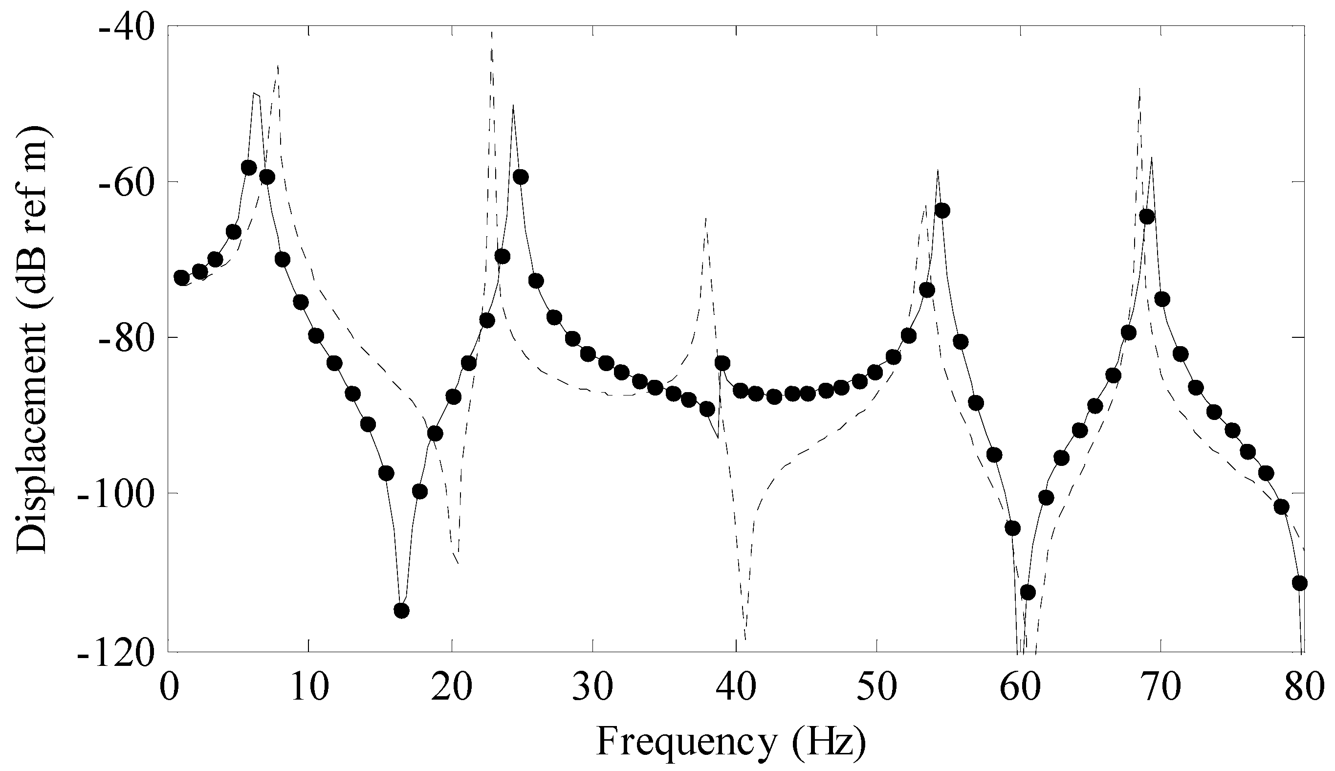
The integral from Equation (13) is identical to Equation (21). Figure 5 is a comparison of this series solution (solid line) to a previously derived analytical solution for a rod (circular markers) and a uniform area rod (dashed line). The modal solution was calculated using 25 terms. The previously derived analytical solution is given by

$$\widehat{U}(x)=\{\begin{array}{ll}{\widehat{U}}_L(x)=C_1{\mathrm{J}}_0\left[\kappa \left(\frac{bL}{2m}+x\right)\right]+C_2{\mathrm{Y}}_0\left[\kappa \left(\frac{bL}{2m}+x\right)\right]& 0\le x\le \frac{L}{2}\\ {\widehat{U}}_R(x)=C_3{\mathrm{J}}_0\left[\kappa \left(\frac{-2mL-bL}{2m}+x\right)\right]+C_4{\mathrm{Y}}_0\left[\kappa \left(\frac{-2mL-bL}{2m}+x\right)\right]& \frac{L}{2}\le x\le L,\end{array}$$

(44)

where the constants $C_1$, $C_2$, $C_3$ and $C_4$ are determined from the boundary conditions

$${\widehat{U}}_L(0)=0,$$

(45)

$${\widehat{U}}_L(L/2)-{\widehat{U}}_R(L/2)=0,$$

(46)

$$\frac{\mathrm{d}{\widehat{U}}_L(L/2)}{\mathrm{d}x}-\frac{\mathrm{d}{\widehat{U}}_R(L/2)}{\mathrm{d}x}=0$$

(47)

and

$$A(L)E\frac{\mathrm{d}{\widehat{U}}_R(L)}{\mathrm{d}x}=-F_0.$$

(48)

Note that this analytical solution method is valid for any cross-sectional area that can be represented by a Fourier series as the only change necessary for other shapes is a modification of the $c_q$ coefficients that comprise the area and derivative of area terms. The evaluation of the integrals in Equations (30)–(43) is unchanged for any other rod area and change of area represented by a Fourier series. Figure 6 is a plot of the convergence of the system versus number of summation terms and frequency. This convergence metric was calculated using Equation (26). The region in white is −40 dB (or lower) and this corresponds to a one percent (or less) normalized difference between the two solutions. Note that more terms are needed to achieve a one percent convergence compared to the first example problem. This is due to the added complexity of the shape of the rod for this example.

The third problem analyzed is a rod that has a variation in cross-sectional area proportional to a Bessel function, as shown in Figure 7. For this problem, the area is equal to

$$A(x)=2wb{\mathrm{J}}_0(mx)>0\forall x\in [0,L]$$

(49)

and the derivative of the area with respect to the longitudinal variable is

$$\frac{\mathrm{d}A(x)}{\mathrm{d}x}=-2wbm{\mathrm{J}}_1(mx).$$

(50)

In Equation (49) ${\mathrm{J}}_0$ denotes a zero order Bessel function of the first kind and in Equation (50) ${\mathrm{J}}_1$ denotes a first order Bessel function of the first kind. Closed form solutions to the integrals in Equations (10) and (11) do not exist, however, the problem can still be solved by numerically integrating these equations and using Equation (14) to calculate the wave propagation coefficients. Figure 8 is a comparison of this series solution (solid line) to a finite element solution for a rod (square markers) and a uniform area rod (dashed line). For the analytical model, a 51 point trapezoidal integration algorithm was used to compute the integrals for every value of p and n and the series solution was calculated using 25 terms. The finite element analysis is included for verification as a closed form solution does not exist for this geometry. It was created with the Abaqus FEA finite element program using linear elastic and steady-state direct analysis. The model used an eight node fully elastic continuum element with 100 elements and 804 nodes. Each element had a length of 0.03 m and this corresponds to approximately 38 elements per wave length at 80 Hz. The analytical model runs in 0.945 s while the finite element model takes about 90 s to compute, so the speed of the analytical model is almost two orders of magnitude faster than the finite element analysis. The above finite element time does not include building the mesh, which typically takes one to two hours. 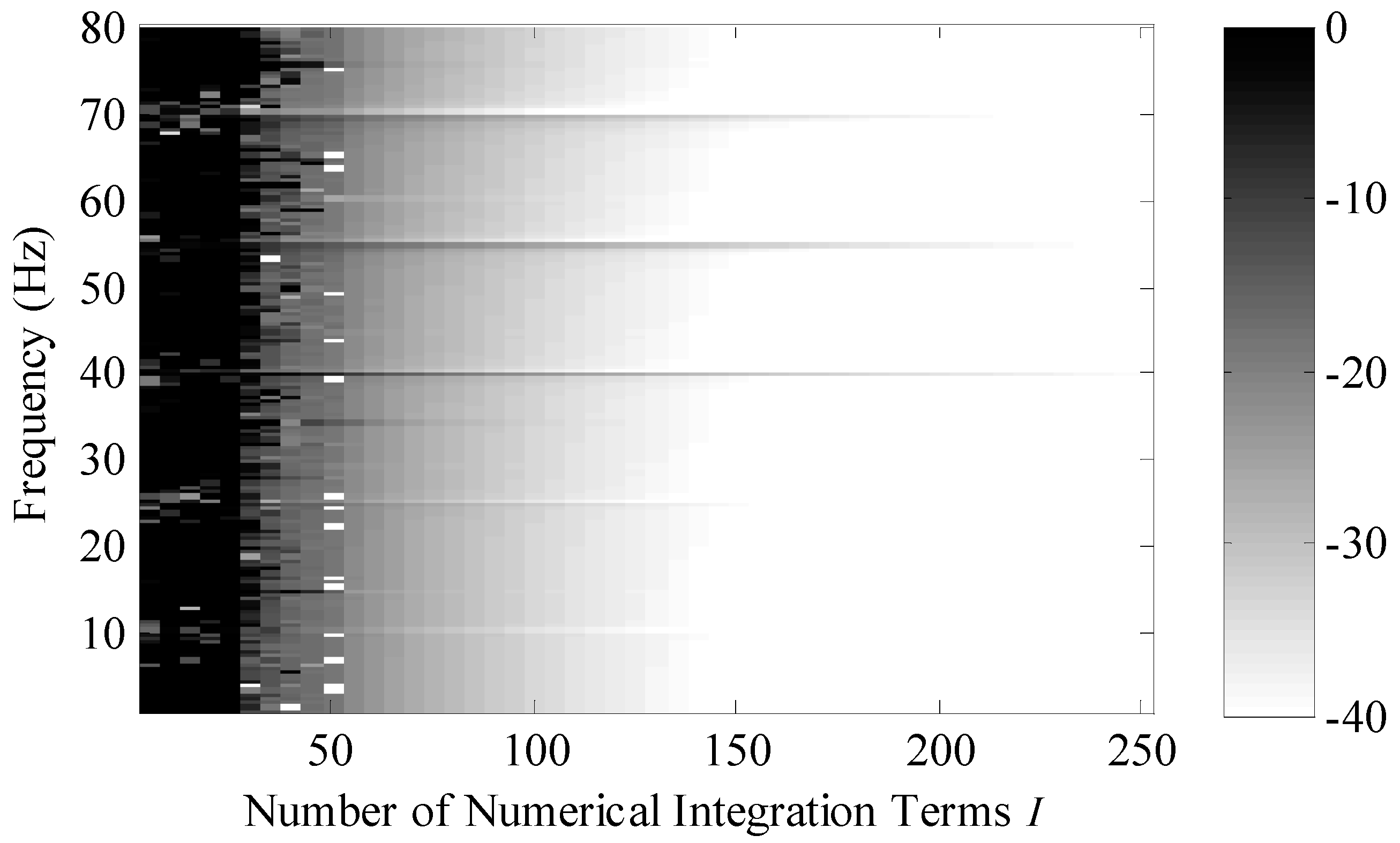Figure 9 is a plot of the convergence of the system versus number of integration points and frequency. This convergence metric was calculated using the Equation (26) where $\widehat{U}(x_j)$ is the series solution calculated using 100001 integration points and $U(x_j)$ is the series solution calculated using I integration points. The region in white is −40 dB (or lower) and this corresponds to a one percent (or less) normalized difference between the two solutions. Note that approximately 140 integration points are needed to make the two models converge and that this number is independent for the frequency range of the analysis presented here.

The fourth problem analyzed is a rod that has a variation in cross-sectional area proportional to the Gamma function, as shown in Figure 10. For this problem, the area is equal to

$$A(x)=2wb\mathsf{\Gamma }(mx+c)>0\forall x\in [0,L]$$

(51)

and the derivative of the area with respect to the longitudinal variable is

$$\frac{\mathrm{d}A(x)}{\mathrm{d}x}=2wbm\mathsf{\Gamma }(mx+c)\psi (mx+c).$$

(52)

In Equations (50) and (51) $\mathsf{\Gamma }$ denotes the Gamma function and in Equation (52) $\psi$ denotes the Psi (or Digamma) function. The variable c is used to avoid the infinite response of the Gamma function at x = 0 and is dimensionless. For this analysis, c is equal to 0.1. Similar to the last example problem, closed form solutions to the integrals in Equations (10) and (11) do not exist. The problem is solved by numerically integrating these equations and using Equation (14) to calculate the wave propagation coefficients. Figure 11 is a comparison of this series solution (solid line) to a uniform area rod (dashed line).

The second order differential equation is the governing equation for a large number of systems. Rods, membranes, tensioned strings, discrete particle dynamics, ocean acoustics and transonic flow are among the various problems that are modeled using a form of this equation. Generically, this equation can be written as

$$M(x)\frac{{\mathrm{d}}^{2}U(x)}{\mathrm{d}{x}^2}+N(x)\frac{\mathrm{d}U(x)}{\mathrm{d}x}+P(x)U(x)=F(x),$$

(53)

where $M(x)$, $N(x)$ and $P(x)$ are continuous functions that comprise the non-constant differential equation. A number of analytical solution sets have been generated with this equation when $M(x)$, $N(x)$ and $P(x)$ are of the same functional form. In general, when these functions have different analytical forms, closed-form solutions are unknown. The method derived here provides a semi-analytical solution to this class of problems. If the method developed above is applied to Equation (53), the result is

$$\mathbf{u}={\left[\mathbf{M}+\mathbf{N}+\mathbf{P}\right]}^{-1}\mathbf{f},$$

(54)

where

$$M_{p,n}={\displaystyle \underset{a}{\overset{b}{\int }}M(x)\frac{{\mathrm{d}}^2{\phi }_n(x)}{\mathrm{d}{x}^2}}{\phi }_p(x)\mathrm{d}x,$$

(55)

$$N_{p,n}={\displaystyle \underset{a}{\overset{b}{\int }}N(x)\frac{\mathrm{d}{\phi }_n(x)}{\mathrm{d}x}}{\phi }_p(x)\mathrm{d}x,$$

(56)

$$P_{p,n}={\displaystyle \underset{a}{\overset{b}{\int }}P(x){\phi }_n(x)}{\phi }_p(x)\mathrm{d}x,$$

(57)

$$u_{p,1}=U_p$$

(58)

and

$$f_{p,1}={\displaystyle \underset{a}{\overset{b}{\int }}F(x){\phi }_p(x)\mathrm{d}x}.$$

(59)

Note that if a is nonzero, then the eigenfunction has to be spatially shifted to account for this offset from the origin and the interval length L is equal to b − a.

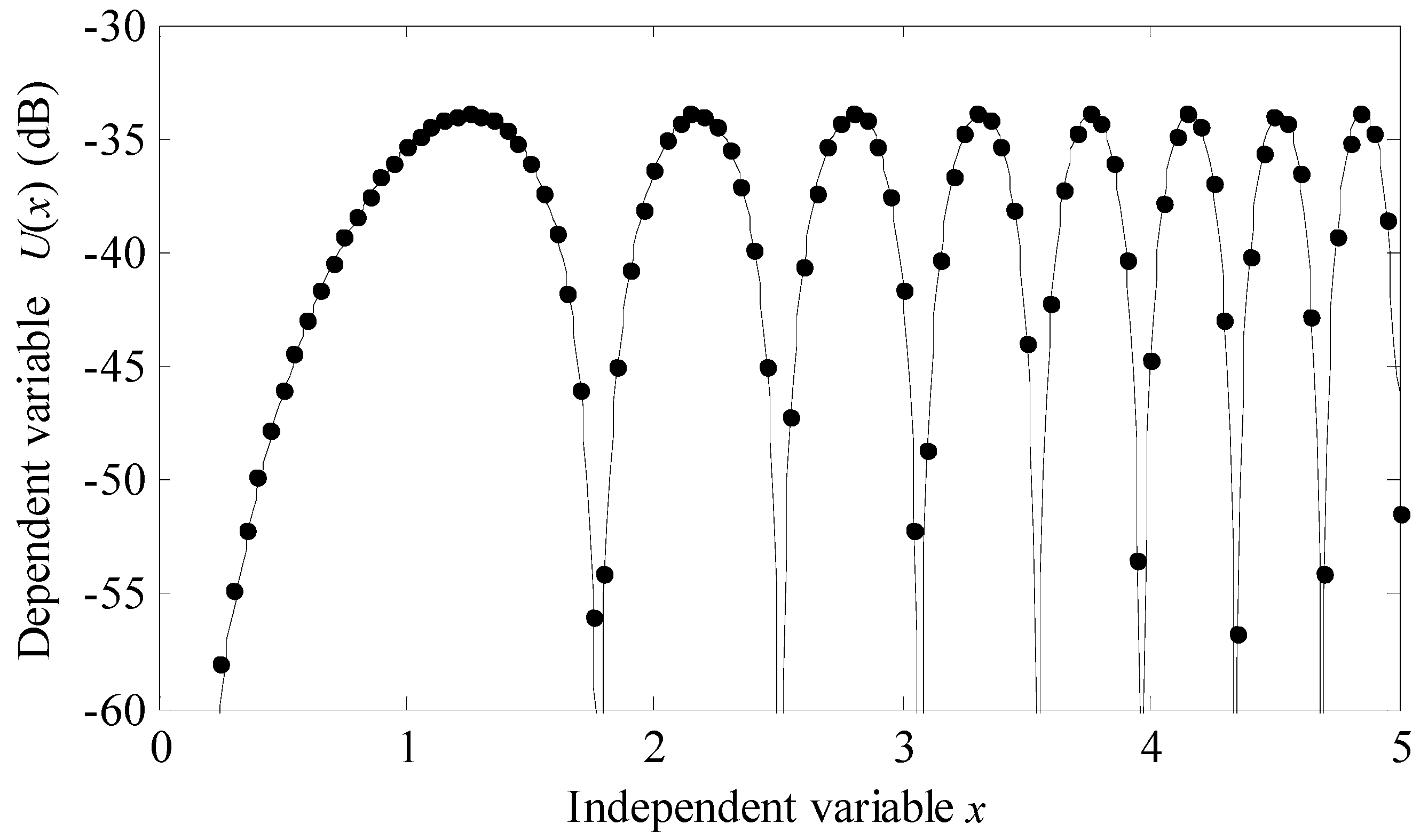
The fifth problem analyzed a differential equation of the form

$$x\frac{{\mathrm{d}}^{2}U(x)}{\mathrm{d}{x}^2}-\frac{\mathrm{d}U(x)}{\mathrm{d}x}+4x^{3}U(x)=\mathsf{\delta }(x-b),$$

(60)

with the boundary conditions of

$$U(a=0)=0$$

(61)

and

$$\frac{\mathrm{d}U(b=5)}{\mathrm{d}x}=0.$$

(62)

This problem was chosen because $M(x)~x$, $N(x)~x^0$ and $P(x)~x^3$, thus for this specific problem a closed form solution exists and is

$$U(x)=\frac{\sin (x^2)}{2b^2\cos (b^2)}.$$

(63)

Figure 12 is a comparison of the series solution (solid line) to the closed form solution (circular markers). This series solution was generated using 100 terms in the series expansion and 1001 integration points at every entry in the matrix equation.

4. Conclusions

This paper has shown that the eigenvalues and eigenfunctions of the rod with uniform area can be used to calculate a semi-analytical modal solution to the rod with a non-uniform area. Inserting these eigenfunctions with undetermined coefficients into the rod differential equation, a set of linear equations can be generated and solved to yield the displacement of the system at any location. Five example problems were computed and four of them were verified by a second solution method. This new work provides the framework to analyze any non-uniform area rod where the area can be represented as an analytical function. This method is extremely useful for cases where there is no known analytical solution and is much less time consuming than formulating a finite element analysis. Additionally, it was shown that any area change that can be represented with a Fourier series can be solved in matrix form with closed-form analytical expressions. The solution method can also be extended to any second order non-constant coefficient differential equation. Further work in this area should look to expand this solution method to fourth order beam and plate problems.