1. Introduction
The electromagnetic fields excited by a dipole source in a layered dissipative medium structure have been investigated widely because of their applications in Through-the-Earth communication, underwater communication, ground penetrating radar technology, and antenna design [
1,
2,
3,
4,
5,
6]. The developments in electromagnetic field propagation in layered medium structures have been analyzed by many investigators, including Wait [
7,
8,
9] and King [
7,
10,
11] who proposed the asymptotic methods, and the surface-impedance technique has been used for a two-layered region. Contour integrations and ranch cuts have been also used for the electromagnetic field in a layered region [
8,
9]. King et al. have obtained the complete formulas for electromagnetic fields excited by horizontal and vertical electric dipoles in two- and three-layered regions by using the proposed method in the recent studies. However, it is difficult to solve the arbitrary layered region problem. To overcome this drawback, Michalski et al. [
12] presented a compact formulation of the electric-type and magnetic-type dyadic Green’s functions for a plane-stratified, laterally unbounded multilayered structure, which is based on the tranmission-line network. Nikita et al. [
13] has presented a near-fielding radiating dipole antenna next to a three-layered lossy sphere close to a human head model. Moreover, the numerical results have been verified via a unified method of moments (MoM) model based on the electric field integral equation (EFIE) given by Khamas [
14]. These algorithms are suitable for analyzing the non-planar electromagnetic problem only when the structure is a concentric sphere, which limits their application in an arbitrary shaped non-planar layered region. Quintana et al. [
15] studied the electromagnetic field propagation characteristic of shallow water in detail, and the influence of seabed layer is also considered.
In most studies [
16,
17,
18,
19], surface integral equation (SIE)-based methods have been adopted in the numerical analysis of the scattering of arbitrary shaped objects and the scattering of objects buried in layered structure, but few of them focus on the electromagnetic fields excited by dipoles in arbitrary layered dissipative media. In this paper, an SIE-based method to study the electromagnetic fields excited by electric dipole submerged in arbitrary layered homogeneous dissipative media is proposed. The total electromagnetic fields in each layer with three source components including the excitation source itself, equivalent electric/magnetic surface currents at the top of the layer, and equivalent electric/magnetic surface currents at the bottom of the layer are derived in detail. Then, the formulation proposed for the interface of each layer is discretized by using the Galerkin’s method. After that, a matrix equation for a layered dissipative structure with a block tridiagonal matrix feature of a convenient solution is derived [
20]. Three application scenarios are constructed and computed to analyze the electromagnetic characteristics with the vertical and horizontal dipole buried in wide, practically important media including sea, wet and other dissipative materials. Finally, the numerical results are presented to discuss the difference of the proposed method in comparison with the Computer Simulation Technology (CST) Studio Suite.
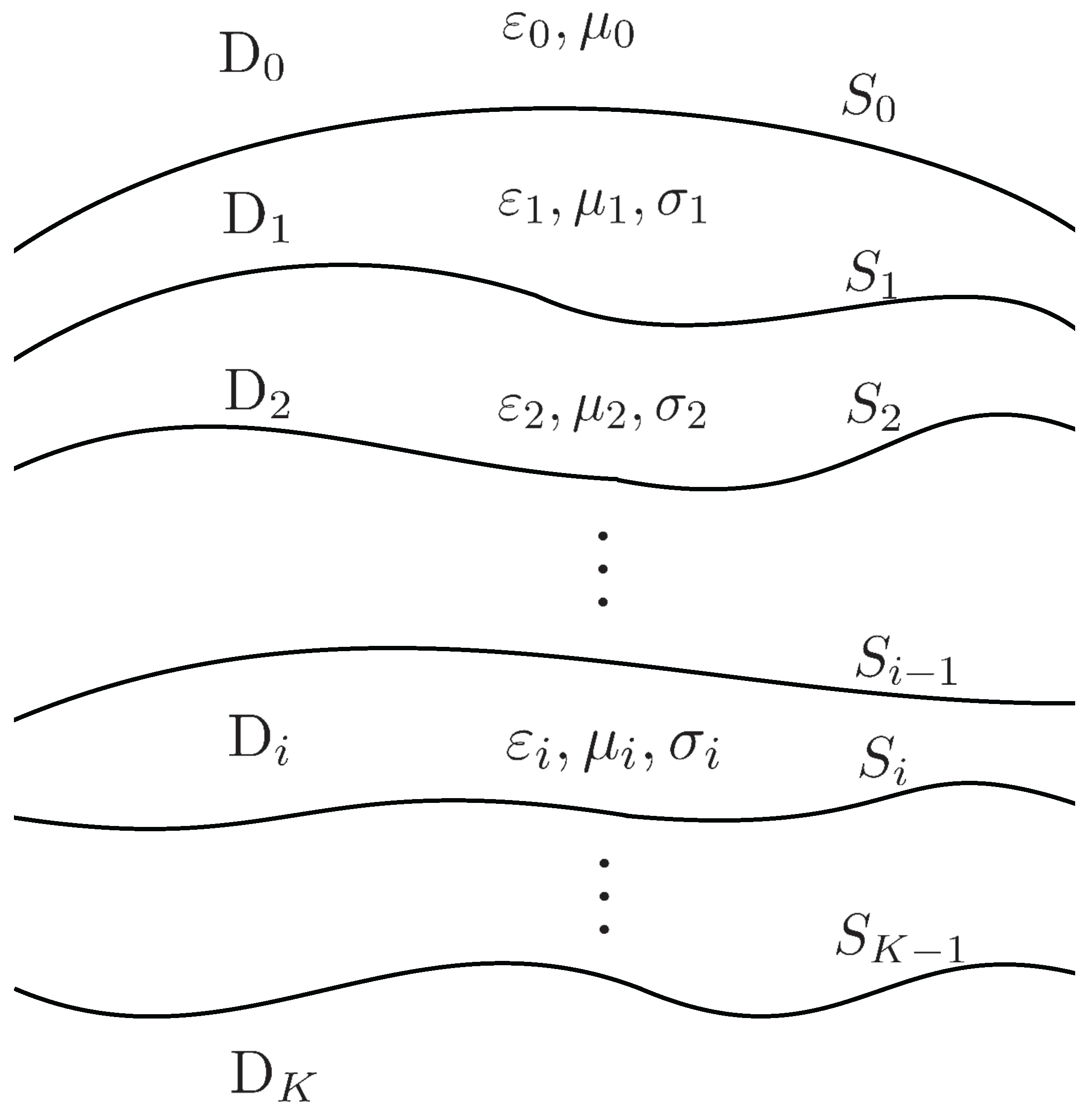
2. SIEs for Multilayered Dissipative Medium Structures
A non-planar
K-layered dissipative medium structure is illustrated in
Figure 1. Let the frequency of excitation sources in homogeneous medium be
. The electromagnetic constants at the
ith-layer are denoted by conductivity
, permittivity
, and permeability
, with complex wave number
and wave resistance
. Let
and
denote the top and bottom surfaces of
ith-layer medium of the region
, respectively, where
. In addition, there is no top surface on the half-space region
and no bottom surface beneath the half-space region
.
Let denote the incident fields in region , which can be excited by electric dipole antennas or magnetic dipole antennas. According to the equivalent principle, the total fields in region can be seen as a synergistic result of the incident fields , fields excited by the surface currents on , and fields excited by the surface currents on .
Hence, the total electric and magnetic fields at arbitrary point on surface
or
can be expressed as
The electric and magnetic surface currents on surface
in region
are defined as
and
, where
is the normal vector of
pointing to the inside of the region
. Because electric and magnetic currents on each interface shall be continuous across the boundary, the electric and magnetic surface currents on
are
in region
and
in region
. Based on the electric and magnetic field integral equations [
17,
21,
22], the induced electric and magnetic fields
and
in region
excited by surface current
and
can be written as
The linear operator
and
can be defined as
where
is the surface divergence of a vector field. The Green’s function in homogeneous isotropic infinite space is given by
where
is the wave number of region
,
is the field point and
is the source point.
According to the definition of the surface currents [
19], for a field point
in region
, the tangential component of electric and magnetic fields can be written as Equations (
7)–(
10). The left-hand side are induction fields and right-hand side can be expressed in terms of incident fields.
Similarly, for
in
,
For
, the linear operator
K in (
5) needs to be split into two parts [
22,
23,
24,
25]:
where
denotes the Cauchy’s principal value integration with
for smooth surface, and
is the outward directed normal vector of the integral surface. By substituting Equation (
11) into Equations (
7)–(
10), we get the electromagnetic fields on the surface in region
,
Similarly, we can also calculate the electromagnetic fields on surface
in region
,
Combining Equations (
13) and (
16), electric field on surface
can be written as,
The magnetic field on surface
is obtained by combining Equations (
15) and (
17),
3. Discretization
For numerical solutions of equivalent electric and magnetic currents on the media interfaces, the Galerkin’s method and the Rao–Wilton–Glisson (RWG) basis functions [
16,
26] are utilized to discretize the continuous formulations Equations (
18) and (
19) [
27]. The media interface of each layer is discretized into planar triangular elements, with
which is defined as the
nth triangular element on surface
,
and
.
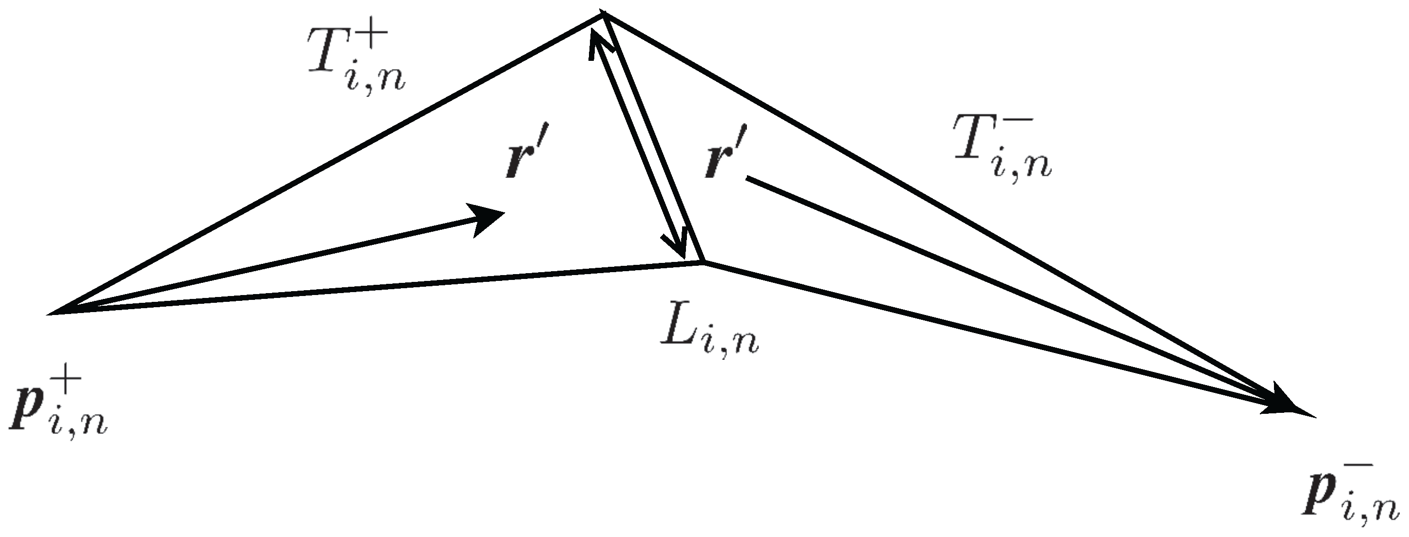
The RWG basis function
assigned to a pair of triangular elements on surface
is defined as:
where
and
are the vertex of triangular elements
and
, which share a common edge of length
[
18].
and
are the areas of triangular elements
and
, respectively. Spatial distribution of RWG functions are shown in
Figure 2.
The unknown surface current distribution
and
on surface
are replaced by an expansion in the basis in numerical computations:
where
and
are the
nth complex expansion coefficients of
and
. By substituting (
21) into (
18) and (
19), and testing them with RWG basis, the matrix equation for media interface
can be written as
where,
The submatrix in the matrix equation can be expressed as:
The basis
,
in medium
is operated by the linear operator
L and
K:
For
, the electric and magnetic excitation source matrix in
can be expressed as:
According to Equation (
22), the matrix equation for all surfaces with block tridiagonal matrix equation is derived as follows:
Equation (
39) is the relation between the surface current, impedance matrix and incidence fields in
K-layered dissipative medium structures. The impedance matrix is a square matrix with the number of elements equal to
, with
non-zero data in the impedance matrix. Both the number of unknown surface current coefficients and excitation source matrix are
. Therefore, the surface current coefficients can be obtained by solving the matrix equation.
4. Numerical Examples
In this section, three experiments are constructed to analyze the performance of the proposed method with the vertical or horizontal dipole buried in media including sea, wet and other dissipative materials. The algorithm is implemented by MATLAB 2011b on a computer with CPU i3-4030U working at 1.9 GHz with 4 GB RAM and a Windows 10 operating system. The Low Frequency (LF) Domain Solver of CST Studio Suite in the same computer is used to simulate the models for comparison.
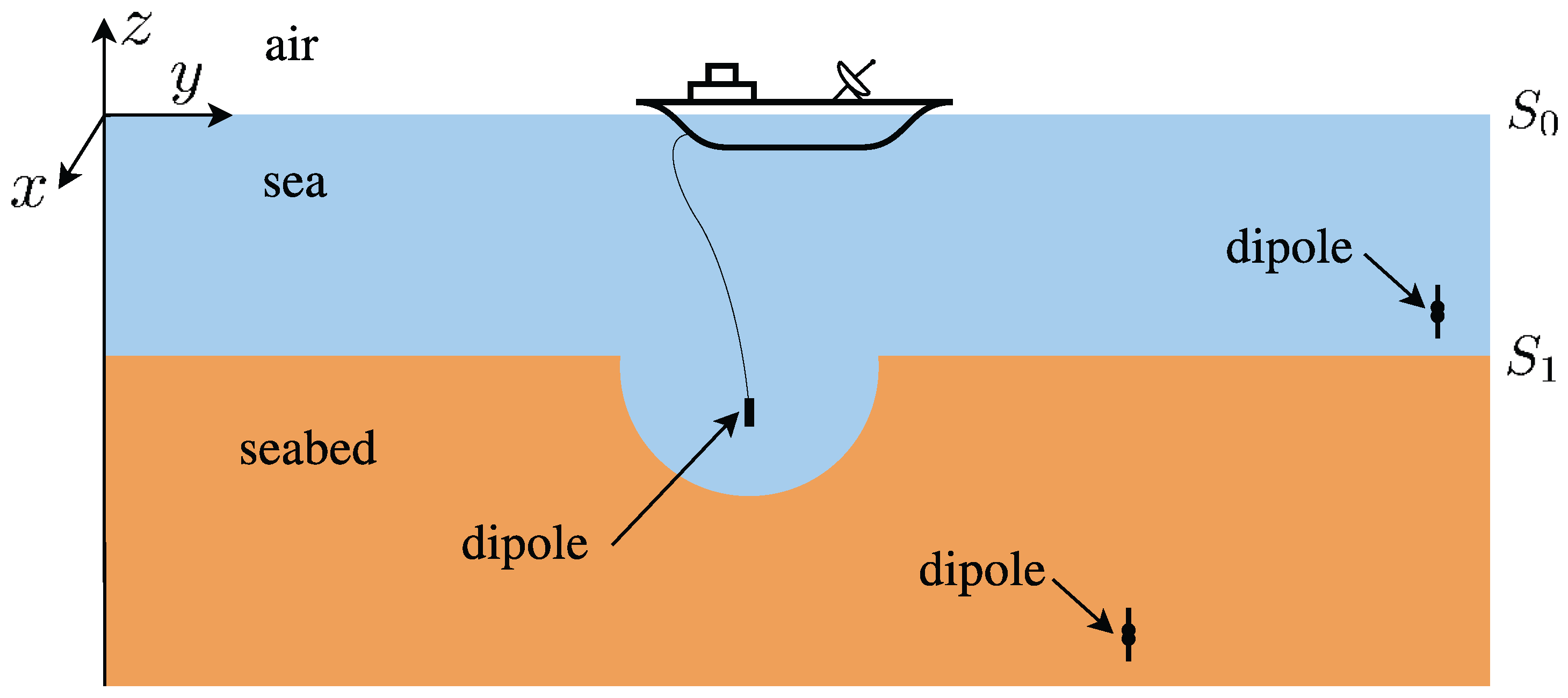
We first consider a non-planar air–sea–seabed structure with a hemispherical depression at the seabed shown in
Figure 3 for the application that the naval vessel receives signals from the transmitter burried in the seabed. The air permittivity and permeability are
, respectively, which are the same as vacuum. Generally, the conductivity of the sea is
, and the permittivity and permeability of the sea are
and
, respectively. Conductivity of the seabed is
, with permittivity
and permeability
. Media interface
and
are both circular with radius
, located at plane
and
, respectively. The hemispherical depression is set at point
with radius
. A vertical electric dipole excitation source is located at point
, with dipole moment
and the frequency is 100 Hz. In order to reduce the mesh amount, we refine the mesh in the source areas and other part is sparse. The number of triangles on the air–sea interface
and the sea–seabed interface
are 856 and 1528. As a result, 7088 unknowns are generated. In numerical calculations, the processor takes
s and
GB to solve the matrix equation. However, the calculation of the same model with
unknowns using CST takes 156 s and
GB of memory.
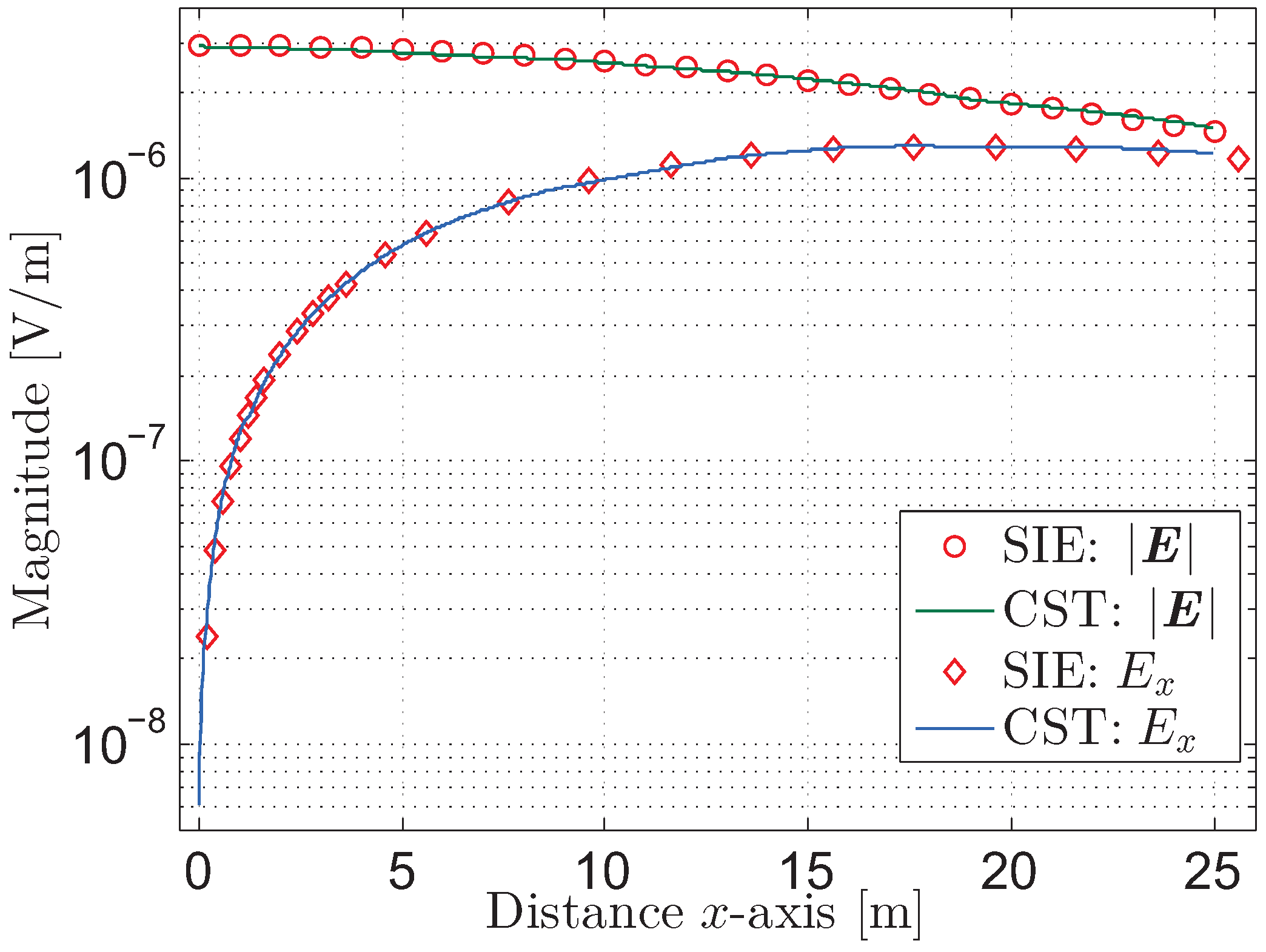
Figure 4 shows the
x-direction electric field and the total electric field at point
,
. The results calculated by CST are also plotted in
Figure 4 for comparison. These results show clearly that the numerical results calculated by the proposed method are close to the results computed by CST, with most errors within a range of
. However, from the results listed in
Table 1, it can be observed that there are relatively large errors in the first and last column, which are larger than
. As the electric field in
close to
z-axis is a minimum value, non-uniform discretized mesh can introduce a relatively large error to the first column in numerical calculations. The sparse mesh far from source also causes large error in the last column. It can be also observed from the results in
Table 2 that most of the results are within the error range of
. However, there is relatively large error when field point is in the sparse mesh area. The comparisons indicate that the proposed method provides good performance in solving time and high accuracy results for the electric dipole in the two-layered dissipative structure.
For the second example, we consider the air–rock–earth–mine layered structure shown in
Figure 5. It can be used in Through-The-Earth communication for mines, where communication devices communicate with other nodes by using horizontal electric dipoles located in the earth layer. The frequency of excitation source is 10 kHz. The conductivity of the rock layer is
, and the permittivity and permeability of the rock are
and
, respectively. Conductivity of the earth layer is
, with permittivity
and permeability
. The conductivity of the mine layer is
, and the permittivity and permeability of the mine are
and
, respectively. Media interfaces
,
and
are circular of radius
. Media interfaces
,
and
are located at plane
,
and
. The
x-directional horizontal electric dipole with dipole moment
is located at
.
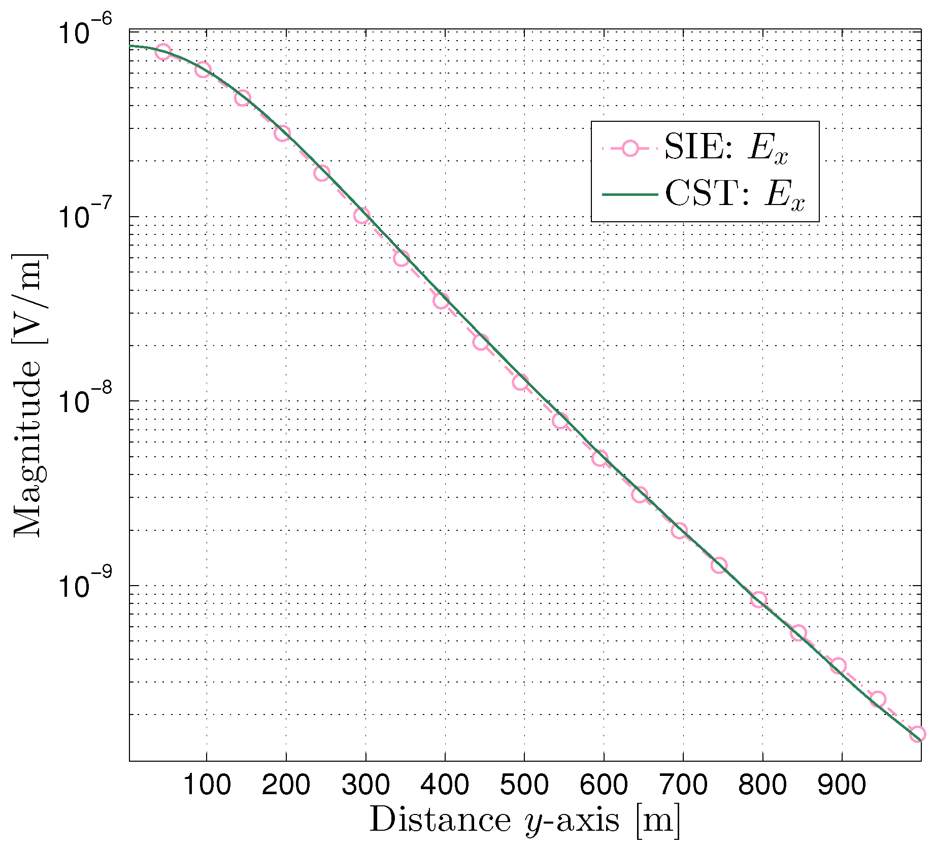
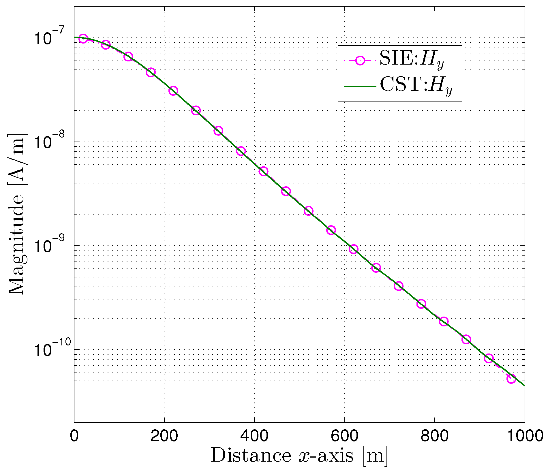
The
x-component electric field propagation at point
,
is plotted in
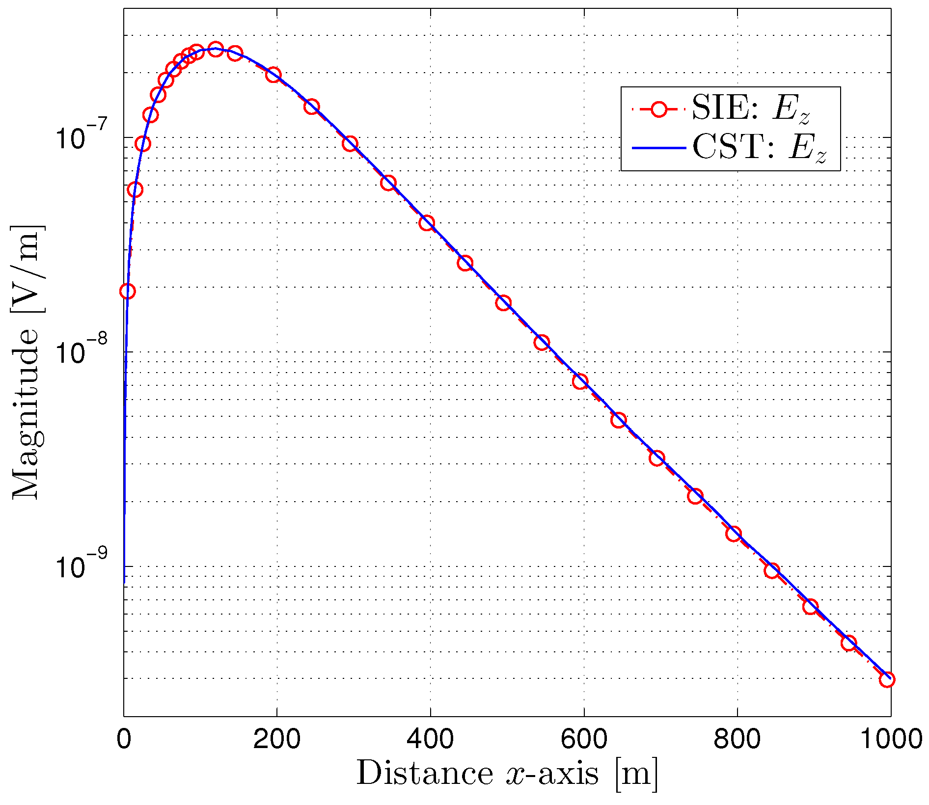
Figure 6. The
z-component electric field propagation and the
y-component magnetic field propagation at point
,
are plotted in
Figure 7 and
Figure 8, respectively. We can notice that the numerical results calculated by the proposed method are close to the results computed by CST. It can be observed from
Table 3,
Table 4 and
Table 5 that most of the numerical results are within the error range
. The mesh is sparse at the boundary area, which results in relatively large deviation when the test point gets closer to the boundary, and the magnetic field results are more accurate than electric field results.
Each of the interfaces , and is meshed into 710 triangle patches, resulting in 6288 unknowns. It takes s and GB to solve the matrix equation by the use of the proposed method. However, the calculation of the same model with unknowns using CST takes 55 s and GB memory.
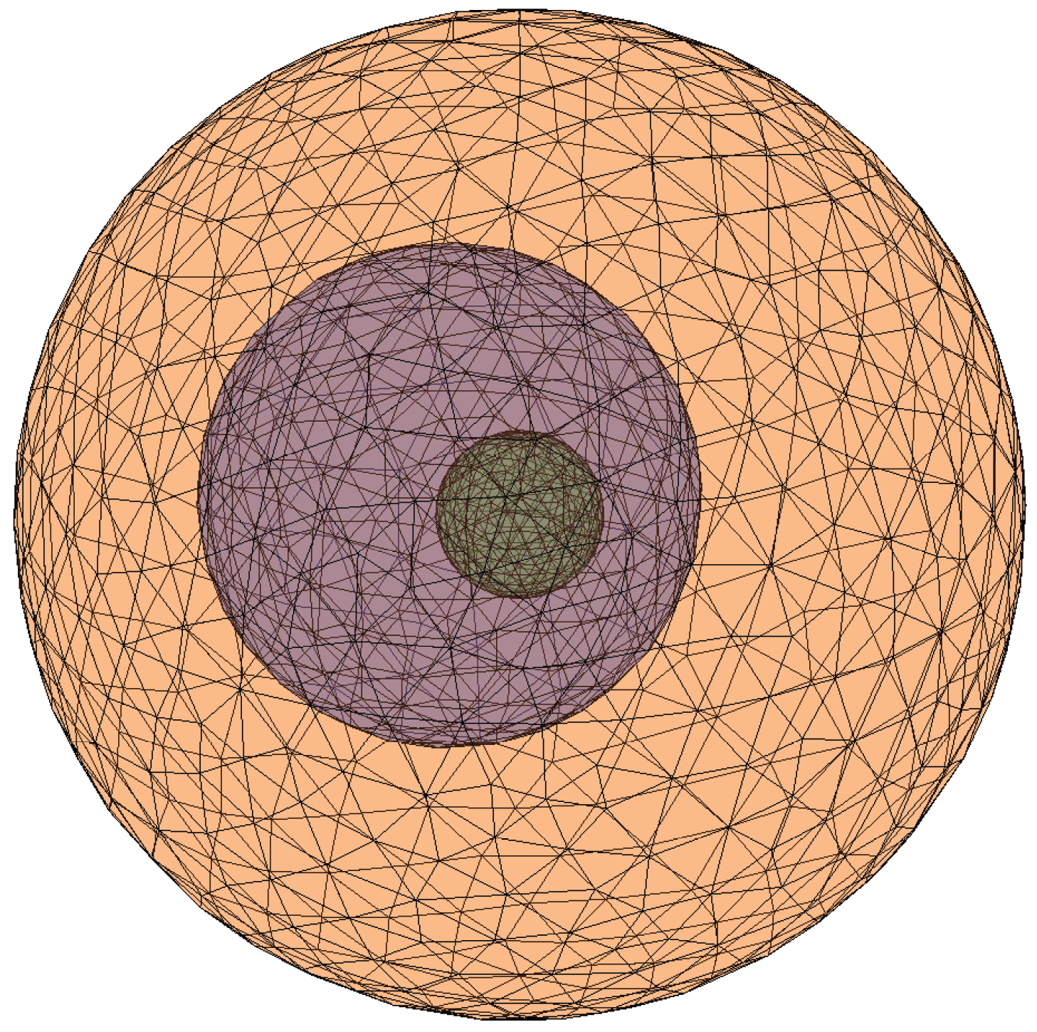
The proposed method is used to simulate the electromagnetic fields excited by horizontal electric dipole in a dissipative sphere, which is a closed structure coated by layered materials and is shown in
Figure 9. The external sphere is located at origin and has a radius of 6 m with conductivity
, permittivity
and permeability
. The radius of the middle sphere is 3 m with conductivity
, permittivity
and permeability
, which is located at point
. The internal sphere is located at origin and has a radius of 1 m, where the conductivity is
, permittivity is
, and permeability is
. A horizontal electric dipole excitation source is located at origin with dipole moment of
along
x-axis, and the frequency is 1 MHz. After discretization, the numbers of triangles on the external sphere
, the middle sphere
and the internal sphere
are 1204, 604 and 626, respectively. As a result, 7302 unknowns are generated. It takes
s and
GB of memory to solve the matrix equation in numerical calculations. Compared with the proposed method, the calculation of the same model with
unknowns using CST takes 150 s and
GB of memory, which shows that the proposed method has a good performance in solving time and storage space.
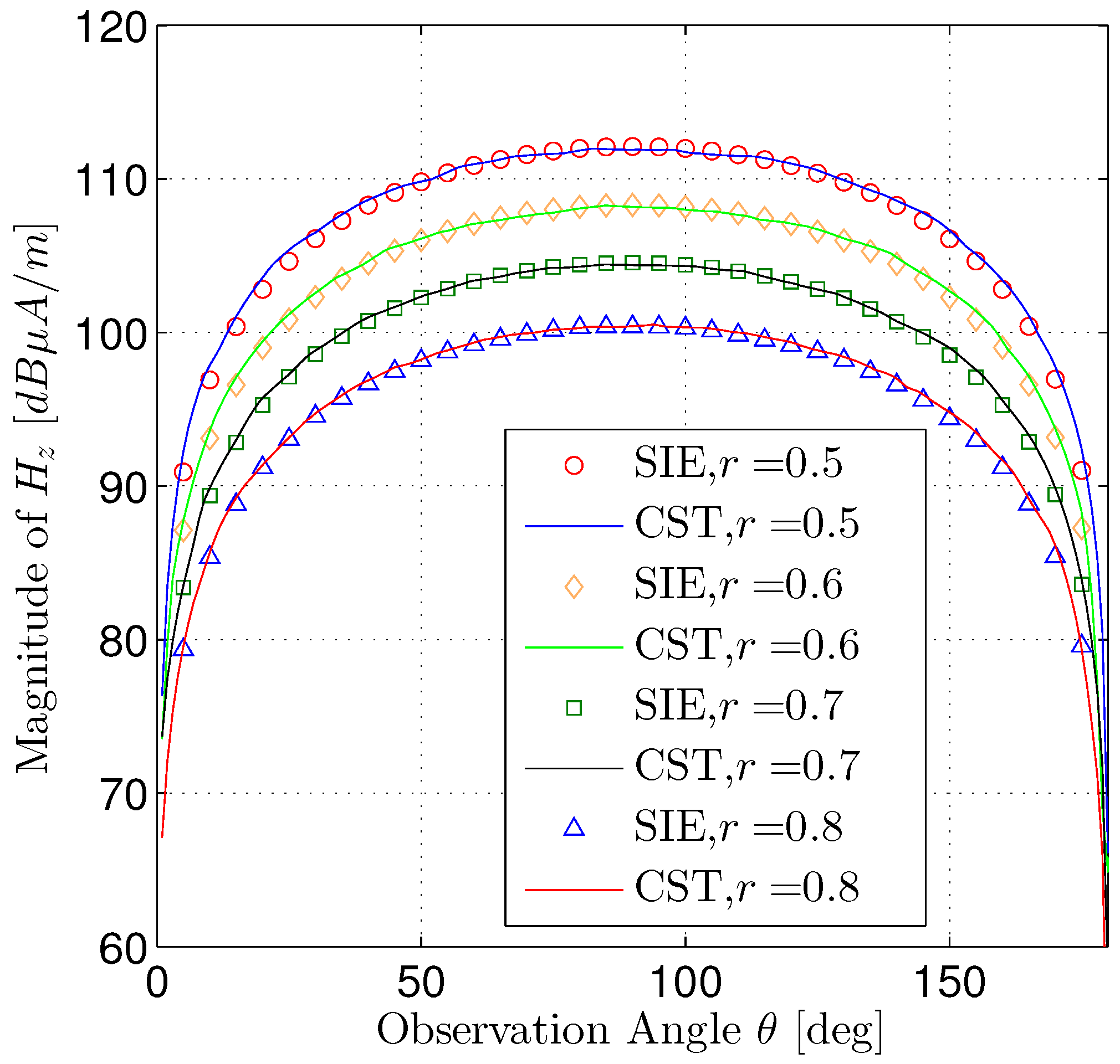
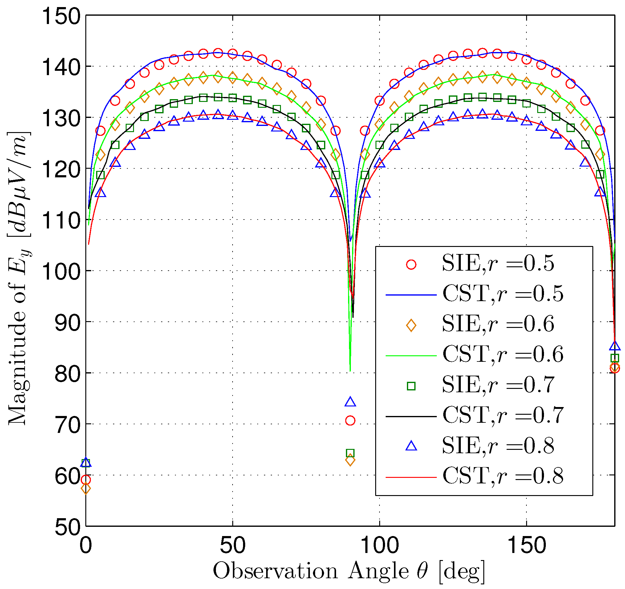
Figure 10 shows the near magnetic field component
as a function of the observation angle in plane
, and
Figure 11 illustrates the near electric field component
, which are compared with CST. We can observe that the numerical results obtained from the proposed method are in good agreement with the results obtained by CST.
Figure 12 gives the root-mean-square (RMS) error of different observation radius. The Root-mean-square (RMS) error is given by [
28]:
where
is the calculated quantity and
refers to the corresponding CST result. We can see that the
RMS error is smaller than that of
of each observation radius. It indicates that the proposed method has a better performance in solving magnetic field than solving electric field. In the CST model, the excitation source is a quasi-ideal horizontal electric dipole. As a result, the comparison model is different from our simulation model, and the RMS error seems to be higher when the observation point is close to the source. When the observation radius are larger than
m, the numerical results are still in good agreement with the comparison model with RMS error of less than
for magnetic fields and
for electric fields.


