Performance Analysis and Design Strategy for a Second-Order, Fixed-Gain, Position-Velocity-Measured (α-β-η-θ) Tracking Filter

Featured Application

Design and evaluation of monitoring systems in intelligent vehicles, robots, and so on.

Abstract

We present a strategy for designing an $\alpha$-$\beta$-$\eta$-$\theta$ filter, a fixed-gain moving-object tracking filter using position and velocity measurements. First, performance indices and stability conditions for the filter are analytically derived. Then, an optimal gain design strategy using these results is proposed and its relationship to the position-velocity-measured (PVM) Kalman filter is shown. Numerical analyses demonstrate the effectiveness of the proposed strategy, as well as a performance improvement over the traditional position-only-measured $\alpha$-$\beta$ filter. Moreover, we apply an $\alpha$-$\beta$-$\eta$-$\theta$ filter designed using this strategy to ultra-wideband Doppler radar tracking in numerical simulations. We verify that the proposed strategy can easily design the gains for an $\alpha$-$\beta$-$\eta$-$\theta$ filter based on the performance of the ultra-wideband Doppler radar and a rough approximation of the target’s acceleration. Moreover, its effectiveness in predicting the steady state performance in designing the position-velocity-measured Kalman filter is also demonstrated.

1. Introduction

Monitoring systems for robots and intelligent vehicles that employ remote sensors, such as cameras and radar, require the tracking of moving objects. Adaptive tracking techniques such as Kalman and extended Kalman filters [1,2,3,4,5] and particle filters [6,7] are commonly used for this purpose because of their accuracy. An alternative option is fixed-gain tracking filters, which have also been studied and used extensively for two reasons [8,9,10,11,12]:

• Simple implementation and low computational overhead: Optimal gain calculation is not required in the fixed-gain filters. Thus, the number of matrix operations is small compared with the Kalman filter and its variants [11].
• Applicability to the analytical evaluation of the Kalman filter: Fixed-gain filters are also useful for analytical evaluations of the Kalman filter because they can be characterized as steady state Kalman filters [12].

For these reasons, fixed gain filters are still being widely used in applications that strongly require real-time capability and simple implementation, such as tracking in ultrasonography in medicine [13], motor position control [14], human fall detection [15] and vehicular radar [16]. Additionally, the analysis of the Kalman filters assuming the steady state (fixed gain) is conducted to predict their tracking performance in the filter design process. The simplest second-order fixed-gain tracking filter is known as an $\alpha$-$\beta$ filter, which have been deployed in various tracking systems [12,17,18,19,20,21,22]. The design of the $\alpha$-$\beta$ filter has been discussed based on an efficient design parameter known as the tracking index [10,12,22].

However, $\alpha$-$\beta$ filters only consider position measurements and hence cannot make full use of modern sensors that can also measure velocity, such as ultra-wideband (UWB) Doppler radars, which have recently come into use [23,24,25]. In the near-field, these radars can achieve accurate sensing of moving objects, such as humans and cars. In [23,24], position and velocity estimates for pedestrians were achieved with centimeter and cm/s accuracy, respectively (see [25] for hardware implementation). Moreover, sensor fusion based on the Internet of Things technology also enables the simultaneous measurement of position and velocity possible (e.g., sensor data fusion based on the communication between radars and speedometers embedded in targets). Consequently, tracking filters for such systems have become an important area of research [26,27,28,29]. However, almost all conventional position-velocity-measured (PVM) trackers have been based on Kalman or particle filtering, whereas fixed-gain PVM filters have not seen wide use. This is because the computational performance is sufficient to drive PVM Kalman/particle filters in many applications. Additionally, the empirical design of these filters without steady state analyses can realize tolerable tracking performance. However, reiterating, fixed gain filter techniques are still important for various applications and analytical performance evaluation of tracking systems to find better parameter settings.

To address the above problem, we have proposed third-order fixed-gain ($\alpha$-$\beta$-$\gamma$) PVM filters and have verified their performance [11]. However, a simpler second-order tracker such as an $\alpha$-$\beta$ filter is often required when the number of components and/or the size of hardware is quite limited and the complexity of target motion is predicted to be relatively small (i.e., a constant velocity model assuming a second-order tracker is sufficient). To this end, we also have investigated the fundamental properties of a PVM $\alpha$-$\beta$ filter [30]. However, this filter assumes an unrealistic assumption; specifically, correlated errors of position and velocity do not exist in the filtering process. As a realistic second-order fixed gain filter, Sudano [31] proposed a fixed-gain, position-velocity-measured, second-order tracking filter, described as an $\alpha$-$\beta$-$\eta$-$\theta$ filter. This filter corresponds to the $\alpha$-$\beta$ filter in position-only-measured tracking problem, and the relationship between $\alpha$-$\beta$-$\eta$-$\theta$ and the PVM Kalman filters is similar to that between the $\alpha$-$\beta$ and Kalman filters. Therefore, we believe that although the $\alpha$-$\beta$-$\eta$-$\theta$ filter is underutilized at present, this filter will be widely used like the $\alpha$-$\beta$ filter after the spread of PVM systems such as the UWB Doppler radar. Thus, clarifying the analytical properties and design strategy of the $\alpha$-$\beta$-$\eta$-$\theta$ filter is important for tracking technology in the near future. Although Sudano investigated the relationship of this filter with the PVM Kalman filter using a random-acceleration model based on the tracking indices, he did not discuss their performance or any design strategies. In addition, although Crouse [8] described a general solution for optimal fixed-gain trackers with steady state Kalman gains, he too did not discuss filter performance or a design strategy.

In this paper, a gain design strategy to compose an optimal $\alpha$-$\beta$-$\eta$-$\theta$ filter is proposed, and efficient performance indices are derived. The strategy is based on the method presented in [4] for Kalman filters, which optimizes an analytical performance index for the tracking filter. The proposed strategy provides the easy design of filter gains and accurate tracking of the $\alpha$-$\beta$-$\eta$-$\theta$ filter compared with the conventional empirical design methods. Furthermore, another important objective of this paper is to demonstrate, using numerical simulations, the effectiveness of the $\alpha$-$\beta$-$\eta$-$\theta$ filter obtained with the proposed strategy for a realistic UWB Doppler radar application. In this application, we show its effectiveness in the design of the PVM Kalman filter that has better steady state performance.

The remainder of this paper is organized as follows: Section 2 defines the tracking problem dealt with in this paper. Section 3 reviews the $\alpha$-$\beta$-$\eta$-$\theta$ filter of Sudano [31]. Its definition, relationship to conventional filters and design problems are described. Section 4 analytically derives the filter’s performance indices and stability conditions for an appropriate gain design. Section 5 proposes our design strategy and explores its relationship to the Kalman filter. Section 6 analyzes the performance of $\alpha$-$\beta$-$\eta$-$\theta$ filters designed with this strategy and compares it with the conventional filters. Section 7 presents a numerical application to realistic UWB Doppler radar tracking, and Section 8 offers concluding remarks.

2. Definitions of Problem and Symbols

This paper mainly considers the one-dimensional second-order moving object tracking filter assuming that only position and velocity measurements are considered. For the one-dimensional problem, only tracking along the x-axis is considered. Note that for the performance evaluation, assuming the realistic situation presented in Section 7, an actual two-dimensional tracking in the x-y plane is considered, and the one-dimensional tracking filter being considered is implemented for each axis in this simulation.

The inputs of the filter are measured target position $x_{\mathrm{o}}$ and velocity $v_{\mathrm{o}}$. This assumes that the observed data are both position and velocity. Note that many conventional studies on the tracking system adopt a position-only analysis, whereas assuming position/velocity measurements is one of the features of our study. The errors in $x_{\mathrm{o}}$ and $v_{\mathrm{o}}$ conform to white Gaussian noise, and their correlations are not considered for simplicity. We assume that the variance of the position measurement errors $B_{\mathrm{x}}$ and that of the velocity measurement errors $B_{\mathrm{v}}$ are known.

The outputs are predicted target position $x_{\mathrm{p}}$ and velocity $v_{\mathrm{p}}$ and smoothed (estimated) target position $x_{\mathrm{s}}$ and velocity $v_{\mathrm{s}}$. The focus of this paper is the optimization of the steady state accuracy in $x_{\mathrm{p}}$. To achieve this, the inputs $x_{\mathrm{o}}$ and $v_{\mathrm{o}}$ are filtered by some gains. This study assumes that these gains are unknown parameters that we must design. Thus, the purpose of this paper is the design of the tracking filter gains that minimizes the errors in the predicted target position.

The detailed definitions and explanations of the tracking filters and their design methodology that we focus on are presented in the rest of this paper.

Table 1. List of symbols.

Variables	Description	Unit
T	Sampling interval	(s)
k	Discrete sampling index	Dimensionless
${\left(\right)}_{,k}$	Parameter at index k
$x_{\mathrm{p}}$	Predicted position	(m)
$v_{\mathrm{p}}$	Predicted velocity	(m/s)
$x_{\mathrm{s}}$	Smoothed (estimated) position	(m)
$v_{\mathrm{s}}$	Smoothed (estimated) velocity	(m/s)
$x_{\mathrm{o}}$	Observed (measured) position	(m)
$v_{\mathrm{o}}$	Observed (measured) velocity	(m/s)
$\alpha$	Filter gain for $x_{\mathrm{s}}$ with respect to $x_{\mathrm{o}}$	Dimensionless
$\beta$	Filter gain for $v_{\mathrm{s}}$ with respect to $x_{\mathrm{o}}$	Dimensionless
$\eta$	Filter gain for $x_{\mathrm{s}}$ with respect to $v_{\mathrm{o}}$	Dimensionless
$\theta$	Filter gain for $v_{\mathrm{s}}$ with respect to $v_{\mathrm{o}}$	Dimensionless
$\widetilde{\left(\right)}$	Forecasts
$\widehat{\left(\right)}$	Estimates
${\left(\right)}^{\mathrm{T}}$	Transpose of matrix
${\left(\right)}^{-1}$	Inversion of matrix
$\mathit{x}$	State vector of target composed of position and velocity
$\mathit{z}$	Measurement vector
$\mathit{F}$	Transition matrix from k to $k+1$
$\mathit{P}$	Error covariance matrix with respect to $x$
$\mathit{Q}$	Covariance matrix of process noise
$\mathit{K}$	Kalman gain matrix
$\mathit{B}$	Covariance matrix of measurement noise
$B_{\mathrm{x}}$	Error variance of $x_{\mathrm{o}}$	(m${}^2$)
$B_{\mathrm{v}}$	Error variance of $v_{\mathrm{o}}$	(m${}^2$/s${}^2$)
${\mathit{Q}}_{\mathrm{ra}}$	Process noise matrix in random-acceleration (RA) model
q	Variance of random-acceleration (RA) process noise	(m${}^2$/s${}^4$)
$R_{\mathrm{xv}}$	Ratio of $B_{\mathrm{x}}$ to $T^2{B}_{\mathrm{v}}$	Dimensionless
E$\left(\right)$	Mean with respect to k
${\sigma }_{\mathrm{p}}^2$	Smoothing performance index	(m${}^2$)
$e_{\mathrm{fin}}$	Tracking performance index	(m)
$a_{\mathrm{c}}$	Acceleration assumed in the derivation of $e_{\mathrm{fin}}$	(m/s${}^2$)
${ϵ}_{\mathrm{rms}}$	Root-mean-square (RMS) index	(m)
$\mu$	Evaluating function in the proposed gain design strategy	Dimensionless
$a_{\mathrm{D}}$	Design parameter for the proposed strategy	Dimensionless
${\mathit{Q}}_{\mathrm{gen}}$	Arbitrary process noise matrix
a	(1,1) element of ${\mathit{Q}}_{\mathrm{gen}}$	(m${}^2$)
b	(1,2) (or (2,1)) element of ${\mathit{Q}}_{\mathrm{gen}}$	(m${}^2$/s)
c	(2,2) element of ${\mathit{Q}}_{\mathrm{gen}}$	(m${}^2$/s${}^2$)
$ϵ$	RMS prediction error of Monte Carlo simulations	(m)

lists the symbols used in this paper. Furthermore, each symbol is defined at its first appearance.

3. The $\alpha$-$\beta$-$\eta$-$\theta$ Filter

3.1. Definition

The $\alpha$-$\beta$-$\eta$-$\theta$ filter proposed by Sudano [31] is a second-order fixed-gain PVM tracker. It can be considered to be an extension of the $\alpha$-$\beta$ filter, which uses position measurements only. The $\alpha$-$\beta$-$\eta$-$\theta$ filter iterates prediction and smoothing (update) processes. The prediction process is conducted under the assumption that the target’s velocity is constant over the sampling interval and yields a position prediction:

$$\begin{array}{cc}\hfill x_{\mathrm{p},k}& =x_{\mathrm{s},k-1}+T{v}_{\mathrm{s},k-1},\hfill \end{array}$$

(1)

$$\begin{array}{cc}\hfill v_{\mathrm{p},k}& =v_{\mathrm{s},k-1},\hfill \end{array}$$

(2)

where $x_{\mathrm{s},k}$ is the smoothed target position at time $kT$, T is the sampling interval, $x_{\mathrm{p},k}$ is the predicted position, $v_{\mathrm{s},k}$ is the smoothed velocity and $v_{\mathrm{p},k}$ is the predicted velocity. The smoothing process is defined as in [31]:

$$\begin{array}{cc}\hfill x_{\mathrm{s},k}& =x_{\mathrm{p},k}+\alpha (x_{\mathrm{o},k}-x_{\mathrm{p},k})+T\eta (v_{\mathrm{o},k}-v_{\mathrm{p},k}),\hfill \end{array}$$

(3)

$$\begin{array}{cc}\hfill v_{\mathrm{s},k}& =v_{\mathrm{p},k}+(\beta /T)(x_{\mathrm{o},k}-x_{\mathrm{p},k})+\theta (v_{\mathrm{o},k}-v_{\mathrm{p},k}),\hfill \end{array}$$

(4)

where $x_{\mathrm{o},k}$ is the measured position, $v_{\mathrm{o},k}$ the measured velocity and $\alpha$, $\beta$, $\eta$ and $\theta$ are fixed filter gains that we must design.

3.2. The $\alpha$-$\beta$ Filter

The $\alpha$-$\beta$ filter is well known and popular in tracking because of its simplicity and utility in real-time applications. Its prediction steps are the same as for the $\alpha$-$\beta$-$\eta$-$\theta$ filter. The smoothing process is defined as in [10]:

$$\begin{array}{cc}\hfill x_{\mathrm{s},k}& =x_{\mathrm{p},k}+\alpha (x_{\mathrm{o},k}-x_{\mathrm{p},k}),\hfill \end{array}$$

(5)

$$\begin{array}{cc}\hfill v_{\mathrm{s},k}& =v_{\mathrm{p},k}+(\beta /T)(x_{\mathrm{o},k}-x_{\mathrm{p},k}).\hfill \end{array}$$

(6)

When $\eta =\theta =0$, the $\alpha$-$\beta$-$\eta$-$\theta$ filter is identical to the $\alpha$-$\beta$ filter. Thus, the difference between the two lies in whether measured velocities are used. Sudano verified the better performance of the $\alpha$-$\beta$-$\eta$-$\theta$ filter compared with the $\alpha$-$\beta$ filter using velocity measurements [31].

The $\alpha$-$\beta$ filter is widely used in the position-only-measured tracking systems, and its performance has been sufficiently analyzed [12]. Various useful relationships between gains $\alpha$ and $\beta$ and the design strategy based on a design parameter known as a tracking index have been applied in its design [10]. The $\alpha$-$\beta$ filter is derived from the Kalman filter equations in the limit k → ∞. Thus, it is useful in the steady state performance analysis of the Kalman filter tracking. Similar properties of the $\alpha$-$\beta$ filter are expected for the $\alpha$-$\beta$-$\eta$-$\theta$ filter, and clarifying these is useful for the PVM tracker design.

3.3. Relationship to Kalman Filters

Kalman filters are optimal tracking filters and are based on the adaptive calculation of a gain matrix. The $\alpha$-$\beta$-$\eta$-$\theta$ filter (and the $\alpha$-$\beta$ filter) is equivalent to steady state Kalman filters [31]. Thus, we derive the optimal gains for the motion model under consideration from the Kalman filter equations [4]:

$$\begin{array}{cc}\hfill {\tilde{\mathit{x}}}_k& =\mathit{F}{\widehat{\mathit{x}}}_{k-1},\hfill \end{array}$$

(7)

$$\begin{array}{cc}\hfill {\tilde{\mathit{P}}}_k& =\mathit{F}{\widehat{\mathit{P}}}_{k-1}{\mathit{F}}^{\mathrm{T}}+\mathit{Q},\hfill \end{array}$$

(8)

$$\begin{array}{cc}\hfill {\mathit{K}}_k& ={\overline{\mathit{P}}}_k{\mathit{H}}^{\mathrm{T}}{(\mathit{H}{\tilde{\mathit{P}}}_k{\mathit{H}}^{\mathrm{T}}+\mathit{B})}^{-1},\hfill \end{array}$$

(9)

$$\begin{array}{cc}\hfill {\widehat{\mathit{x}}}_k& ={\tilde{\mathit{x}}}_k+{\mathit{K}}_k({\mathit{z}}_k-\mathit{H}{\tilde{\mathit{x}}}_k),\hfill \end{array}$$

(10)

$$\begin{array}{cc}\hfill {\widehat{\mathit{P}}}_k& ={\tilde{\mathit{P}}}_k-{\mathit{K}}_k\mathit{H}{\tilde{\mathit{P}}}_k,\hfill \end{array}$$

(11)

where x is a state vector, forecasts and estimates are denoted by tildes and hats, respectively, superscript “T” and “$-1$” denote transpose and inversion, z is a measurement vector, F is the transition matrix, ${\mathit{P}}_k$ is the error covariance matrix at time $kT$, Q is the covariance matrix for process noise, ${\mathit{K}}_k$ is the optimal gain (Kalman gain) at time $kT$ and B is the covariance matrix for the measurement noise.

The $\alpha$-$\beta$-$\eta$-$\theta$ filter is obtained by substituting into Equations (7) and (10) vectors ${\tilde{\mathit{x}}}_k={\left(x_{\mathrm{p},k}{v}_{\mathrm{p},k}\right)}^{\mathrm{T}}$, ${\widehat{\mathit{x}}}_k={\left(x_{\mathrm{s},k}{v}_{\mathrm{s},k}\right)}^{\mathrm{T}}$, ${\mathit{z}}_k$ = ${\left(x_{\mathrm{o},k}{v}_{\mathrm{o},k}\right)}^{\mathrm{T}}$, and matrices:

$$\begin{array}{cc}\hfill \mathit{F}& =\left(\begin{array}{cc}1& T\\ 0& 1\end{array}\right),\hfill \end{array}$$

(12)

$$\begin{array}{cc}\hfill \mathit{H}& =\left(\begin{array}{cc}1& 0\\ 0& 1\end{array}\right),\hfill \end{array}$$

(13)

$$\begin{array}{cc}\hfill {\mathit{K}}_k& =\left(\begin{array}{cc}\alpha & T\eta \\ \beta /T& \theta \end{array}\right),\hfill \end{array}$$

(14)

$$\begin{array}{cc}\hfill \mathit{B}& =\left(\begin{array}{cc}{B}_{\mathrm{x}}& 0\\ 0& B_{\mathrm{v}}\end{array}\right)\hfill \end{array}$$

(15)

(see [31]), where $B_{\mathrm{x}}$ and $B_{\mathrm{v}}$ are the error variances of $x_{\mathrm{o},k}$ and $v_{\mathrm{o},k}$, respectively. With $k\to \infty$ for ${\mathit{K}}_k$, the appropriate gains of the $\alpha$-$\beta$-$\eta$-$\theta$ filter are calculated as the Kalman filter predicts the state with the minimum error for the assumed target model.

3.4. Optimal Filter for a Random-Acceleration Model and Its Problems

The optimal $\alpha$-$\beta$-$\eta$-$\theta$ filter has been derived as the steady state Kalman filter under a general random-acceleration (RA) model [31]. In this model, it is assumed that the process noise consists of random accelerations with Q expressed as in [10]:

$${\mathit{Q}}_{\mathrm{ra}}=\left(\begin{array}{cc}{T}^4/4& T^3/2\\ T^3/2& T^2\end{array}\right)q,$$

(16)

where q is the variance of the process noise. By calculating the limit of the ${\mathit{K}}_k$ using Equation (16), we have the optimal gains of the $\alpha$-$\beta$-$\eta$-$\theta$ filter presented in [31]. For example, the relationship between the optimal $\beta$ and $\eta$ is:

$$\eta =R_{\mathrm{xv}}\beta ,$$

(17)

where:

$$R_{\mathrm{xv}}\equiv B_{\mathrm{x}}/T^2{B}_{\mathrm{v}},$$

(18)

corresponds to the ratio of the measurement accuracies in position and velocity. The other gains are expressed using tracking indices (see Equations (24)–(27) of [31]).

However, this filter is not optimal for other models, such as the frequently-used random-velocity model [9] and the diagonal Q, which does not include correlations in process noise [1,2]. Other process noise can be incorporated using arbitrary process noise; see [4]. The performance of this $\alpha$-$\beta$-$\eta$-$\theta$ filter was evaluated in [31] only in terms of several simple numerical calculations, and strategies for designing tracking indices were not discussed. These problems must be solved to establish a design strategy and to properly evaluate the filter’s performance.

4. Derivation of Performance Indices and Stability Conditions

To evaluate the performance of the tracking filter, steady state errors for the reduction of measurement noise and the tracking of accelerating targets are used [11,12]. These indices are more effective in evaluating steady state tracking accuracy than the error covariance matrix in the Kalman filter equations, as discussed by Ekstrand (see Section 9.8 of [12]). Moreover, a comprehensive performance index for measurement-error smoothing and tracking of an accelerating target based on these indices is presented in [4]. This comprehensive index is used for our proposed gain design strategy. Consequently, this section derives these performance indices of the $\alpha$-$\beta$-$\eta$-$\theta$ filter. Stability conditions are also derived for practical filter designs.

4.1. Smoothing Performance Index

An important function of a tracking filter is the reduction of random errors caused by measurement noise. One such performance index is the steady state error for a target undergoing the same motion as in the motion model, but taking into account sensor noise. We assume that $x_{\mathrm{o},k}$ contains noise with variance $B_{\mathrm{x}}$, that $v_{\mathrm{o},k}$ contains noise with variance $B_{\mathrm{v}}$ and that the target moves with constant acceleration. The variance of the predicted target position in a steady state is calculated from:

$$\begin{array}{c}\hfill {\sigma }_{\mathrm{p}}^2=\underset{k\to \infty }{lim}E[{(x_{\mathrm{p},k}-x_{\mathrm{ts},k})}^2],\end{array}$$

(19)

(see [11,12]), where $x_{\mathrm{ts},k}$ is the true target position, used to evaluate the smoothing performance and $E[]$ denotes the mean. The quantity ${\sigma }_{\mathrm{p}}^2$ is called the smoothing performance index.

The smoothing performance index for the $\alpha$-$\beta$-$\eta$-$\theta$ filter is derived as:

$${\sigma }_{\mathrm{p}}^2(\alpha ,\beta ,\eta ,\theta )=\frac{g_2(\alpha ,\beta ,\eta ,\theta )B_{\mathrm{x}}+g_3(\alpha ,\beta ,\eta ,\theta )T^2{B}_{\mathrm{v}}}{g_1(\alpha ,\beta ,\eta ,\theta )},$$

(20)

where:

$$\begin{array}{cc}\hfill g_1(\alpha ,\beta ,\eta ,\theta )& =(\beta \eta -\alpha \theta -\beta )(\alpha \theta -\beta \eta -\alpha -\theta )(4-2\alpha -\beta -2\theta +\alpha \theta -\beta \eta ),\hfill \end{array}$$

(21)

$$\begin{array}{cc}\hfill g_2(\alpha ,\beta ,\eta ,\theta )& ={\alpha }^3\theta (\theta -2)(\theta -1)+{\alpha }^2\beta (2-2\eta -2\theta +6\eta \theta -3\eta {\theta }^2)\hfill \\ \hfill & +{\alpha }^2{\theta }^2(2-\theta )+2\alpha \beta \theta (\eta -2)(\theta -2)\hfill \\ \hfill & +\alpha {\beta }^2(1+2\eta -\theta -3{\eta }^2+3{\eta }^2\theta )+{\beta }^3\eta {(1-\eta )}^2\hfill \\ \hfill & +{\beta }^2\{\eta (2-\eta )(\theta -2)-\theta +2\},\hfill \end{array}$$

(22)

$$\begin{array}{cc}\hfill g_3(\alpha ,\beta ,\eta ,\theta )& =\alpha \theta (2{\eta }^2+2\eta \theta +{\theta }^2-\theta )\hfill \\ \hfill & +\beta \eta (2\eta +2\theta -2{\eta }^2-{\theta }^2-2\eta \theta )+{\theta }^2(2-\theta ).\hfill \end{array}$$

(23)

The derivation of ${\sigma }_{\mathrm{p}}^2(\alpha ,\beta ,\eta ,\theta )$ is given in Appendix A. Note that when $\eta =\theta =0$,

$${\sigma }_{\mathrm{p}}^2(\alpha ,\beta ,0,0)=\frac{2{\alpha }^2+2\beta +\alpha \beta }{\alpha (4-2\alpha -\beta )}{B}_{\mathrm{x}}.$$

(24)

This is the smoothing performance index of the conventional $\alpha$-$\beta$ filter [12].

4.2. Tracking Performance Index

The filter is required to track complicated motions. In second-order trackers, when tracking a target moving with constant acceleration, steady state bias error occurs as a result of the difference between the motion model and the actual target motion. This provides an index of the tracking performance for an accelerating target. When the true target position $x_{\mathrm{tt},k}=a_{\mathrm{c}}{\left(kT\right)}^2/2$ ($a_{\mathrm{c}}$ denotes a constant acceleration) and measurement errors are not considered, the steady state predicted error is expressed as [11]:

$$\begin{array}{c}\hfill e_{\mathrm{fin}}=\underset{k\to \infty }{lim}(x_{\mathrm{tt},k}-x_{\mathrm{p},k}).\end{array}$$

(25)

which is called the tracking performance index.

For the $\alpha$-$\beta$-$\eta$-$\theta$ filter, the tracking performance index becomes:

$$\begin{array}{c}\hfill e_{\mathrm{fin}}(\alpha ,\beta ,\eta ,\theta )=\underset{z\to 1}{lim}(1-z^{-1})E_{\mathrm{p}}\left(z\right)=\frac{2-2\eta -\theta }{2(\alpha \theta -\beta \eta +\beta )}{a}_{\mathrm{c}}{T}^2.\end{array}$$

(26)

The derivation of $e_{\mathrm{fin}}$$(\alpha ,\beta ,\eta ,\theta )$ is given in Appendix B. Note that when $\eta =\theta =0$,

$$\begin{array}{c}\hfill e_{\mathrm{fin}}(\alpha ,\beta ,0,0)=a_{\mathrm{c}}{T}^2/\beta ,\end{array}$$

(27)

which is the tracking performance index of the conventional $\alpha$-$\beta$ filter [12].

4.3. RMS Index

The smaller the tracking and smoothing performance indices are, the better a tracking filter is. However, there are trade-offs between these indices. To consider these trade-offs and practical performance evaluations, a comprehensive performance index in smoothing and tracking was proposed and its effectiveness for the Kalman filter verified in [4]. This index corresponds to the root-mean-square (RMS) prediction error for a constant-acceleration target (considering sensor noise) and is calculated as:

$$\begin{array}{c}\hfill {ϵ}_{\mathrm{rms}}=\sqrt{{\sigma }_{\mathrm{p}}^2+e_{\mathrm{fin}}^2}.\end{array}$$

(28)

We refer to this as the RMS index.

4.4. Stability Condition

To apply the $\alpha$-$\beta$-$\eta$-$\theta$ filter to real systems, it must be stable. Hence, stability conditions are now derived. As shown in Equations (A19) and (A20) of Appendix B, the characteristic polynomial of the $\alpha$-$\beta$-$\eta$-$\theta$ filter is $f_{\alpha \beta \eta \theta }\left(z\right)=z^2+(\alpha +\beta +\theta -2)z+\alpha \theta -\eta \beta -\alpha -\theta +1$. Applying Jury’s stability test [32] to $f_{\alpha \beta \eta \theta }\left(z\right)$, we obtain stability conditions:

$$\begin{array}{c}(1-\eta )\beta +\alpha \theta >0\mathrm{and}4-2\alpha -\beta -2\theta +\alpha \theta -\eta \beta >0\mathrm{and}|\alpha \theta -\eta \beta -\alpha -\theta +1|<1.\end{array}$$

(29)

5. Optimal Gain Design Strategy

5.1. Optimal Gain Design Using the RMS Index

Conventional gain design strategies based on tracking indices [10,22] have the following difficulties:

• The selection of an appropriate model (e.g., RA, random-velocity) is not considered. Thus, this selection is conducted empirically [4].
• There are no general rules for the determination of a tracking index [12]. Sudano did not discuss how to set the tracking indices for the $\alpha$-$\beta$-$\eta$-$\theta$ filter [31].

To resolve these problems, we have adapted the strategy based on optimizing the RMS index presented in [4] to the $\alpha$-$\beta$-$\eta$-$\theta$ filter. Given Equations (20) and (26) and the normalization of the RMS index in Equation (28) and substituting Equation (17), we define the index for the gain design as:

$$\begin{array}{cc}\hfill \mu (& \alpha ,\beta ,\theta ,R_{\mathrm{xv}},a_{\mathrm{D}})\equiv {ϵ}_{\mathrm{rms}}^2/B_{\mathrm{x}}\hfill \\ \hfill & =\frac{g_2(\alpha ,\beta ,\theta ,R_{\mathrm{xv}})+g_3(\alpha ,\beta ,\theta ,R_{\mathrm{xv}})/R_{\mathrm{xv}}}{g_1(\alpha ,\beta ,\theta ,R_{\mathrm{xv}})}+a_{\mathrm{D}}^2{\left(\frac{2-2R_{\mathrm{xv}}\beta -\theta }{2(\alpha \theta -R_{\mathrm{xv}}{\beta }^2+\beta )}\right)}^2,\hfill \end{array}$$

(30)

where:

$$\begin{array}{c}\hfill a_{\mathrm{D}}^2\equiv a_{\mathrm{c}}^2{T}^4/B_{\mathrm{x}}\end{array}$$

(31)

is the important dimensionless parameter for the proposed strategy because $\mu$ depends on $a_{\mathrm{D}}$. Although $\mu$ also depends on $R_{\mathrm{xv}}$, it is determined from known measurements of the noise parameters ($B_{\mathrm{x}}$, $B_{\mathrm{v}}$) and sampling interval T as indicated in Equation (18). Thus, the optimal gains are determined by $a_{\mathrm{D}}$, and its appropriate presetting is essential for the proposed strategy. Note that Equation (17) is always satisfied for $\alpha$-$\beta$-$\eta$-$\theta$ filters derived from the Kalman filter (see Appendix C). The optimal gains are calculated by solving the minimization problem:

$$\begin{array}{cc}\hfill & arg\underset{\alpha ,\beta ,\theta }{min}\mu (\alpha ,\beta ,\theta ,R_{\mathrm{xv}},a_{\mathrm{D}})\hfill \\ \hfill & \mathrm{sub}.\mathrm{to}\mathrm{stability}\mathrm{conditions}\mathrm{Equation}\left(29\right)\mathrm{are}\mathrm{satisfied}.\hfill \end{array}$$

(32)

With Equation (32), optimal gains are determined for each $R_{\mathrm{xv}}$ and $a_{\mathrm{D}}$. $R_{\mathrm{xv}}$ can be set from the performance of the sensors. Therefore, the main design parameter for the proposed strategy is $a_{\mathrm{D}}$. As given in Equation (31), $a_{\mathrm{D}}$ is determined by the target’s acceleration. Hence, presetting $a_{\mathrm{D}}$ appropriately is important in practical applications, and the value should be a typical value of the target acceleration (e.g., mean or maximum). The choice of $a_{\mathrm{D}}$ for the UWB Doppler radar application is discussed in Section 7.

5.2. Procedure and Notes of the Proposed Strategy

Our proposed strategy can be summarized as follows:

• Set $R_{\mathrm{xv}}$ from the sensor performance.
• Design $a_{\mathrm{D}}$ based on the approximate target acceleration.
• Determine $\alpha$, $\beta$ and $\theta$ by solving Equation (32).
• Determine $\eta$ with Equation (17).

With respect to the proposed strategy, note that:

• Equation (32) can be solved by simple gradient descent with several initial values [33]. This is because the range of parameter searching is not so wide due to the stability conditions.
• This design process is conducted only once before using the filter. Although the computational costs of the above optimization process are not small, this does not affect the simple tracking process of the $\alpha$-$\beta$-$\eta$-$\theta$ filters.

5.3. Relationship with Steady State PVM Kalman Filters

As described in Section 1, one of the reasons for considering the $\alpha$-$\beta$ and $\alpha$-$\beta$-$\eta$-$\theta$ filters in practical use is the analytical performance predictions of the Kalman filter (and its variants). However, the proposed gain design strategy does not use the Kalman filter, and the relationship between the designed $\alpha$-$\beta$-$\eta$-$\theta$ and Kalman filters is therefore unclear. This section clarifies this relationship analytically. Indeed, the proposed strategy corresponds to an optimization of the elements of the covariance matrix of the process noise with respect to the RMS index. To prove this, we now derive the relationship between steady state Kalman gains and the arbitrary covariance matrix of process noise. The covariance matrix is expressed as [4]:

$$\begin{array}{c}\hfill {\mathit{Q}}_{\mathrm{gen}}=\left(\begin{array}{cc}a& b\\ b& c\end{array}\right),\end{array}$$

(33)

where $a>0$, $b>0$, $c>0$ and the dimensions of a, b and c are m${}^2$, m${}^2/$s and m${}^2/$s${}^2$, respectively. For example, substituting $(a,b,c)=(q{T}^4/4,q{T}^3/2,$$q{T}^2)$ into Equation (33) gives the ${\mathit{Q}}_{\mathrm{ra}}$ of (16); substituting $(a,b,c)=(q_{\mathrm{v}}{T}^2,q_{\mathrm{v}}T,q_{\mathrm{v}})$ ($q_{\mathrm{v}}$ is the variance of the velocity noise) yields the random-velocity model [9]; and $b=0$ leads to a diagonal Q, which is also a well-used setting in real applications [1,2].

The relationship between steady state Kalman gains and ${\mathit{Q}}_{\mathrm{gen}}$ is derived as:

$$\begin{array}{cc}\hfill a& =\frac{T^2{B}_{\mathrm{v}}}{1-R_{\mathrm{xv}}{\beta }^2-(1-\theta )\alpha -\theta }\{({\beta }^2\alpha +2{\beta }^3+{\beta }^2+(\theta -1)\theta \beta )R_{\mathrm{xv}}^2\hfill \\ \hfill & +{\alpha }^2((1-\theta )+2\alpha \beta (1-\theta )+{\beta }^2\theta +\beta (-{\theta }^2+3\theta -2))R_{\mathrm{xv}}\hfill \\ \hfill & +\alpha \theta (1-\theta )+\theta (\theta -1)\},\hfill \end{array}$$

(34)

$$\begin{array}{cc}\hfill b& =\frac{{\beta }^3{R}_{\mathrm{xv}}^2+(\alpha (\beta (1-\theta )-{\theta }^2+\theta )+{\beta }^2\theta +\beta \theta +{\theta }^2-\theta )R_{\mathrm{xv}}}{1-R_{\mathrm{xv}}{\beta }^2-(1-\theta )\alpha -\theta }T{B}_{\mathrm{v}},\hfill \end{array}$$

(35)

$$\begin{array}{cc}\hfill c& =\frac{(\alpha \beta \theta +{\beta }^2(\theta +1)-\beta \theta )R_{\mathrm{xv}}+\alpha \theta (-\beta -\theta )+\beta \theta +{\theta }^2}{1-R_{\mathrm{xv}}{\beta }^2-(1-\theta )\alpha -\theta }{B}_{\mathrm{v}}.\hfill \end{array}$$

(36)

The derivation of these is given in Appendix C.

Equations (34)–(36) transform the optimal gains of the $\alpha$-$\beta$-$\eta$-$\theta$ filter as elements of the covariance matrix of the process noise of the PVM Kalman filter and hence are useful in their design. In substituting these optimal designed gains into Equations (34)–(36), we obtain a Kalman filter having the same steady state performance. Similarly, solving Equations (34)–(36) with respect to $(\alpha ,\beta ,\theta )$ and using a set ${\mathit{Q}}_{\mathrm{gen}}$, we find the steady state gains of the designed PVM Kalman filter and its performance using Equations (20), (26) and (28). Moreover, optimization of the proposed strategy of Equation (32) with respect to $(\alpha ,\beta ,\theta )$ is equivalent to optimization of the RMS index with respect to $(a,b,c)$ using Equations (34)–(36).

The tracking filters and their design strategies that this paper considers are summarized in

Table 2. Summary of the conventional and proposed tracking filters and design strategies.

Tracking Filter	Input	Design Strategy	Preset Parameter	$\mathit{k}\to \mathit{\infty }$
$\alpha$-$\beta$ filter	Position	Based on RA model [12]	q or tracking index [10]	Kalman filter
		Proposed strategy	$a_{\mathrm{D}}$ of Equation (31)
$\alpha$-$\beta$-$\eta$-$\theta$ filter	Position	Based on RA model [27]	q or tracking index [10]	Position-velocity-measured
	and velocity	Proposed strategy	$a_{\mathrm{D}}$ of Equation (31)	(PVM) Kalman filter

. In the following subsections, the performance of the $\alpha$-$\beta$-$\eta$-$\theta$ filter realized with the proposed strategy is investigated and is compared with that of the conventional $\alpha$-$\beta$ filter and RA model-based filter design.

6. Steady State Performance Analysis

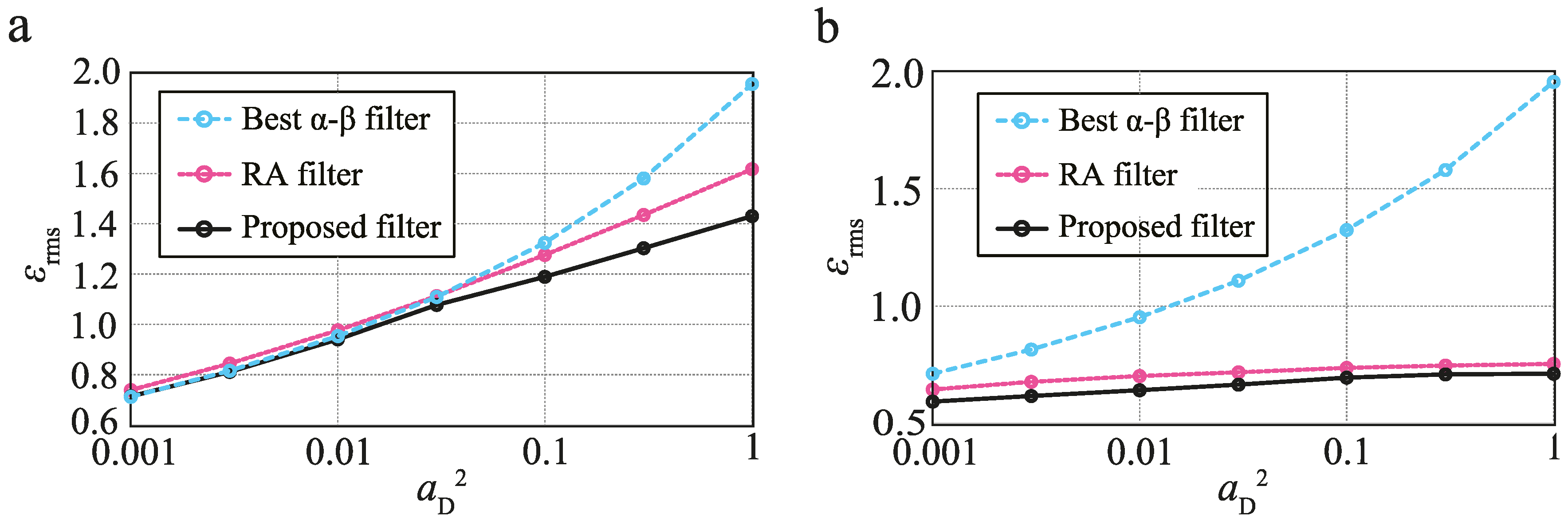
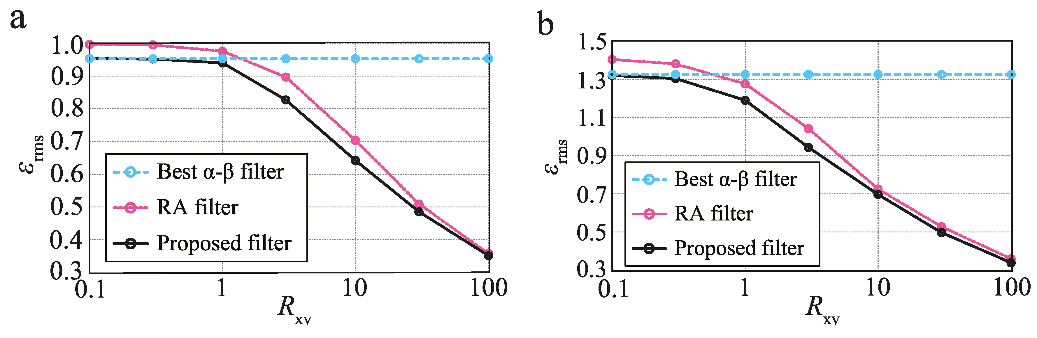
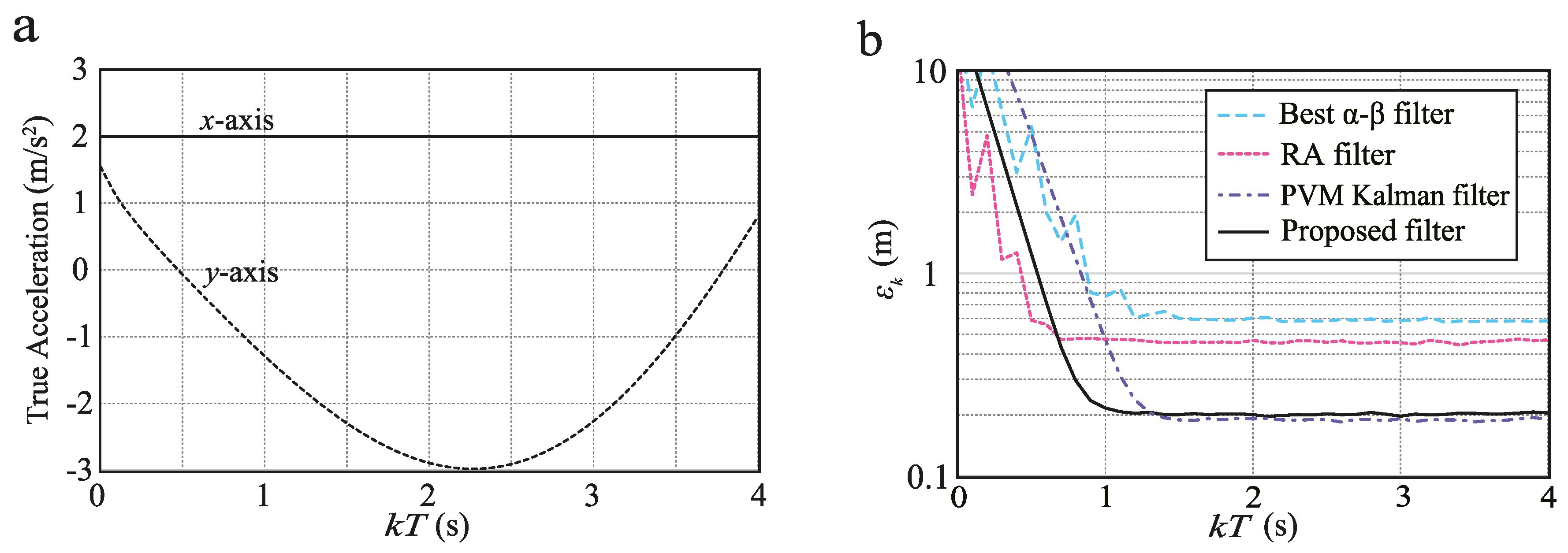
This section presents theoretical performance analyses of the $\alpha$-$\beta$-$\eta$-$\theta$ filter using the proposed design strategy. We compare the RMS index calculated using Equations (20), (26) and (28) for the following filters:

• Proposed filter: the $\alpha$-$\beta$-$\eta$-$\theta$ filter with the proposed strategy.
• RA filter: the $\alpha$-$\beta$-$\eta$-$\theta$ filter with the RA model using optimal q (from Equation (16)) with respect to the RMS index.
• Best $\alpha$-$\beta$ filter: the conventional $\alpha$-$\beta$ filter obtained with the proposed strategy, assuming $\eta =\theta =0$.

Comparison with the RA filter indicates the effectiveness of the proposed strategy (i.e., considering ${\mathit{Q}}_{\mathrm{gen}}$), and comparison with the best $\alpha$-$\beta$ filter illustrates the effectiveness of the velocity measurements. Note that the analysis in this section investigates the steady state performance, and this also corresponds to the steady state Kalman filter analysis. We assume that $B_{\mathrm{x}}$ and T are normalized to one.

6.1. Relationship between Performance and $a_{\mathrm{D}}$

Figure 1 shows the relationship between the design parameter $a_{\mathrm{D}}$ and the RMS index ${ϵ}_{\mathrm{rms}}$ for $R_{\mathrm{xv}}=1$ and 10. From Figure 1a, the proposed filter realizes the best performance for relatively large $a_{\mathrm{D}}$. This result verifies that the proposed strategy determines gains corresponding to a better covariance matrix of process noise than the RA filter. The proposed filter also achieves better performance compared with the best $\alpha$-$\beta$ filter, including small $a_{\mathrm{D}}$, and even for $R_{\mathrm{xv}}=1$, which means that the measurement accuracy of the position and velocity is the same. Furthermore, when the velocity measurement accuracy is high, the proposed filter achieves greater accuracy than the best $\alpha$-$\beta$ filter (Figure 1b). In addition, although the difference between the RA and proposed filters is small for $R_{\mathrm{xv}}=10$, the proposed filter also achieves the best performance.

6.2. Relationship between Performance and $R_{\mathrm{xv}}$

Figure 2 shows the relationship between $R_{\mathrm{xv}}$ and ${ϵ}_{\mathrm{rms}}$ for $a_{\mathrm{D}}^2=$ 0.01 and 0.1, and both cases exhibit the same trend. For both proposed and RA filters, better performance is achieved with better velocity measurement accuracy. The performance of the proposed filter is better than that of the best $\alpha$-$\beta$ filter including relatively small $R_{\mathrm{xv}}$ (the velocity measurement accuracy is low). In contrast, the performance of the RA filter is worse than that of the best $\alpha$-$\beta$ filter for small $R_{\mathrm{xv}}$, because the covariance matrix of the RA filter is limited to Equation (16). Moreover, by comparing Figure 2a,b, we see the superior effectiveness of the proposed filter for relatively large $a_{\mathrm{D}}$. These results indicate that the proposed filter is effective when the velocity measurement accuracy and/or target acceleration is relatively high.

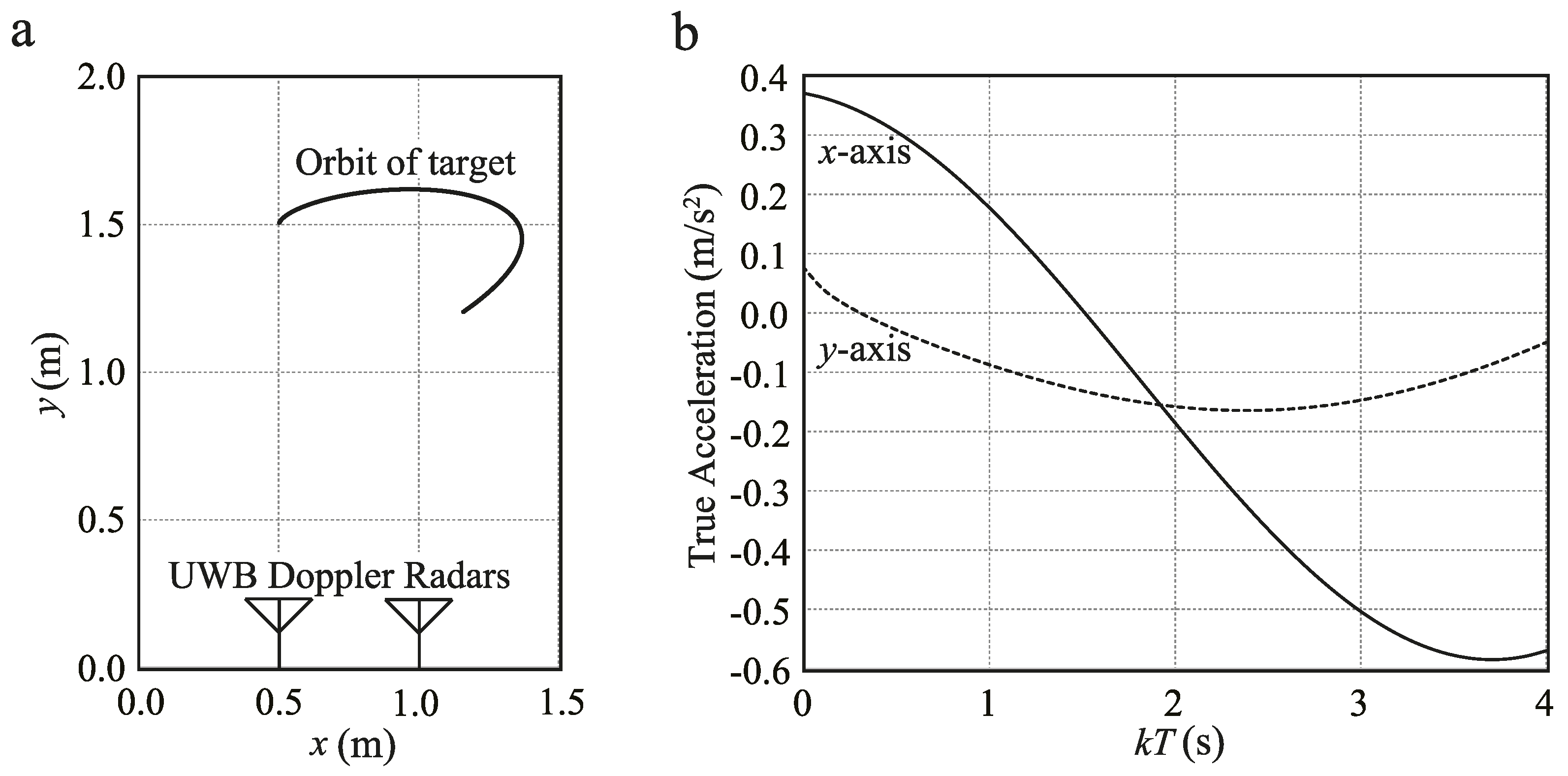
7. Application to UWB Doppler Radar Simulation

This section provides examples of the $\alpha$-$\beta$-$\eta$-$\theta$ filter designed with the proposed strategy for a realistic application to UWB Doppler radar tracking. Numerical simulations show the effectiveness of the proposed strategy. We consider two scenarios:

• Medium maneuvering target assuming simple near-field sensing.
• High maneuvering target assuming the target executes an abrupt motion.

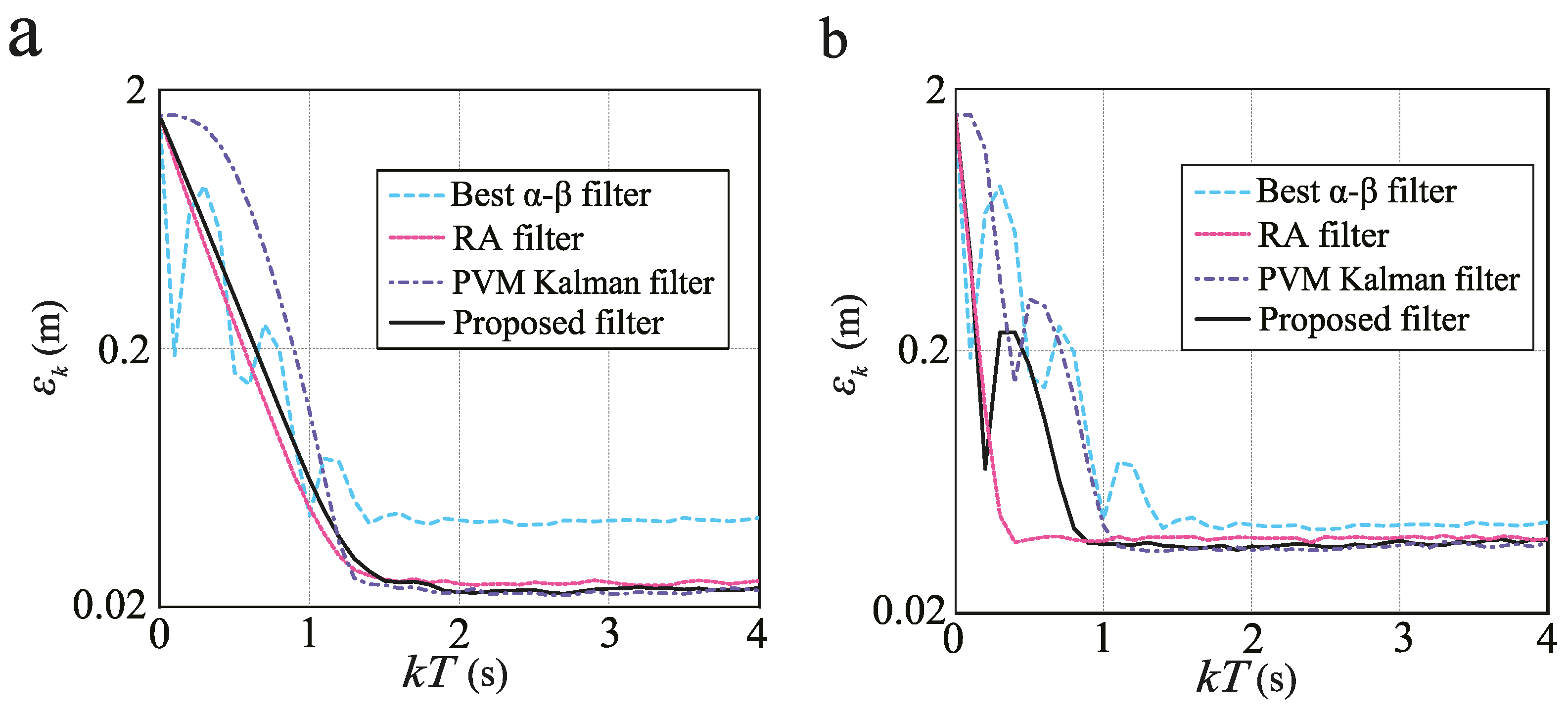
7.1. Tracking of Medium Maneuvering Target

7.1.1. Simulation Setup

First, we show the application examples for a maneuvering target that assumes near-field radar remote sensing for surveillance and robot monitoring systems. We simulate the UWB Doppler radar tracking [23,24,25] of a maneuvering target and compare the tracking errors of the filters assumed in the previous section and the PVM Kalman filter. For one-dimensional tracking assumed in the previous sections, the steady state performances of the PVM Kalman and the proposed filters are the same. However, for two-dimensional tracking assumed in this section, a difference in their tracking accuracy occurs because the Kalman filter considers correlations between the $x-y$ positions and velocities. Therefore, a comparison between the $\alpha$-$\beta$-$\eta$-$\theta$ filters and the PVM Kalman filter is also necessary.

Figure 3 shows the simulation scenario and the true acceleration of a target. The true target position is ($x_{\mathrm{t},k}$, $y_{\mathrm{t},k}$) = ($0.5+0.3kTsin(2\pi kT/10)$, $1.5+0.1{\left(kT\right)}^{1.2}cos(2\pi kT/12)$). Two-dimensional tracking in the x-y plane of the point target is assumed. We consider two Doppler radars located at $(x,y)=(0.5m,0)$ and $(1.0m,0)$. The sampling interval T is 100 ms, and the observation time is 4 s. The transmitted signal is a UWB pulse with a center frequency of 26.4 GHz and a bandwidth of 500 MHz. The received radar signals are calculated using ray tracing with the addition of Gaussian white noise. The radars measure position using ranging results [24] and measure velocity using the Doppler shift with the method presented in [25]. We determine a standard derivation for this noise to set $B_{\mathrm{x}}=0.{030}^2$ m${}^2$ and $B_{\mathrm{v}}=0.{10}^2$ m${}^2$/s${}^2$. These values are the averages along the two axes (x and y) and are set based on the experimental results in [23,24]. Thus, the $R_{\mathrm{xv}}$ of the assumed radar system is 9.0. For simplicity, we use this value for both axes. In addition, to evaluate the performance for smaller $R_{\mathrm{xv}}$, the case $R_{\mathrm{xv}}=1.0$ is generated by adding Gaussian white noise to the measured velocity data. $B_{\mathrm{v}}$ in this instance is 0.30${}^2$ m${}^2$/s${}^2$.

The $\alpha$-$\beta$ and $\alpha$-$\beta$-$\eta$-$\theta$ filters are implemented for each axis, for which we use the same gain. The implementation of the PVM Kalman filter is the same as in [27], and its covariance matrix for process noise is calculated from the optimal $\alpha$-$\beta$-$\eta$-$\theta$ filter gains designed with the proposed strategy using Equations (34)–(36). The initial values of the state vectors and the error covariance matrix of the PVM Kalman filter are all zero. Using the RMS prediction error calculated from 1000 Monte Carlo simulations, the performance is defined as:

$$\begin{array}{c}\hfill {ϵ}_k=\sqrt{\frac{1}{1000}\sum _{m=1}^{1000}\{{(x_{\mathrm{t},k}-x_{\mathrm{p},m,k})}^2+{(y_{\mathrm{t},k}-y_{\mathrm{p},m,k})}^2\}},\end{array}$$

(37)

where $x_{\mathrm{p},m,k}$ and $y_{\mathrm{p},m,k}$ are the predicted positions in the m-th Monte Carlo simulation.

7.1.2. Filter Design

The gain design for the UWB Doppler radar using the proposed strategy is presented here. We design an appropriate $a_{\mathrm{D}}$ and evaluate the resultant performance. We presume a rough approximate prediction of accelerations. For instance, when the maximum acceleration of the target in Figure 3b is approximately predicted as $a_{\mathrm{c}}=0.6$ m/s${}^2$, $a_{\mathrm{D}}^2$ is then 0.04 from Equation (31). Using this $a_{\mathrm{D}}^2$, the above radar settings of $R_{\mathrm{xv}}=9.0$ (T = 100 ms, $B_{\mathrm{x}}$ = 0.03${}^2$ m${}^2$ and $B_{\mathrm{v}}$ = 0.1${}^2$ m${}^2$/s${}^2$) and solving Equation (32), we have the optimal gains $\alpha$ = 0.315, $\beta$ = 0.00801, $\eta$ = 0.0721 and $\theta$ = 1.15. Optimal gains for other settings are similarly determined.

7.1.3. Evaluation Results

Figure 4 shows the simulation results for $a_{\mathrm{D}}^2=0.04$ ((a) $R_{\mathrm{xv}}$ = 9.0, (b) $R_{\mathrm{xv}}$ = 1.0). Clearly, the filters using velocity measurements achieve greater accuracy than the best $\alpha$-$\beta$ filter in both cases. For $R_{\mathrm{xv}}=9.0$, the mean steady state prediction RMS errors ($E[{ϵ}_k]$ in $2<kT<4$) of the RA, PVM Kalman and proposed filters are 2.48, 2.30 and 2.33 cm, respectively. These results indicate that the proposed filter achieves better accuracy than the RA filter even for realistic situations. Although the PVM Kalman filter is slightly better than the proposed filter, because it considers the correlated noise in the x- and y-axes, their errors are almost the same. This shows that the steady state performance of the PVM filter is close to that of the $\alpha$-$\beta$-$\eta$-$\theta$ filter, and the $\alpha$-$\beta$-$\eta$-$\theta$ filter analysis is effective in performance predictions of the PVM Kalman filters. The relationship of these filters is similar to the traditional $\alpha$-$\beta$ and position-only-measured Kalman filters. The computational load of the $\alpha$-$\beta$-$\eta$-$\theta$ filter is considerably smaller than that of the PVM Kalman filter; the mean calculation times for each k of the $\alpha$-$\beta$-$\eta$-$\theta$ and PVM Kalman filters are 14.0 and 38.1 $\mathsf{\mu }$s using an Intel Core i7-4600U [email protected] GHz 2.70 GHz processor and Scilab 5.5.0. This is because the $\alpha$-$\beta$-$\eta$-$\theta$ filter does not require the adaptive calculations of the gains and error covariance matrices. In addition, although the difference in steady state accuracy between the proposed and best $\alpha$-$\beta$ filters is small (Figure 4b), the proposed filter achieves better accuracy even for $R_{\mathrm{xv}}$=1. The mean steady state prediction RMS errors of the RA, PVM Kalman and proposed filters are 3.84, 3.61 and 3.68 cm, respectively, and these results lead to the same conclusions as those from Figure 4a. These results are matched to the analysis results presented in the previous section.

We next investigate the performance of the proposed filter for different values of $a_{\mathrm{c}}$ to assess appropriate settings.

Table 3. Steady state RMS prediction error of the proposed filter for various $a_{\mathrm{c}}$ ($R_{\mathrm{xv}}=9$).

${\mathit{a}}_{\mathbf{c}}$ (m/s${}^2$)	${\mathit{a}}_{\mathbf{d}}^2$	Mean Steady State RMS Error (cm)
0.1	0.00111	2.82
0.4	0.0178	2.32
0.6	0.040	2.33
1.0	0.111	2.57

shows the steady state RMS error ($E[{ϵ}_k]$ in $2<kT<4$) for different values of $a_{\mathrm{c}}$ for $R_{\mathrm{xv}}=9.0$; $a_{\mathrm{c}}=0.4$ m/s${}^2$ is assumed as a rough approximation for the mean acceleration of the target, and $a_{\mathrm{c}}=0.1$ and 1 m/s${}^2$ are considered as the order of the acceleration. The performance of the proposed filter deteriorates for $a_{\mathrm{c}}=0.1$ and 1 m/s${}^2$. This is because the difference between the true target accelerations and these very rough approximate accelerations is too large. This means that the proposed strategy requires some minimum degree of accuracy in target acceleration prediction to perform adequately. However, the $a_{\mathrm{c}}=0.4$ and 0.6 m/s${}^2$ cases have almost the same accuracy, implying that strict values of the target acceleration are in practice not required with UWB Doppler radars. As a method to obtain an approximated acceleration, communications of the tracking systems and the accelerometers embedded in targets can be considered. Many sensing targets have acceleration sensors, e.g., the robots and vehicles have inertial sensors, and humans have accelerometers embedded in smart phones. In the near future, the Internet-of-Things technology will make data communications between robots, smart phones and radar possible. Thus, we can obtain approximated acceleration based on this novel technology.

7.2. Tracking of High-Maneuvering Target

Finally, an application to high-maneuvering targets with relatively high accelerations is presented to clearly show the effectiveness of the proposed filter compared with the RA filter. Given the true target position of ($x_{\mathrm{t},k}$, $y_{\mathrm{t},k}$) = ($k^2{T}^2$, $20+{\left(kT\right)}^{1.5}cos(2\pi kT/10)$), the true acceleration is plotted in Figure 5a. Compared with the previous section, a high acceleration is assumed. We set $B_{\mathrm{x}}$ = 0.3${}^2$, $R_{\mathrm{xv}}$ = 1.0, $a_{\mathrm{c}}=3$ m/s${}^2$ and $a_{\mathrm{D}}$ = 1.0; other settings are the same as in the previous section.

Figure 5b shows the simulation results for the high-maneuvering target. The difference in the RMS prediction error between the RA and proposed filters becomes large compared with the moderate-maneuvering target assumed in the previous section. $E[{ϵ}_k]$ in $2<kT<4$ s of the best $\alpha$-$\beta$, RA, PVM Kalman and proposed filters are 0.589, 0.459, 0.190 and 0.201 m, respectively. Whereas the PVM Kalman filter is slightly better than the proposed filter for the same reason as for a moderate-maneuvering target, the proposed filter achieves greater accuracy than the RA filter. This is because the RA model cannot track the abrupt motion of the high-maneuvering target because of limitations in expressing process noise. In contrast, the proposed filter can set gains corresponding to the appropriate process noises to accurately track the high-maneuvering target. Our theoretical analyses presented in Figure 1a show that the performance difference between the assumed filters becomes large when $a_{\mathrm{D}}$ is relatively large. The above simulation results are consistent with these analyses. In addition, with respect to the steady state accuracy of the PVM Kalman and the proposed filter, the same result with the moderate-maneuvering target is obtained. Thus, the applicability to performance predictions of the PVM Kalman filters using the analysis of the $\alpha$-$\beta$-$\eta$-$\theta$ filter is clearly indicated with these simulation results.

8. Conclusions

We have proposed a gain design strategy for $\alpha$-$\beta$-$\eta$-$\theta$ filters and applied it to UWB Doppler radar simulations. Stability conditions and an efficient performance index (the RMS index) for the $\alpha$-$\beta$-$\eta$-$\theta$ filter were analytically derived, and a design strategy was presented based on minimization of the RMS index. We clarified the design parameters of the proposed strategy and examined their relationship with those of the PVM Kalman filter. Numerical analyses using the derived performance index showed that the designed $\alpha$-$\beta$-$\eta$-$\theta$ filter achieved better performance than the traditional $\alpha$-$\beta$ filter, as well as an $\alpha$-$\beta$-$\eta$-$\theta$ filter designed using the general RA model. Finally, a numerical simulation assuming a realistic UWB Doppler radar application verified the effectiveness of an $\alpha$-$\beta$-$\eta$-$\theta$ filter designed using the proposed strategy and the validity of the theoretical analyses. This simulation showed that the proposed strategy can be applied to realistic tracking systems by presetting several simple parameters, specifically an approximate acceleration and the radar measurement accuracy. Moreover, the possibility of the application to performance predictions for the PVM Kalman filter design was also indicated.

References

1. Wu, K.; Cai, Z.; Zhao, J.; Wang, Y. Target Tracking Based on a Nonsingular Fast Terminal Sliding Mode Guidance Law by Fixed-Wing UAV. Appl. Sci. 2017, 7, 333. [Google Scholar] [CrossRef]
2. Fan, Y.; Lu, F.; Zhu, W.; Bai, G.; Yan, L. A Hybrid Model Algorithm for Hypersonic Glide Vehicle Maneuver Tracking Based on the Aerodynamic Model. Appl. Sci. 2017, 7, 159. [Google Scholar] [CrossRef]
3. Li, W.; Sun, S.; Jia, Y.; Du, J. Robust unscented Kalman filter with adaptation of process and measurement noise covariances. Digit. Signal Process. 2016, 48, 93–103. [Google Scholar] [CrossRef]
4. Saho, K.; Masugi, M. Automatic Parameter Setting Method for an Accurate Kalman Filter Tracker Using an Analytical Steady-State Performance Index. IEEE Access 2015, 3, 1919–1930. [Google Scholar] [CrossRef]
5. Jin, B.; Jiu, B.; Su, T.; Liu, H.; Liu, G. Switched Kalman filter-interacting multiple model algorithm based on optimal autoregressive model for manoeuvring target tracking. IET Radar Sonar Navig. 2015, 9, 199–209. [Google Scholar] [CrossRef]
6. Martino, L.; Read, J.; Elvira, V.; Louzada, F. Cooperative Parallel Particle Filters for on-Line Model Selection and Applications to Urban Mobility. Digit. Signal Process. 2017, 60, 172–185. [Google Scholar] [CrossRef]
7. Drovandi, C.C.; McGree, J.; Pettitt, A.N. A sequential Monte Carlo algorithm to incorporate model uncertainty in Bayesian sequential design. J. Comput. Graph. Stat. 2014, 23, 324. [Google Scholar] [CrossRef] [Green Version]
8. Crouse, D.F. A general solution to optimal fixed-gain (α-β-γ etc.) filters. IEEE Signal Process. Lett. 2015, 22, 901–904. [Google Scholar] [CrossRef]
9. Bar-Shalom, Y.; Li, X.R. Estimation and Tracking: Principles, Techniques, and Software; Artech House Publishers: Boston, MA, USA, 1998. [Google Scholar]
10. Kalata, P.R. The Tracking Index: A Generalized Parameter for α-β and α-β-γ Target Trackers. IEEE Trans. Aerosp. Electron. Syst. 1984, AES-20, 174–182. [Google Scholar] [CrossRef]
11. Saho, K.; Masugi, M. Performance analysis of alpha-beta-gamma tracking filters using position and velocity measurements. EURASIP J. Adv. Signal Process. 2015, 2015, 35. [Google Scholar] [CrossRef]
12. Ekstrand, B. Some Aspects on Filter Design for Target Tracking. J. Control Sci. Eng. 2012, 2012. [Google Scholar] [CrossRef]
13. O’Shea, T.P.; Bamber, J.C.; Harris, E.J. Temporal regularization of ultrasound-based liver motion estimation for image-guided radiation therapy. Med. Phys. 2016, 43, 455–464. [Google Scholar] [CrossRef] [PubMed]
14. Khin, N.H.; Che, Y.F.; Eileen, S.M.L.; Liang, W.X. Alpha Beta Gamma Filter for Cascaded PID Motor Position Control. Procedia Eng. 2012, 41, 244–250. [Google Scholar]
15. Lee, Y.S.; Lee, H.J. Multiple object tracking for fall detection in real-time surveillance system. In Proceedings of the International Conference Advanced Communication Technology 2009 (ICACT2009), Phoenix Park, Korea, 15–18 February 2009; pp. 2308–2312. [Google Scholar]
16. Matsunami, I.; Nakamura, R.; Kajiwara, A. Target State Estimation Using RCS Characteristics for 26 GHz Short-Range Vehicular Radar. In Proceedings of the IEEE 2013 International Conference on Radar, Adelaide, SA, Australia, 9–12 September 2013; pp. 304–308. [Google Scholar]
17. Jatoth, R.K.; Gopisety, S.; Hussain, M. Performance Analysis of Alpha Beta Filter, Kalman Filter and Meanshift for Object Tracking in Video Sequences. Int. J. Image Graph. Signal Process. 2015, 7, 24–30. [Google Scholar] [CrossRef]
18. Abdelkrim, M.; Mohammed, D.; Mokhtar, K.; Abdelaziz, O. A simplified alpha-beta based Gaussian sum filter. AEU Int. J. Electron. Commun. 2013, 67, 313–318. [Google Scholar] [CrossRef]
19. Mohammed, D.; Mokhtar, K.; Abdelaziz, O.; Abdelkrim, M. A new IMM algorithm using fixed coefficients filters (fast IMM). AEU Int. J. Electron. Commun. 2009, 64, 1123–1127. [Google Scholar] [CrossRef]
20. Ma, K.; Chang, Y.; Li, H.; Gao, J. A new method of target tracking in Ultra-Short-Range Radar. In Proceedings of the International Conference on Computer Science and Network Technology (ICCSNT2013), Dalian, China, 12–13 October 2013; pp. 10–12. [Google Scholar]
21. Wang, Y. Feature point correspondence between consecutive frames based on genetic algorithm. Int. J. Robot. Autom. 2006, 21, 35–38. [Google Scholar] [CrossRef]
22. Yoo, J.C.; Kim, Y.S. Alpha-beta-tracking index (α-β-Λ) tracking filter. Signal Process. 2003, 83, 169–180. [Google Scholar] [CrossRef]
23. Dai, X.; Zhou, Z.; Zhang, J.J.; Davidson, B. Ultra-wideband radar-based accurate motion measuring: Human body landmark detection and tracking with biomechanical constraints. IET Radar Sonar Navig. 2015, 9, 154–163. [Google Scholar] [CrossRef]
24. Saho, K.; Sakamoto, T.; Sato, T.; Inoue, K.; Fukuda, T. Pedestrian imaging using UWB Doppler radar interferometry. IEICE Trans. Commun. 2013, E96-B, 613–623. [Google Scholar] [CrossRef]
25. Wang, Y.; Liu, Q.; Fathy, A.E. CW and pulse-Doppler radar processing based on FPGA for human sensing applications. IEEE Trans. Geosci. Remote Sens. 2013, 51, 3097–3107. [Google Scholar] [CrossRef]
26. Zhoua, G.; Wub, L.; Xiea, J.; Denga, W.; Quan, T. Constant turn model for statically fused converted measurement Kalman filters. Signal Process. 2015, 108, 400–411. [Google Scholar] [CrossRef]
27. Jahromi, M.J.; Bizaki, H.K. Target Tracking in MIMO Radar Systems Using Velocity Vector. J. Inf. Syst. Telecommun. 2014, 2, 150–158. [Google Scholar]
28. Geetha, B.; Ramachandra, K.V. A Three State Kalman Filter with Range and Range-Rate Measurements. Int. J. Comput. Appl. 2013, 3, 85–101. [Google Scholar]
29. Yoon, J.H.; Kim, D.Y.; Bae, S.H.; Shin, V. Joint Initialization and Tracking of Multiple Moving Objects Using Doppler Information. IEEE Trans. Signal Process. 2011, 59, 3447–3452. [Google Scholar] [CrossRef]
30. Saho, K. Fundamental properties and optimal gains of a steady state velocity measured α-β tracking filter. Adv. Remote Sens. 2014, 3, 61–76. [Google Scholar] [CrossRef]
31. Sudano, J.J. The alpha-beta-eta-theta tracker with a random acceleration process noise. In Proceedings of the IEEE National Aerospace and Electronics Conference (NEACON2000), Dayton, OH, USA, 10–12 October 2000; pp. 165–171. [Google Scholar]
32. Jury, E.I. Theory and Application of the z-Transform Method; John Wiley and Sons: NewYork, NY, USA, 1964. [Google Scholar]
33. Baldi, P. Gradient Descent Learning Algorithm Overview: A General Dynamical Systems Perspective. IEEE Trans. Neural Netw. 1995, 6, 182–195. [Google Scholar] [CrossRef] [PubMed]
34. Gelb, A. Applied Optimal Estimation; The M.I.T. PRESS: Cambridge, MA, USA, 1974. [Google Scholar]
Figure 1. Relationship between a D and ϵ rms for (a) R xv = 1 and (b) R xv = 10 ; RA: random-acceleration.
Applsci 07 00758 g001
Figure 2. Relationship between R xv and ϵ rms for (a) a D 2 = 0 . 01 and (b) a D 2 = 0 . 1 .
Applsci 07 00758 g002
Figure 3. UWB Doppler radar simulation scenario: (a) radar positions and true orbit; (b) true acceleration; UWB: ultra-wideband.
Applsci 07 00758 g003
Figure 4. Simulation results for (a) R xv = 9 and (b) R xv = 1 ; PVM: position-velocity-measured.
Applsci 07 00758 g004
Figure 5. Simulation assuming a high-maneuvering target: (a) true acceleration; (b) results.
Applsci 07 00758 g005