Computational Vibroacoustics in Low- and Medium- Frequency Bands: Damping, ROM, and UQ Modeling

Abstract

Within the framework of the state-of-the-art, this paper presents a summary of some common research works carried out by the authors concerning computational methods for the prediction of the responses in the frequency domain of general linear dissipative vibroacoustics (structural-acoustic) systems for liquid and gas in the low-frequency (LF) and medium-frequency (MF) domains, including uncertainty quantification (UQ) that plays an important role in the MF domain. The system under consideration consists of a deformable dissipative structure, coupled with an internal dissipative acoustic fluid including a wall acoustic impedance, and surrounded by an infinite acoustic fluid. The system is submitted to given internal and external acoustic sources and to prescribed mechanical forces. An efficient reduced-order computational model (ROM) is constructed using a finite element discretization (FEM) for the structure and the internal acoustic fluid. The external acoustic fluid is treated using a symmetric boundary element method (BEM) in the frequency domain. All the required modeling aspects required for the analysis in the MF domain have been introduced, in particular the frequency-dependent damping phenomena and model uncertainties. An industrial application to a complex computational vibroacoustic model of an automobile is presented.

1. Introduction

This paper presents a summary of some common research works carried out by the authors concerning computational methods for the prediction of the responses in the frequency domain of general linear dissipative vibroacoustics (structural-acoustic) systems for liquid and gas in the low- frequency (LF) and medium-frequency (MF) domains, including uncertainty quantification (UQ) that plays an important role in the MF domain. The contribution of this paper is the presentation of an efficient computational methodology adapted to large-scale computational vibroacoustic models which corresponds to a combination of established methods, and an application of this computational methodology is presented for an industrial vibroacoustic system. Considering all the aspects that are developed in this paper in order to present a complete strategy for the modeling and computational approaches—external acoustic fluid modeling, internal acoustic fluid including a dissipation term and frequency-dependent wall impedance, structure with frequency-dependent constitutive equation, reduced-order model for weak and strong coupling between the structure and the internal acoustic fluid, complete methodology for uncertainty quantification—a synthetic presentation has been adopted for readability, and we refer the reader to the given appropriate bibliography for the details. Nevertheless, since the model uncertainties induced by the modeling errors—which cannot be taken into account by using the usual probabilistic parametric approach of uncertain parameters or of other deterministic approaches of uncertainties—is relatively novel for the readers who are not familiarized with such a formulation, this part is more detailed in terms of equations.

More specifically, this paper is devoted to computational methods for the prediction of the frequency responses of linear dissipative vibroacoustic (structural-acoustic) systems in the low- and medium-frequency ranges. The vibroacoustic system consists of a deformable dissipative structure, coupled with a bounded internal dissipative acoustic fluid including a wall acoustic impedance, immersed in an unbounded acoustic fluid, and submitted to internal and external acoustic sources, as well as mechanical forces.

Computational vibroacoustic predictions play an important and increasing role in analyzing industrial complex systems, and many works have been published in this field.

The physics on which the computational vibroacoustics formulations are based can be found in numerous books, such as in [1,2,3,4,5,6,7,8,9,10,11].

For the spatial discretization of structures and bounded internal acoustic fluids, the computational vibroacoustics are generally based on the finite element method (FEM) (see for instance [12,13,14,15], and [16] for the corresponding isogeometric formulation).

For the spatial discretization of the unbounded external acoustic fluid, either finite element method or boundary element method (BEM) are used. Concerning the use of the local discretization of the unbounded external acoustic fluid, we refer the reader to [17,18,19,20,21,22,23,24,25,26], and for the BEM that is based on the finite element discretization of the boundary integral equation methods, let us cite [27,28,29,30,31,32,33,34,35,36,37]. Concerning the BEMs that are specifically devoted to the unbounded external acoustic fluid, we refer the reader to [38,39,40,41,42,43,44,45,46,47,48].

Reduced-order models (ROMs) are very attractive and efficient for analyzing large computational vibroacoustics models that have a significant number of design parameters—also called parametric high-dimensional computational models (HDMs)—for design and optimization, for constructing online models for active control, and for taking uncertainties into account. Particularly for parametric nonlinear HDMs, many approaches which can also be applied to parametric linear HDMs have been proposed, including hyper-reduced ROM, which guarantees feasibility [49,50,51,52,53,54,55,56,57,58,59,60,61]. With these methods, the parameter admissible space must be sampled at a few points using a greedy sampling algorithm (e.g., [62]), and a set of problems must be solved, yielding a set of parametric solution snapshots. This generally results from a proper orthogonal decomposition (POD), which are compressed using, for example, singular value decomposition (SVD) to construct a global reduced-order basis (ROB). For linear vibroacoustic HDMs, the most common choice for the parametric ROB consists of taking the modes of the different parts that constitute the vibroacoustic system (e.g., the elastic modes of the structure and the acoustic modes of the internal acoustic fluid)[41,63,64,65,66,67,68,69,70,71,72,73,74].

The design of a vibroacoustic system is used to manufacture a real system and to construct a nominal computational model with the methodologies listed above, and which will be presented in the next sections. In practice, the real system can exhibit variabilities in its responses due to fluctuations in the manufacturing process and due to small variations of the configuration around a nominal configuration associated with the design. The vibroacoustic computational model has parameters such as geometry, mechanical properties, and boundary conditions, which can be uncertain, inducing uncertainties in the computational model parameters. On the other hand, the modeling process induces some modeling errors defined as the model uncertainties. It is important to consider both the model-parameters uncertainties and the modeling uncertainties in order to improve the predictions. Two main types of approaches can be used to model uncertainties in the framework of the probability theory [75]. The first is the parametric probabilistic approach, which consists of modeling the uncertain parameters by random variables (e.g., [75,76,77,78,79,80,81,82,83,84]), but which does not have the capability to take modeling uncertainties into account. Two main methods can then be used to take them into account. The first is the output-prediction-error method, which requires experimental data [85,86] and uses the Bayesian method [87,88], but for which the computational model cannot be updated using experimental data, which constitutes a lock for robust design and optimization. The second one is the nonparametric probabilistic approach of modeling uncertainties induced by modeling errors proposed in [75,89,90,91], based on the maximum entropy principle [92] in the context of Information Theory [93] and on the random matrix theory [94], and extended for nonlinear dynamical systems in [95].

The outline of this paper is the following:

• Statement of the problem in the frequency domain.
• External inviscid acoustic fluid equations in the frequency domain and acoustic impedance boundary operator.
• Internal dissipative acoustic fluid equations in the frequency domain.
• Structure equations with frequency-dependent constitutive equation.
• Boundary value problem in terms of the structural displacement and the internal pressure field.
• Vibroacoustic computational model.
• Reduced-order vibroacoustic computational model.
• Uncertainty quantification for the vibroacoustic computational model.
• Experimental validation with a complex computational vibroacoustic model of an automobile.

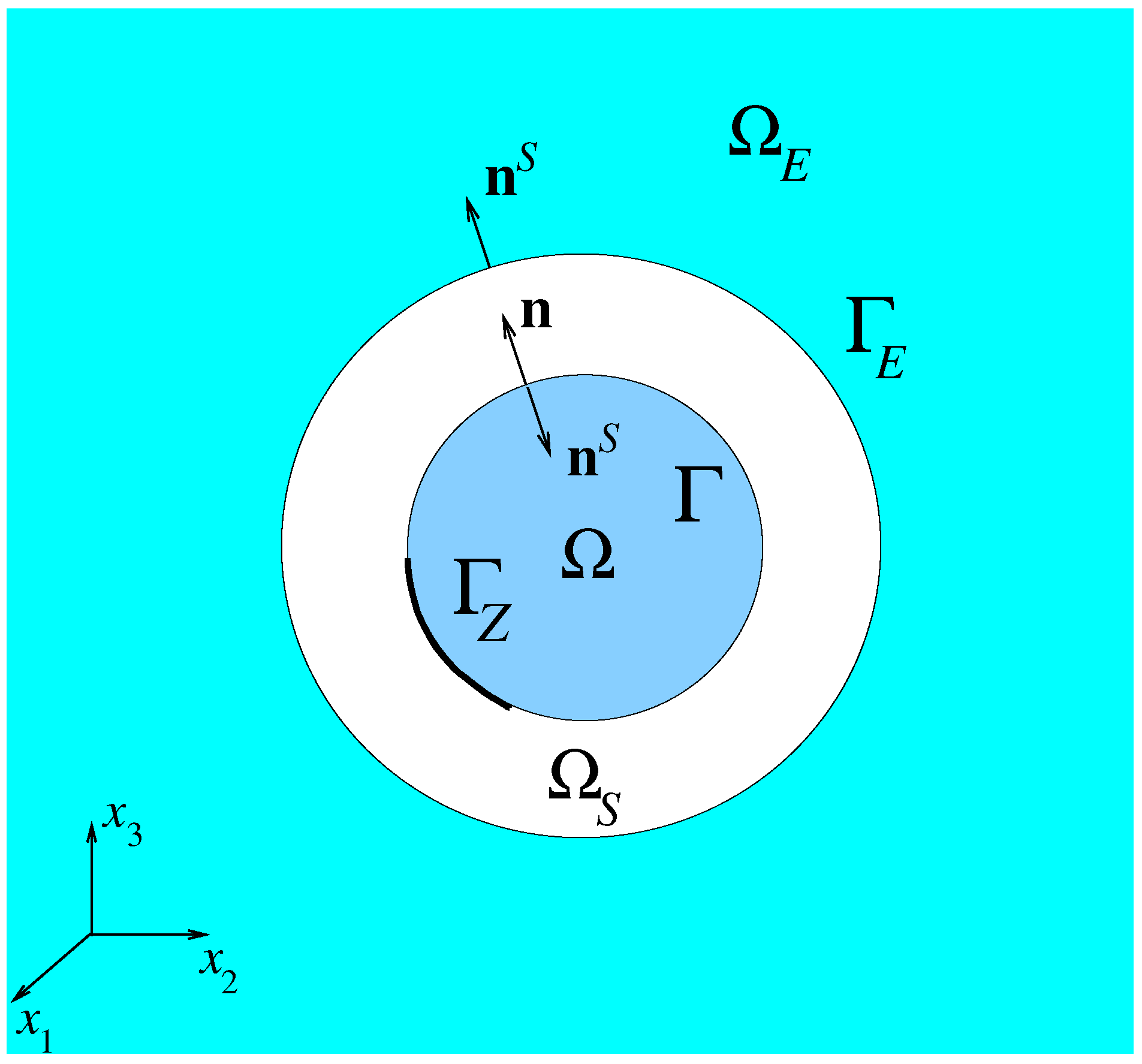
2. Statement of the Problem in the Frequency Domain

The physical space ${\mathbb{R}}^3$ refers to a cartesian reference system, and the generic point of ${\mathbb{R}}^3$ is denoted by $\mathbf{x}=(x_1,x_2,x_3)$. For any function $f(\mathbf{x})$, the notation $f{,}_j$ designates the partial derivative with respect to $x_j$. The classical convention for summations over repeated Latin indices is used, but not over Greek indices. The vibration problem is formulated in the frequency domain. Therefore, the Fourier transform is introduced for various quantities involved. For instance, for the displacement field $(\mathbf{x},t)\mapsto \mathbf{u}(\mathbf{x},t)$, the simplified notation $(\mathbf{x},\omega )\mapsto \mathbf{u}(\mathbf{x},\omega )={\int }_{-\infty }^{+\infty }{e}^{-i\omega t}\mathbf{u}(\mathbf{x},t)dt$ is introduced and consists of using the same symbol for a quantity and its Fourier transform, in which the circular frequency $\omega$ (rad/s) is real. The vibroacoustic system is assumed to be in linear vibrations around a static equilibrium state taken as a natural state at rest.

Structure. In general, the structure of a complex vibroacoustic system is composed of a main part called the master structure that is accessible to conventional modeling including uncertainties modeling, and a secondary part called the fuzzy substructure related to the structural complexity and including for example many equipment units attached to the master structure. In the present paper, we will not consider fuzzy substructures, and concerning fuzzy structure theory, we refer the reader to Chapter 15 of [41] for a synthesis, and to [96] for an extension of the theory to the modeling of an uncertain complex vibroacoustic system with fuzzy interface. At equilibrium, the structure occupies the three-dimensional bounded domain ${\mathsf{\Omega }}_S$ with a boundary $\partial {\mathsf{\Omega }}_S$ that is made up of a part ${\mathsf{\Gamma }}_E$ that is the coupling interface between the structure and the external acoustic fluid, a part $\mathsf{\Gamma }$ that is a coupling interface between the structure and the internal acoustic fluid, and finally, a part ${\mathsf{\Gamma }}_Z$ that is another part of the coupling interface between the structure and the internal acoustic fluid with acoustic properties. The structure is assumed to be free (free-free structure). The outward unit normal to $\partial {\mathsf{\Omega }}_S$ is denoted as ${\mathbf{n}}^S=(n_1^S,n_2^S,n_3^S)$ (see Figure 1). In ${\mathsf{\Omega }}_S$, the displacement field is denoted by $\mathbf{u}(\mathbf{x},\omega )=(u_1(\mathbf{x},\omega ),u_2(\mathbf{x},\omega ),u_3(\mathbf{x},\omega ))$. A surface force field $\mathbf{G}(\mathbf{x},\omega )=(G_1(\mathbf{x},\omega ),G_2(\mathbf{x},\omega ),$$G_3(\mathbf{x},\omega ))$ is given on $\partial {\mathsf{\Omega }}_S$, and a body force field $\mathbf{g}(\mathbf{x},\omega )=(g_1(\mathbf{x},\omega ),$$g_2(\mathbf{x},\omega ),g_3(\mathbf{x},\omega ))$ is given in ${\mathsf{\Omega }}_S$. The structure is a dissipative medium for which the frequency-dependent constitutive equation is detailed in Appendix A.

Figure 1. Geometry of the vibroacoustic system.

Internal dissipative acoustic fluid. Let $\mathsf{\Omega }$ be the internal bounded domain filled with a dissipative acoustic fluid (gas or liquid) that is described in Section 4. The boundary $\partial \mathsf{\Omega }$ of $\mathsf{\Omega }$ is $\mathsf{\Gamma }\cup {\mathsf{\Gamma }}_Z$. The outward unit normal to $\partial \mathsf{\Omega }$ is denoted by $\mathbf{n}=(n_1,n_2,n_3)$, and we have $\mathbf{n}=-{\mathbf{n}}^S$ on $\partial \mathsf{\Omega }$ (see Figure 1). The acoustic properties of boundary ${\mathsf{\Gamma }}_Z$ are modeled by a wall acoustic impedance $Z(\mathbf{x},\omega )$ satisfying the hypotheses defined in Section 4.2. In $\mathsf{\Omega }$, the pressure field is denoted by $p(\mathbf{x},\omega )$ and the velocity field by $\mathbf{v}(\mathbf{x},\omega )$. It is assumed that there is no Dirichlet boundary condition on any part of $\partial \mathsf{\Omega }$. An acoustic source density $Q(\mathbf{x},\omega )$ is given inside $\mathsf{\Omega }$.

External inviscid acoustic fluid. The structure is surrounded by an external inviscid acoustic fluid (gas or liquid) that is detailed in Appendix B. The fluid occupies the infinite three-dimensional domain ${\mathsf{\Omega }}_E$ whose boundary $\partial {\mathsf{\Omega }}_E$ is ${\mathsf{\Gamma }}_E$. The inward unit normal to $\partial {\mathsf{\Gamma }}_E$ is ${\mathbf{n}}^S$, defined above (see Figure 1). In ${\mathsf{\Omega }}_E$, the pressure field is denoted by $p_E(\mathbf{x},\omega )$. There is no Dirichlet boundary condition on ${\mathsf{\Gamma }}_E$. An acoustic source density $Q_E(\mathbf{x},\omega )$ is given in ${\mathsf{\Omega }}_E$. This acoustic source density induces a pressure field $p_{\mathrm{given}}(\omega )$ on ${\mathsf{\Gamma }}_E$ (defined in Appendix B). For the sake of brevity, the case of an incident plane wave is not considered here, and the reader is referred to [41] for this case.

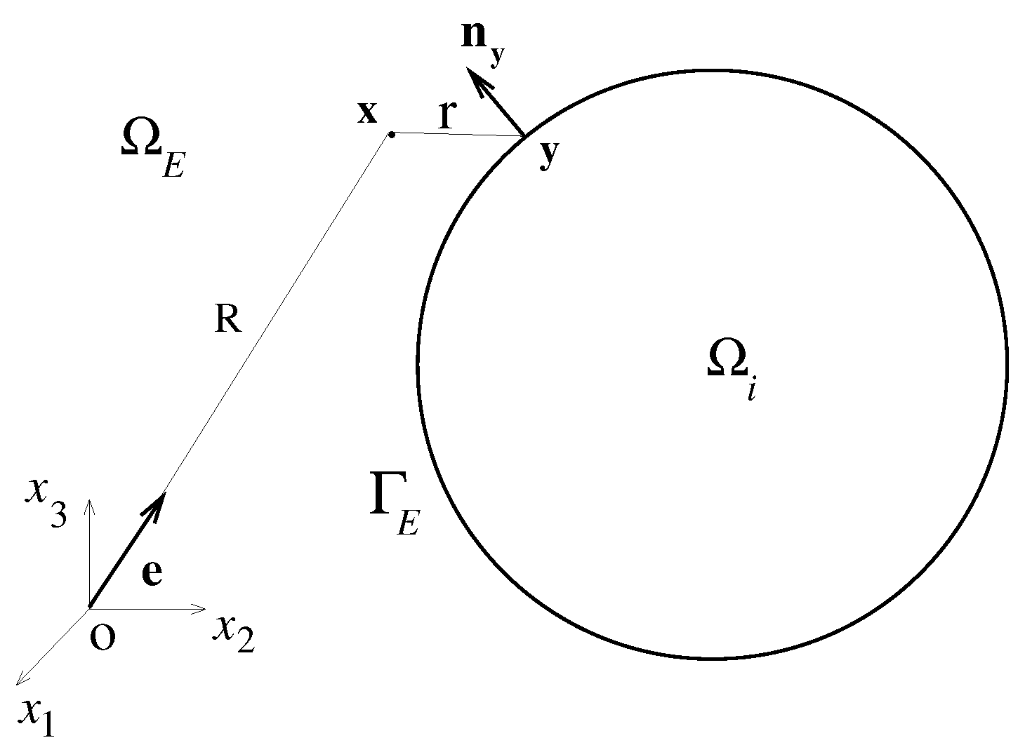
3. External Inviscid Acoustic Fluid Equations in the Frequency Domain and Acoustic Impedance Boundary Operator

Let ${\rho }_{\mathrm{E}}$ and $c_{\mathrm{E}}$ be the constant mass density and the constant speed of sound of the external acoustic fluid at equilibrium. Let $k=\omega /c_{\mathrm{E}}$ be the wave number at frequency $\omega$. The pressure is the solution of the classical exterior Neumann problem related to the Helmholtz equation with a source term [2,3,4,41],

$${\mathbf{\nabla }}^2{p}_E+k^2{p}_E=-i\omega Q_E\mathrm{in}{\mathsf{\Omega }}_E,$$

(1)

$$\frac{\partial p_E}{\partial {\mathbf{n}}^S}={\omega }^2{\rho }_E\mathbf{u}·{\mathbf{n}}^S\mathrm{on}{\mathsf{\Gamma }}_E,$$

(2)

$$|p_E|=O(\frac{1}{R}),\left|\frac{\partial p_E}{\partial R}+ik{p}_E\right|=O(\frac{1}{R^2}),$$

(3)

with $R=\parallel \mathbf{x}\parallel \to +\infty$, where $\partial /\partial R$ is the derivative in the radial direction and where $\mathbf{u}·{\mathbf{n}}^S$ is the normal displacement field on ${\mathsf{\Gamma }}_E$ induced by the deformation of the structure. Equation (3) corresponds to the outward Sommerfeld radiation condition at infinity. In Appendix B, it is shown that the value $p_E{|}_{{\mathsf{\Gamma }}_E}$ of the pressure field $p_E$ on the external fluid–structure interface ${\mathsf{\Gamma }}_E$ is related to the given external pressure field $p_{\mathrm{given}}{|}_{{\mathsf{\Gamma }}_E}$ on ${\mathsf{\Gamma }}_E$ and to the normal displacement field $\mathbf{u}(\omega )·{\mathbf{n}}^S$ on the external fluid–structure interface ${\mathsf{\Gamma }}_E$ by the equation

$$p_E{{|}_{{}_{{\mathsf{\Gamma }}_E}}(\omega )=p_{\mathrm{given}}|}_{{}_{{\mathsf{\Gamma }}_E}}(\omega )+i\omega {\mathbf{Z}}_{{\mathsf{\Gamma }}_E}(\omega )\{\mathbf{u}(\omega )·{\mathbf{n}}^S\},$$

(4)

in which ${\mathbf{Z}}_{{\mathsf{\Gamma }}_E}(\omega )$ is the acoustic impedance boundary operator. It can be proven that for all given real $\omega$ and for all given $\mathbf{u}·{\mathbf{n}}^S$ sufficiently regular on ${\mathsf{\Gamma }}_E$, the boundary value problem defined by Equations (1)–(3) (e.g., [97,98]) admits a unique solution.

4. Internal Dissipative Acoustic Fluid Equations in the Frequency Domain

4.1. Internal Dissipative Acoustic Fluid Equations

The internal fluid is called a dissipative acoustic fluid, and is assumed to be homogeneous, compressible, dissipative, and at rest in the reference configuration. This dissipative acoustic fluid—for which the dissipation due to thermal conduction is neglected and for which the motions are assumed to be irrotational—is driven by the Helmholtz equation with an additional internal dissipative term. For additional details concerning dissipation in acoustic fluids, we refer the reader to [2,4,6,9]. Let ${\rho }_0$ be the mass density and let $c_0$ be the constant speed of sound in the acoustic fluid at equilibrium in the reference configuration $\mathsf{\Omega }$. The Helmholtz equation with a dissipative term and a source term Q is written as [41]

$$\frac{1}{{\rho }_0}{\mathbf{\nabla }}^{2}p+i\omega \frac{\tau }{{\rho }_0}{\mathbf{\nabla }}^{2}p+\frac{{\omega }^2}{{\rho }_0{c}_0^2}p=-\frac{1}{{\rho }_0}(i\omega Q-\tau c_0^2{\mathbf{\nabla }}^{2}Q)\mathrm{in}\mathsf{\Omega },$$

(5)

in which $\tau$ is given by

$$\tau =\frac{1}{{\rho }_0{c}_0^2}\left(\frac{4}{3}\eta +\zeta \right)>0.$$

(6)

The constant $\eta$ is the dynamic viscosity, $\nu =\eta /{\rho }_0$ is the kinematic viscosity, and $\zeta$ is the second viscosity which can depend on $\omega$. Therefore, $\tau$ can depend on frequency $\omega$. To simplify the notation, we write $\tau$ instead of $\tau (\omega )$. Taking $\tau =0$ in Equation (5) yields the usual Helmholtz equation with an acoustic source for wave propagation in an inviscid acoustic fluid. It should be noted that the dissipation term is proportional to ${\mathbf{\nabla }}^{2}p$ and not to p (what modifies the boundary condition defined after), and that the acoustic source term exhibits a ${\mathbf{\nabla }}^{2}Q$ term.

4.2. Boundary Conditions

(i) Let $\mathbf{v}(\mathbf{x},\omega )$ be the velocity in the acoustic fluid. The interface condition on $\mathsf{\Gamma }$ for the inviscid dissipative acoustic fluid is written as $\mathbf{v}·\mathbf{n}=i\omega \mathbf{u}·\mathbf{n}$ on $\mathsf{\Gamma }$. In terms of p, the Neumann boundary condition is written as

$$(1+i\omega \tau )\frac{\partial p}{\partial \mathbf{n}}={\omega }^2{\rho }_0\mathbf{u}·\mathbf{n}+\tau c_0^2\frac{\partial Q}{\partial \mathbf{n}}\mathrm{on}\mathsf{\Gamma }.$$

(7)

(ii) The wall acoustic impedance on ${\mathsf{\Gamma }}_Z$ is defined by the following constitutive equation:

$$p(\mathbf{x},\omega )=Z(\mathbf{x},\omega )\{\mathbf{v}(\mathbf{x},\omega )·\mathbf{n}-i\omega \mathbf{u}(\mathbf{x},\omega )·\mathbf{n}\},$$

(8)

in which $Z(\mathbf{x},\omega )$ is the wall acoustic impedance defined for $\mathbf{x}\in {\mathsf{\Gamma }}_Z$, with complex values. Wall acoustic impedance $Z(\mathbf{x},\omega )$ must satisfy appropriate conditions in order to ensure that the problem is correctly stated (see [41] for a general formulation). In terms of p, the Neumann boundary condition on ${\mathsf{\Gamma }}_Z$ is written as

$$(1+i\omega \tau )\frac{\partial p}{\partial \mathbf{n}}={\omega }^2{\rho }_0\mathbf{u}·\mathbf{n}-i\omega {\rho }_0\frac{p}{Z}+\tau c_0^2\frac{\partial Q}{\partial \mathbf{n}}\mathrm{on}{\mathsf{\Gamma }}_Z.$$

(9)

4.3. Case of a Free Surface for a Liquid

In a case of an acoustic liquid with a free surface ${\mathsf{\Gamma }}_0$, neglecting gravity effects, the following Dirichlet condition is written as

$$p=0\mathrm{on}{\mathsf{\Gamma }}_0.$$

(10)

5. Structure Equations with Frequency-Dependent Constitutive Equation

Structure Equations in the Frequency Domain

The equation of the structure occupying domain ${\mathsf{\Omega }}_S$ is written as

$$-{\omega }^2{\rho }_{\mathrm{S}}{u}_i-{\sigma }_{ij,j}(\mathbf{u})=g_i\mathrm{in}{\mathsf{\Omega }}_S,$$

(11)

in which ${\rho }_{\mathrm{S}}(\mathbf{x})$ is the mass density of the structure. For a linear viscoelastic model, the symmetric stress tensor is written as

$${\sigma }_{ij}(\mathbf{u})=(a_{ijkh}(\omega )+i\omega b_{ijkh}(\omega )){\epsilon }_{kh}(\mathbf{u}),$$

(12)

in which the symmetric strain tensor ${\epsilon }_{kh}(\mathbf{u})$ is such that

$${\epsilon }_{kh}(\mathbf{u})=\frac{1}{2}(u_{k,h}(\mathbf{x},\omega )+u_{h,k}(\mathbf{x},\omega )),$$

(13)

and where the tensors $a_{ijkh}(\omega )$ and $b_{ijkh}(\omega )$ depend on $\omega$ and are detailed in Appendix A for the LF and MF ranges.

On the fluid–structure external interface ${\mathsf{\Gamma }}_E$, the boundary condition is such that

$${\sigma }_{ij}(\mathbf{u})n_j^S=G_i-p_E{|}_{{}_{{\mathsf{\Gamma }}_E}}{n}_i^S\mathrm{on}{\mathsf{\Gamma }}_E.$$

(14)

Using Equation (4) yields

$${\sigma }_{ij}(\mathbf{u})n_j^S=G_i-p_{\mathrm{given}}{|}_{{}_{{\mathsf{\Gamma }}_E}}{n}_i^S-i\omega {\mathbf{Z}}_{{\mathsf{\Gamma }}_E}(\omega )\{\mathbf{u}·{\mathbf{n}}^S\}{n}_i^S\mathrm{on}{\mathsf{\Gamma }}_E.$$

(15)

Since ${\mathbf{n}}^S=-\mathbf{n}$, the boundary condition on $\mathsf{\Gamma }\cup {\mathsf{\Gamma }}_Z$ is written as

$${\sigma }_{ij}(\mathbf{u})n_j^S=G_i+p{n}_i\mathrm{on}\mathsf{\Gamma }\cup {\mathsf{\Gamma }}_Z,$$

(16)

in which p is the internal acoustic pressure field defined in Section 4.

6. Boundary Value Problem in Terms of $\{\mathbf{u},\mathit{p}\}$

The boundary value problem in terms of $\{\mathbf{u},p\}$ is written as follows. For all real $\omega$ and for given $\mathbf{G}(\omega )$, $\mathbf{g}(\omega )$, $p_{\mathrm{given}}{|}_{{\mathsf{\Gamma }}_E}(\omega )$, and $Q(\omega )$, find $\mathbf{u}(\omega )$ and $p(\omega )$, such that

$$-{\omega }^2{\rho }_{\mathrm{S}}\mathbf{u}-\mathrm{div}\sigma (\mathbf{u})=\mathbf{g}\mathrm{in}{\mathsf{\Omega }}_S,$$

(17)

$$\sigma (\mathbf{u}){\mathbf{n}}^S=\mathbf{G}-p_{\mathrm{given}}{|}_{{}_{{\mathsf{\Gamma }}_E}}{\mathbf{n}}^S-i\omega {\mathbf{Z}}_{{\mathsf{\Gamma }}_E}(\omega )\{\mathbf{u}·{\mathbf{n}}^S\}{\mathbf{n}}^S\mathrm{on}{\mathsf{\Gamma }}_E,$$

(18)

$$\sigma (\mathbf{u}){\mathbf{n}}^S=\mathbf{G}+p\mathbf{n}\mathrm{on}\mathsf{\Gamma }\cup {\mathsf{\Gamma }}_Z.$$

(19)

$$-\frac{{\omega }^2}{{\rho }_0{c}_0^2}p-i\omega \frac{\tau }{{\rho }_0}{\mathbf{\nabla }}^{2}p-\frac{1}{{\rho }_0}{\mathbf{\nabla }}^{2}p=\frac{1}{{\rho }_0}(i\omega Q-\tau c_0^2{\mathbf{\nabla }}^{2}Q)\mathrm{in}\mathsf{\Omega }.$$

(20)

$$(1+i\omega \tau )\frac{\partial p}{\partial \mathbf{n}}={\omega }^2{\rho }_0\mathbf{u}·\mathbf{n}+\tau c_0^2\frac{\partial Q}{\partial \mathbf{n}}\mathrm{on}\mathsf{\Gamma }.$$

(21)

$$(1+i\omega \tau )\frac{\partial p}{\partial \mathbf{n}}={\omega }^2{\rho }_0\mathbf{u}·\mathbf{n}-i\omega {\rho }_0\frac{p}{Z}+\tau c_0^2\frac{\partial Q}{\partial \mathbf{n}}\mathrm{on}{\mathsf{\Gamma }}_Z.$$

(22)

In the case of a free surface ${\mathsf{\Gamma }}_0$ in the internal acoustic cavity (see Section 4.3), the boundary condition defined by Equation (10) must be added.

Remarks

• Equation (17) corresponds to the structure equation (see Equations (11)–(13)), in which ${\{\mathrm{div}\sigma (\mathbf{u})\}}_i={\sigma }_{ij,j}(\mathbf{u})$.
• Equations (18) and (19) are the boundary conditions for the structure (see Equations (15) and (16)).
• Equation (20) corresponds to the internal dissipative acoustic fluid equation (see Equation (5)).
• Equations (21) and (22) are the boundary conditions for the acoustic cavity (see Equations (7) and (9)).
• It is important to note that the external acoustic pressure field $p_E$ has been eliminated as a function of $\mathbf{u}$ using the acoustic impedance boundary operator ${\mathbf{Z}}_{{\mathsf{\Gamma }}_E}(\omega )$ (see Equation (4) of Section 3 and Appendix B), while the internal acoustic pressure field p is kept.

7. Vibroacoustic Computational Model

The finite element method is used to construct the spatial discretization of the variational formulation of the boundary value problem defined by Equations (17)–(22), with the additional boundary condition defined by Equation (10) in the case of a free surface for an internal liquid. We consider a finite element mesh of structure ${\mathsf{\Omega }}_S$ and a finite element mesh of internal acoustic fluid $\mathsf{\Omega }$. It is assumed that the two finite element meshes are compatible on interface $\mathsf{\Gamma }\cup {\mathsf{\Gamma }}_Z$. The finite element mesh of surface ${\mathsf{\Gamma }}_E$ is the trace of the mesh of ${\mathsf{\Omega }}_S$.

7.1. Matrix Equation of the Computational Model

Let $\mathbb{U}(\omega )$ be the complex vector of the $n_S$ degrees-of-freedom (DOFs), which are the values of $\mathbf{u}(\omega )$ at the nodes of the finite element mesh of domain ${\mathsf{\Omega }}_S$. For the internal acoustic fluid, let $\mathbb{P}(\omega )$ be the complex vectors of the n DOFs, which are the values of $p(\omega )$ at the nodes of the finite element mesh of domain $\mathsf{\Omega }$. The complex matrix equation of the computational model is written as

$$[{\mathbb{A}}_{\mathrm{FSI}}(\omega )]\left[\begin{array}{c}\mathbb{U}(\omega )\\ \mathbb{P}(\omega )\end{array}\right]=\left[\begin{array}{c}{\mathbb{F}}^S(\omega )\\ \mathbb{F}(\omega )\end{array}\right],$$

(23)

in which the complex matrix $[{\mathbb{A}}_{\mathrm{FSI}}(\omega )]$ is defined by

$$\left[\begin{array}{cc}[{\mathbb{A}}^S(\omega )]-{\omega }^2[{\mathbb{A}}_{\mathrm{BEM}}(\omega /c_{\mathrm{E}})]& [\mathbb{C}]\\ {\omega }^2{[\mathbb{C}]}^T& [\mathbb{A}(\omega )]+[{\mathbb{A}}^Z(\omega )]\end{array}\right],$$

(24)

in which ${[\mathbb{C}]}^T$ is the transposed matrix of $[\mathbb{C}]$. In Equation (24), the symmetric $(n_S\times n_S)$ complex matrix $[{\mathbb{A}}^S(\omega )]$ is defined by

$$[{\mathbb{A}}^S(\omega )]=-{\omega }^2[{\mathbb{M}}^S]+i\omega [{\mathbb{D}}^S(\omega )]+[{\mathbb{K}}^S(\omega )],$$

(25)

in which $[{\mathbb{M}}^S]$, $[{\mathbb{D}}^S(\omega )]$, and $[{\mathbb{K}}^S(\omega )]$ are symmetric $(n_S\times n_S)$ real matrices, which represent the mass matrix, the damping matrix, and the stiffness matrix of the structure. Matrix $[{\mathbb{M}}^S]$ is positive and invertible (positive definite), and matrices $[{\mathbb{D}}^S(\omega )]$ and $[{\mathbb{K}}^S(\omega )]$ are positive and not invertible (positive semidefinite) due to the presence of six rigid body motions (free-free structure). The symmetric $(n\times n)$ complex matrix $[\mathbb{A}(\omega )]$ is defined by

$$[\mathbb{A}(\omega )]=-{\omega }^2[\mathbb{M}]+i\omega [\mathbb{D}(\omega )]+[\mathbb{K}],$$

(26)

in which $[\mathbb{M}]$, $[\mathbb{D}(\omega )]$, and $[\mathbb{K}]$ are symmetric $(n\times n)$ real matrices. Matrix $[\mathbb{M}]$ is positive and invertible, and matrices $[\mathbb{D}(\omega )]$ and $[\mathbb{K}]$ are positive and not invertible with rank $(n-1)$. In the case of a free surface ${\mathsf{\Gamma }}_0$ in the internal acoustic cavity (see Section 4.3), the boundary condition defined by Equation (10) is added, and consequently the corresponding matrix $[\mathbb{K}]$ is positive definite, and is thus invertible. The internal fluid–structure coupling matrix $[\mathbb{C}]$ is related to the coupling between the structure and the internal fluid on the internal fluid–structure interface, and is a $(n_S\times n)$ real matrix that is only related to the values of $\mathbb{U}$ and $\mathbb{P}$ on the internal fluid–structure interface. The wall acoustic impedance matrix $[{\mathbb{A}}^Z(\omega )]$ is a symmetric $(n\times n)$ complex matrix depending on the wall acoustic impedance $Z(\mathbf{x},\omega )$ on ${\mathsf{\Gamma }}_Z$, and which is only related to the values of $\mathbb{P}$ on boundary ${\mathsf{\Gamma }}_Z$. The boundary element matrix $[{\mathbb{A}}_{\mathrm{BEM}}(\omega /c_{\mathrm{E}})]$—which depends on $\omega /c_{\mathrm{E}}$—is a symmetric $(n_S\times n_S)$ complex matrix that is only related to the values of $\mathbb{U}$ on the external fluid–structure interface ${\mathsf{\Gamma }}_E$. This matrix is written as

$$[{\mathbb{A}}_{\mathrm{BEM}}(\omega /c_{\mathrm{E}})]=-{\rho }_{\mathrm{E}}{[\mathbb{N}]}^T[B_{{\mathsf{\Gamma }}_E}(\omega /c_{\mathrm{E}})][\mathbb{N}],$$

(27)

in which $[B_{{\mathsf{\Gamma }}_E}(\omega /c_{\mathrm{E}})]$ is the full symmetric $(n_E\times n_E)$ complex matrix defined in Appendix B, and where $[\mathbb{N}]$ is a sparse $(n_E\times n_S)$ real matrix related to the finite element discretization.

7.2. Construction of the Matrices of the Computational Model

The expressions of the real or complex bilinear forms whose discretization allows the corresponding real or complex matrices to be constructed are given hereinafter. For such a construction, we consider the fields $(p,\eta ,\mathbf{u})$ and the corresponding fields $(\delta p,$$\delta \eta ,\delta \mathbf{u})$ as test functions that are real (and not complex).

7.2.1. Matrices Related to the Equations of the Structure

• Symmetric real mass matrix $[{\mathbb{M}}^S]$ is positive definite, and corresponds to ${\int }_{{\mathsf{\Omega }}_S}{\rho }_{\mathrm{S}}\mathbf{u}·\delta \mathbf{u}d\mathbf{x}$.
• Symmetric real damping matrix $[{\mathbb{D}}^S(\omega )]$ is positive semidefinite with a kernel of dimension 6, and corresponds to ${\int }_{{\mathsf{\Omega }}_S}{b}_{ijkh}(\omega ){\epsilon }_{kh}(\mathbf{u}){\epsilon }_{ij}(\delta \mathbf{u})d\mathbf{x}$.
• Symmetric real stiffness matrix $[{\mathbb{K}}^S(\omega )]$ is positive semidefinite with a kernel of dimension 6, and corresponds to ${\int }_{{\mathsf{\Omega }}_S}{a}_{ijkh}(\omega ){\epsilon }_{kh}(\mathbf{u}){\epsilon }_{ij}(\delta \mathbf{u})d\mathbf{x}$.

7.2.2. Matrices Related to the Equations of the Internal Acoustic Fluid

• Symmetric real matrix $[\mathbb{K}]$ is positive semidefinite with a kernel of dimension 1, and corresponds to $\frac{1}{{\rho }_0}{\int }_{\mathsf{\Omega }}\mathbf{\nabla }p·\mathbf{\nabla }\delta pd\mathbf{x}$. In the case of a free surface ${\mathsf{\Gamma }}_0$ in the internal acoustic cavity (see Section 4.3), the boundary condition defined by Equation (10) is added, and consequently, the corresponding matrix $[\mathbb{K}]$ is positive definite.
• From Equation (20), it can be deduced that the symmetric real matrix $[\mathbb{D}(\omega )]=\tau (\omega )[\mathbb{K}]$ is positive semidefinite with a kernel of dimension 1, in which $\tau (\omega )$ is defined by Equation (6).
• Symmetric real matrix $[\mathbb{M}]$ is positive definite, and corresponds to $\frac{1}{{\rho }_0{c}_0^2}{\int }_{\mathsf{\Omega }}p\delta pd\mathbf{x}$.
• Symmetric complex matrix $[{\mathbb{A}}^Z(\omega )]$ comes from ${\int }_{{\mathsf{\Gamma }}_Z}\frac{1}{Z(\omega )}p\delta pds$, in which $Z(\mathbf{x},\omega )$ is a complex-valued function and where $ds$ is the elementary surface area.

7.2.3. Matrices Related to the Coupling Terms

• Rectangular real matrix $[\mathbb{C}]$ corresponds to $-{\int }_{\mathsf{\Gamma }\cup {\mathsf{\Gamma }}_Z}p\mathbf{n}·\delta \mathbf{u}ds$.

7.2.4. Vector of Mechanical and Acoustical Excitations

• Complex vector ${\mathbb{F}}^S(\omega )$ of external forces corresponds to ${\int }_{{\mathsf{\Gamma }}_E}(\mathbf{G}-p_{\mathrm{given}}{|}_{{\mathsf{\Gamma }}_E}{\mathbf{n}}^S)·\delta \mathbf{u}ds+{\int }_{{\mathsf{\Omega }}_S}\mathbf{g}·\delta \mathbf{u}d\mathbf{x}$.
• Complex vector $\mathbb{F}(\omega )$ of internal acoustic sources corresponds to $\frac{1}{{\rho }_0}{\int }_{\mathsf{\Omega }}(i\omega Q\delta p+\tau c_0^2\mathbf{\nabla }Q·\mathbf{\nabla }\delta p)d\mathbf{x}$.

Remark concerning the construction of the solution. The vibroacoustic computational model without model uncertainties (deterministic equations) can be numerically solved $\omega$ by $\omega$, but for large-scale computational models, the numerical cost can be relatively high. This is why reduced-order models are generally introduced. In addition, if the nonparametric probabilistic approach is used to take the uncertainties induced by modeling errors into account, then a reduced-order model must be introduced. The methodology proposed for constructing a reduced-order model is presented in the next section.

8. Reduced-Order Vibroacoustic Computational Model

One possible method for constructing a reduced-order model would consist of choosing as a reduced-order basis the elastoacoustic modes (coupled vibroacoustic modes) of an associated conservative system that must be defined and which will be directly computed. The direct computation of these elastoacoustic modes can be very expensive for solving the eigenvalue problem of large-scale computational models, even if advanced algorithms based on Krylov methods are used. However, with such an approach, the nature of the couplings between the subsystems through the knowledge of the eigenfrequencies and the mode shapes of each subsystem can be difficult to analyze. In addition, the use of the elastoacoustic modes does not allow anymore for adapting the level of uncertainties as a function of the matrices of the coupled system (inertial forces, damping forces, stiffness forces in the structure, and equivalent forces in the internal dissipative acoustic fluid, internal fluid–structure coupling forces). This aspect is particularly important for the analyses in the medium-frequency range. Certainly, knowledge of the elastoacoustic modes can also be very useful for analyzing the consequences of the couplings. Their computation can be considerably decreased by using a reduced-order model such as the one proposed hereinafter, which avoids the expensive direct computation. Finally, if the direct computation of the elastoacoustic modes can be very useful for the cases for which there is a strong effect of the internal acoustic fluid on the structural modes (e.g., the case of a strong coupling such as a structure coupled with an internal liquid or of a lightweight structure coupled with and internal gas), the use of the reduced-order model presented in Section 8 is also very efficient (as explained in Section 8.1.2), because the structural modes are computed taking into account the quasistatic effect of the internal fluid (the added mass effect). Finally, in order to simplify the presentation of Section 8—which is devoted to the construction of the reduced-order model—we have considered the case for which the internal acoustic fluid is a gas and the case for which the internal acoustic fluid is a liquid in order to illustrate the two important cases of a weak coupling and of a strong coupling. Clearly, these two cases cover many coupling situations, such as a lightweight structure coupled with an internal gas for which a strong coupling can appear; in such a case, the formulation presented in Section 8.1.2 must be used. The construction of the reduced-order computational model requires appropriate projection bases to be introduced, as explained below.

• Projection basis for the structure.

  -

  If the internal acoustic fluid is a gas, the projection basis can be chosen as the undamped elastic structural modes of the structure in vacuo for which the constitutive equation corresponds to elastic materials (see Equation (A5)), and consequently, the stiffness matrix has to be constructed for $\omega =0$.

  -

  If the internal acoustic fluid is a liquid (with or without free surface), for the structure, the projection basis can constructed as for a gas but by taking into account the effects of liquid’s added mass.

• Projection basis for the internal acoustic fluid.

  -

  We consider the undamped acoustic modes of an internal acoustic cavity with fixed boundary (and rigid wall) and without wall acoustic impedance. Two cases must be considered: one for which the internal pressure varies with a variation of the volume of the cavity (a cavity with a sealed wall called a closed cavity), and the other one for which the internal pressure does not vary with the variation of the volume of the cavity (a cavity with a non-sealed wall, called an almost-closed cavity).

8.1. Computation of the Projection Basis for the Structure

8.1.1. Case of a Weak Coupling of the Structure with the Internal Acoustic Fluid

The undamped elastic structural modes of structure ${\mathsf{\Omega }}_S$ in vacuo are computed with the constitutive equation corresponding to elastic materials. Setting ${\lambda }^S={\omega }^2$, we have to solve the $(n_S\times n_S)$ generalized symmetric real eigenvalue problem,

$$[{\mathbb{K}}^S(0)]\mathbb{U}={\lambda }^S[{\mathbb{M}}^S]\mathbb{U}.$$

(28)

This generalized eigenvalue problem admits a zero eigenvalue with multiplicity 6 (corresponding to the six rigid body motions), and admits an increasing sequence of $(n_S-6)$ strictly positive eigenvalues (corresponding to the elastic structural modes),

$$0<{\lambda }_1^S\le \dots \le {\lambda }_{\alpha }^S\le \dots .$$

(29)

Let ${\mathbb{U}}_1,\dots ,{\mathbb{U}}_{\alpha },\dots$ be the eigenvectors (the elastic structural modes) associated with ${\lambda }_1^S,\dots ,{\lambda }_{\alpha }^S,\dots$. Let $0<N_S\le n_S-6$. We introduce the $(n_S\times N_S)$ real matrix of the $N_S$ elastic structural modes ${\mathbb{U}}_{\alpha }$ associated with the first $N_S$ strictly positive eigenvalues,

$$[\mathcal{U}]=[{\mathbb{U}}_1\dots {\mathbb{U}}_{\alpha }\dots {\mathbb{U}}_{N_S}].$$

(30)

We have the orthogonality properties,

$${[\mathcal{U}]}^T[{\mathbb{M}}^S][\mathcal{U}]=[M^S],$$

(31)

$${[\mathcal{U}]}^T[{\mathbb{K}}^S(0)][\mathcal{U}]=[K^S(0)],$$

(32)

in which $[M^S]$ is a diagonal matrix of positive real numbers and where $[K^S(0)]$ is the diagonal matrix of the eigenvalues such that ${[K^S(0)]}_{\alpha \beta }={\lambda }_{\alpha }^S{\delta }_{\alpha \beta }$ (the eigenfrequencies are ${\omega }_{\alpha }^S=\sqrt{{\lambda }_{\alpha }^S}$).

8.1.2. Case of a Strong Coupling of the Structure with the Internal Acoustic Fluid

For the computation of the appropriate basis of the structure, the practical numerical procedure is given hereinafter. Equation (28) is replaced by

$$[{\mathbb{K}}^S(0)]\mathbb{U}={\lambda }^S([{\mathbb{M}}^S]+[{\mathbb{M}}^A])\mathbb{U},$$

(33)

in which $[{\mathbb{M}}^A]$ is the positive symmetric $(n_S\times n_S)$ real matrix (called the added mass matrix), which corresponds to the quasi-static effect of the internal acoustic fluid on the structure. It should be noted that the non-zero elements of matrix $[{\mathbb{M}}^A]$ are only related to the DOFs of the internal fluid–structure interface. This generalized eigenvalue problem admits a zero eigenvalue with multiplicity 6 (corresponding to the six rigid body motions) and admits an increasing sequence of $(n_S-6)$ strictly positive eigenvalues,

$$0<{\lambda }_1^S\le \dots \le {\lambda }_{\alpha }^S\le \dots .$$

(34)

The eigenvectors ${\mathbb{U}}_1,\dots ,{\mathbb{U}}_{\alpha },\dots$ associated with ${\lambda }_1^S,\dots ,{\lambda }_{\alpha }^S,\dots$ constitute a basis for the elastic structure. For $0<N_S\le n_S-6$, we introduce the $(n_S\times N_S)$ real matrix of the $N_S$ basis vectors ${\mathbb{U}}_{\alpha }$ associated with the first $N_S$ strictly positive eigenvalues,

$$[\mathcal{U}]=[{\mathbb{U}}_1\dots {\mathbb{U}}_{\alpha }\dots {\mathbb{U}}_{N_S}].$$

(35)

We have the orthogonality properties,

$${[\mathcal{U}]}^T([{\mathbb{M}}^S]+[{\mathbb{M}}^A])[\mathcal{U}]=[M^{SA}],$$

(36)

$${[\mathcal{U}]}^T[{\mathbb{K}}^S(0)][\mathcal{U}]=[K^S(0)],$$

(37)

in which $[M^{SA}]$ is a diagonal matrix of positive real numbers such that ${[M^{SA}]}_{\alpha \beta }={\mu }_{\alpha }^S{\delta }_{\alpha \beta }$, and where $[K^S(0)]$ is the diagonal matrix of the eigenvalues such that ${[K^S(0)]}_{\alpha \beta }={\mu }_{\alpha }^S{\lambda }_{\alpha }^S{\delta }_{\alpha \beta }$. It should be noted that ${\omega }_{\alpha }^S=\sqrt{{\lambda }_{\alpha }^S}$ is not an eigenfrequency of the structure in vacuo, but is an eigenfrequency of the structure with an added mass effect. For a closed acoustic cavity and for an internal acoustic liquid with a free surface, the construction of matrix $[{\mathbb{M}}^A]$ is given hereinafter.

Construction of added mass matrix $[{\mathbb{M}}^A]$ for a closed acoustic cavity. For a closed acoustic cavity, the deformations of the interface can induce a volume variation of the cavity. The positive symmetric $(n_S\times n_S)$ real matrix $[{\mathbb{M}}^A]$ is written as

$$[{\mathbb{M}}^A]=[\mathbb{C}][\mathbb{S}]{[\mathbb{C}]}^T,$$

(38)

in which $[\mathbb{S}]$ is the positive symmetric $(n\times n)$ real matrix which is constructed in solving the following linear matrix equation

$$[\mathbb{K}][\mathbb{S}]=[I_n].$$

(39)

Under the constraint matrix equation

$${[\mathbb{B}]}^T[\mathbb{S}]=[0],$$

(40)

in which $[I_n]$ is the $(n\times n)$ identity matrix, $[0]$ is the $(1\times n)$ zero matrix, and where $[\mathbb{B}]$ is the $(n\times 1)$ real matrix constructed by

$$[\mathbb{B}]={\rho }_0{c}_0^2[\mathbb{M}][1],$$

(41)

where $[1]$ is the $(n\times 1)$ matrix such that ${[1]}_{j1}=1$ for all $j=1,\dots ,n$. It should be noted that the numerical construction of matrix $[{\mathbb{M}}^A]$ can be viewed as the result of a Schur complement calculation with the constraint defined by Equation (40).

Construction of added mass matrix $[{\mathbb{M}}^A]$ for an internal liquid with a free surface. For an internal liquid with a free surface on which $p=0$ (see Equation (10)), the introduced added mass corresponds to an incompressible fluid. The positive symmetric $(n_S\times n_S)$ real matrix $[{\mathbb{M}}^A]$ is written as

$$[{\mathbb{M}}^A]=[\mathbb{C}][\mathbb{S}]{[\mathbb{C}]}^T,$$

(42)

in which $[\mathbb{S}]$ is the positive symmetric $(n\times n)$ real matrix which is constructed in solving the following linear matrix equation

$$[\mathbb{K}][\mathbb{S}]=[I_n],$$

(43)

in which $[\mathbb{K}]$ is invertible due to the free surface ${\mathsf{\Gamma }}_0$ in the internal acoustic cavity. It should be noted that the numerical construction of matrix $[{\mathbb{M}}^A]$ can be viewed as the result of a Schur complement calculation.

8.2. Computation of the Projection Basis for the Internal Acoustic Fluid

8.2.1. Case of a Gas or a Liquid without Free Surface

The undamped acoustic modes of a closed (sealed wall) or an almost closed (non-sealed wall) acoustic cavity $\mathsf{\Omega }$ are computed. Setting $\lambda ={\omega }^2$, we have the $(n\times n)$ generalized symmetric real eigenvalue problem

$$[\mathbb{K}]\mathbb{P}=\lambda [\mathbb{M}]\mathbb{P}.$$

(44)

This generalized eigenvalue problem admits a zero eigenvalue with multiplicity 1, denoted as ${\lambda }_0$ (corresponding to constant eigenvector denoted as ${\mathbb{P}}_0$) and admits an increasing sequence of $(n-1)$ strictly positive eigenvalues (corresponding to the acoustic modes),

$$0<{\lambda }_1\le \dots \le {\lambda }_{n-1}.$$

(45)

Let ${\mathbb{P}}_1,\dots ,{\mathbb{P}}_{n-1}$ be the eigenvectors (the acoustic modes) associated with ${\lambda }_1,\dots ,{\lambda }_{n-1}$.

• Closed (sealed wall) acoustic cavity. Let be $0<N\le n$. We introduce the $(n\times N)$ real matrix of the constant eigenvector ${\mathbb{P}}_0$ and of the $(N-1)$ acoustic modes associated with the first $(N-1)$ strictly positive eigenvalues,

  $$[\mathcal{P}]=[{\mathbb{P}}_0{\mathbb{P}}_1\dots {\mathbb{P}}_{N-1}].$$

  (46)
• Almost-closed (non-sealed wall) acoustic cavity. Let be $0<N\le n-1$. We introduce the $(n\times N)$ real matrix of the N acoustic modes associated with the first N strictly positive eigenvalues,

  $$[\mathcal{P}]=[{\mathbb{P}}_1\dots {\mathbb{P}}_N].$$

  (47)

We have the orthogonality properties,

$${[\mathcal{P}]}^T[\mathbb{M}][\mathcal{P}]=[M],$$

(48)

$${[\mathcal{P}]}^T[\mathbb{K}][\mathcal{P}]=[K],$$

(49)

in which $[M]$ is a diagonal matrix of positive real numbers and where $[K]$ is the diagonal matrix of the eigenvalues such that ${[K]}_{\alpha \beta }={\lambda }_{\alpha }{\delta }_{\alpha \beta }$ (for non-zero eigenvalue, the eigenfrequencies are ${\omega }_{\alpha }=\sqrt{{\lambda }_{\alpha }}$).

8.2.2. Case of a Liquid with a Free Surface

In such a case, there is a free surface ${\mathsf{\Gamma }}_0$ in the internal acoustic cavity (see Section 4.3) for which the boundary condition defined by Equation (10) is added, and consequently the corresponding matrix $[\mathbb{K}]$ is positive definite. The undamped acoustic modes of the acoustic cavity $\mathsf{\Omega }$ are computed by solving the $(n\times n)$ generalized symmetric real eigenvalue problem

$$[\mathbb{K}]\mathbb{P}=\lambda [\mathbb{M}]\mathbb{P},$$

(50)

that admits an increasing sequence of n strictly positive eigenvalues (corresponding to the acoustic modes), $0<{\lambda }_1\le \dots \le {\lambda }_n$, associated with the eigenvectors ${\mathbb{P}}_1,\dots ,{\mathbb{P}}_n$ (the acoustic modes). Let $0<N\le n$. We introduce the $(n\times N)$ real matrix of the N acoustic modes associated with the first N positive eigenvalues,

$$[\mathcal{P}]=[{\mathbb{P}}_1\dots {\mathbb{P}}_N].$$

(51)

Matrix $[\mathcal{P}]$ satisfies the orthogonality properties defined by Equations (48) and (49).

8.3. Construction of the Reduced-Order Computational Model

Using the projection basis $[\mathcal{U}]$ defined by Equation (35) for the structure, and the projection basis $[\mathcal{P}]$ defined by Equations (46), (47), or (51) for the acoustic fluid, the projection of Equation (23) yields the reduced-order computational model of order $N_S\ll n_S$ and $N\ll n$, which is written as

$$\mathbb{U}(\omega )=[\mathcal{U}]{\mathbf{q}}^S(\omega ),$$

(52)

$$\mathbb{P}(\omega )=[\mathcal{P}]\mathbf{q}(\omega ).$$

(53)

The complex vectors ${\mathbf{q}}^S(\omega )$ and $\mathbf{q}(\omega )$ of dimension $N_S$ and N are the solution of the following equation

$$[A_{\mathrm{FSI}}(\omega )]\left[\begin{array}{c}{\mathbf{q}}^S(\omega )\\ \mathbf{q}(\omega )\end{array}\right]=\left[\begin{array}{c}{\mathbf{f}}^S(\omega )\\ \mathbf{f}(\omega )\end{array}\right],$$

(54)

in which the complex matrix $[A_{\mathrm{FSI}}(\omega )]$ is defined by

$$\left[\begin{array}{cc}[A^S(\omega )]-{\omega }^2[A_{\mathrm{BEM}}(\omega /c_{\mathrm{E}})]& [C]\\ {\omega }^2{[C]}^T& [A(\omega )]+[A^Z(\omega )]\end{array}\right].$$

(55)

In Equation (55), the symmetric $(N_S\times N_S)$ complex matrix $[A^S(\omega )]$ is defined by

$$[A^S(\omega )]=-{\omega }^2[M^S]+i\omega [D^S(\omega )]+[K^S(\omega )],$$

(56)

in which $[M^S]$, $[D^S(\omega )]$, and $[K^S(\omega )]$ are positive-definite symmetric $(N_S\times N_S)$ real matrices such that

$$[D^S(\omega )]={[\mathcal{U}]}^T[{\mathbb{D}}^S(\omega )][\mathcal{U}],[K^S(\omega )]={[\mathcal{U}]}^T[{\mathbb{K}}^S(\omega )][\mathcal{U}].$$

(57)

The symmetric $(N\times N)$ complex matrix $[A(\omega )]$ is defined by

$$[A(\omega )]=-{\omega }^2[M]+i\omega [D(\omega )]+[K],$$

(58)

in which $[M]$, $[D(\omega )]$, and $[K]$ are symmetric $(N\times N)$ real matrices. For a closed (sealed wall) acoustic cavity, matrix $[K]$ is positive and not invertible with rank $N-1$, while for an almost-closed (non-sealed wall) acoustic cavity or for a liquid with a free surface (see Section 4.3), matrix $[K]$ is positive and invertible. Matrix $[M]$ is positive and invertible. The diagonal $(N\times N)$ real matrix $[D(\omega )]$ is written as

$$[D(\omega )]=\tau (\omega )[K],$$

(59)

in which $\tau (\omega )$ is defined by Equation (6). The $(N_S\times N)$ real matrix $[C]$ is written as

$$[C]={[\mathcal{U}]}^T[\mathbb{C}][\mathcal{P}].$$

(60)

The symmetric $(N\times N)$ complex matrix $[A^Z(\omega )]$ is such that

$$[A^Z(\omega )]={[\mathcal{P}]}^T[{\mathbb{A}}^Z(\omega )][\mathcal{P}],$$

(61)

and finally, the symmetric $(N_S\times N_S)$ complex matrix $[A_{\mathrm{BEM}}(\omega /c_{\mathrm{E}})]$ is given by

$$[A_{\mathrm{BEM}}(\omega /c_{\mathrm{E}})]={[\mathcal{U}]}^T[{\mathbb{A}}_{\mathrm{BEM}}(\omega /c_{\mathrm{E}})][\mathcal{U}].$$

(62)

The given forces are written as

$${\mathbf{f}}^S(\omega )={[\mathcal{U}]}^T{\mathbb{F}}^S(\omega ),\mathbf{f}(\omega )={[\mathcal{P}]}^T\mathbb{F}(\omega ).$$

(63)

9. Uncertainty Quantification for the Vibroacoustic Computational Model

For the reasons given in Section 1, the nonparametric probabilistic approach of uncertainties is proposed for performing uncertainty quantification for the vibroacoustic computational model. It is recalled that such an approach is a way of modeling the uncertainties induced by the modeling errors that cannot be taken into account with the usual approaches that only consider the uncertainties on the physical parameters of the computational model. This nonparametric approach allows for separately but globally describing the model uncertainties that exist for each matrix appearing in the vibroacoustic computational model. There are only a small number of hyperparameters in the nonparametric probabilistic approach, these hyperparameters being the parameters of the probability distributions of the random matrices. This small number of hyperparameters allows for carrying out the experimental identification of the probabilistic model, which can easily be performed by solving a statistical inverse problem as explained in the application presented in Section 10. This kind of approach yields robust predictions with respect to model uncertainties that can effectively be quantified, for instance, by constructing the confidence region of the quantities of interest.

In this section, we summarize the fundamental concepts and the construction related to the nonparametric probabilistic approach of both computational model-parameters uncertainties and modeling uncertainties in computational vibroacoustics, detailed in [75,84]. The method presented has recently been implemented in MSC-Nastran${}^{\mathrm{TM}}$ [99].

The methodology is applied to the reduced-order vibroacoustic computational model defined by Equations (52)–(58). In order to simplify the presentation, it is assumed that there are no uncertainties in the boundary element matrix $[A_{\mathrm{BEM}}(\omega /c_{\mathrm{E}})]$ or in the wall acoustic impedance matrix $[A^Z(\omega )]$. For fixed values of $N_S$ and N, the stochastic reduced-order computational vibroacoustic model of order $N_S$ and N is written as

$$\mathbf{U}(\omega )=[\mathcal{U}]{\mathbf{Q}}^S(\omega ),\mathbf{P}(\omega )=[\mathcal{P}]\mathbf{Q}(\omega ),$$

(64)

in which, for all real $\omega$, the complex random vectors ${\mathbf{Q}}^S(\omega )$ and $\mathbf{Q}(\omega )$ of dimension $N_S$ and N are the solution of the following random equation

$$[{\mathbf{A}}_{\mathrm{FSI}}(\omega )]\left[\begin{array}{c}{\mathbf{Q}}^S(\omega )\\ \mathbf{Q}(\omega )\end{array}\right]=\left[\begin{array}{c}{\mathbf{f}}^S(\omega )\\ \mathbf{f}(\omega )\end{array}\right],$$

(65)

and where the complex random matrix $[{\mathbf{A}}_{\mathrm{FSI}}(\omega )]$ is written as

$$\left[\begin{array}{cc}[{\mathbf{A}}^S(\omega )]-{\omega }^2[A_{\mathrm{BEM}}(\omega /c_{\mathrm{E}})]& [\mathbf{C}]\\ {\omega }^2{[\mathbf{C}]}^T& [\mathbf{A}(\omega )]+[A^Z(\omega )]\end{array}\right].$$

(66)

The symmetric $(N_S\times N_S)$ complex random matrix $[{\mathbf{A}}^S(\omega )]$ is defined by

$$[{\mathbf{A}}^S(\omega )]=-{\omega }^2[{\mathbf{M}}^S]+i\omega [{\mathbf{D}}^S(\omega )]+[{\mathbf{K}}^S(\omega )],$$

(67)

in which the probability distributions of the positive-definite symmetric $(N_S\times N_S)$ real random matrices $[{\mathbf{M}}^S]$, $[{\mathbf{D}}^S(\omega )]$, and $[{\mathbf{K}}^S(\omega )]$ are constructed in Section 9.2 and Section 9.3. The symmetric $(N\times N)$ complex random matrix $[\mathbf{A}(\omega )]$ is written as

$$[\mathbf{A}(\omega )]=-{\omega }^2[\mathbf{M}]+i\omega [\mathbf{D}(\omega )]+[\mathbf{K}],$$

(68)

in which $[\mathbf{M}]$, $[\mathbf{D}(\omega )]$ and $[\mathbf{K}]$ are symmetric $(N\times N)$ real random matrices. Random matrix $[\mathbf{M}]$ is positive definite. The diagonal $(N\times N)$ real random matrix $[\mathbf{D}(\omega )]$ is written as

$$[\mathbf{D}(\omega )]=\tau (\omega )[\mathbf{K}],$$

(69)

in which $\tau (\omega )$ is deterministic and is defined by Equation (6). For a closed (sealed wall) acoustic cavity, random matrix $[\mathbf{K}]$ is positive and not invertible with rank $N-1$, while for an almost-closed (non-sealed wall) acoustic cavity or for a liquid with a free surface (see Section 4.3), random matrix $[\mathbf{K}]$ is positive definite. The probability distributions of random matrices $[\mathbf{M}]$, $[\mathbf{K}]$, and of the $(N_S\times N)$ real random matrix $[\mathbf{C}]$ are constructed in Section 9.4, Section 9.5 and Section 9.6.

9.1. Preliminary Results for the Stochastic Modeling of the Random Matrices for the Stochastic Reduced-Order Computational Vibroacoustic Model

In the framework of the nonparametric probabilistic approach of uncertainties, the probability distributions and the generators of independent realizations of such random matrices are constructed using random matrix theory [89,94] and the maximum entropy principle [92,100] from Information Theory [93], in which Shannon introduced the notion of entropy as a measure of the level of uncertainties for a probability distribution. For instance, if $p_X(x)$ is a probability density function on a real random variable X, the entropy $\mathcal{E}(p_X)$ of $p_X$ is defined by $\mathcal{E}(p_X)=-{\int }_{-\infty }^{+\infty }{p}_X(x)log(p_X(x))dx$. The maximum entropy principle consists of maximizing the entropy (i.e., maximizing the uncertainties), under the constraints defined by the available information. Consequently, it is important to define the algebraic properties of the random matrices for which the probability distributions have to be constructed. Let E be the mathematical expectation. For instance, for real-valued random variable X, we have $E\{X\}={\int }_{-\infty }^{+\infty }x{p}_X(x)dx$ and $\mathcal{E}(p_X)=-E\{log(p_X(X))\}$. In order to construct the probability distributions of the random matrices introduced before, we need to define a basic ensemble of random matrices.

It is known that a real Gaussian random variable can take negative values. Consequently, the Gaussian orthogonal ensemble (GOE) of random matrices [94]—which is the generalization for the matrix case of the Gaussian random variable—cannot be used when a positiveness property of the random matrix is required [75]. Therefore, new ensembles of random matrices are required to implement the nonparametric probabilistic approach of uncertainties.

9.1.1. Ensemble ${\mathrm{SG}}_0^{+}$ of Random Matrices

Let ${\mathbb{M}}_0^{+}$ be the set of all the positive-definite symmetric $(m\times m)$ real matrices. Below, we summarize the construction [75,89,90] of an ensemble—denoted by ${\mathrm{SG}}_0^{+}$—of random matrices with values in ${\mathbb{M}}_0^{+}$. An element of ${\mathrm{SG}}_0^{+}$ is a positive-definite random matrix denoted by $[{\mathbf{G}}_0]$.

Definition of the available information for constructing ensemble ${\mathrm{SG}}_0^{+}$. For a random matrix $[{\mathbf{G}}_0]$ belonging to ${\mathrm{SG}}_0^{+}$, the available information consists of the mean value which is given and equal to the identity matrix, and an integrability condition that has to be imposed in order to ensure the decreasing of the probability density function around the origin,

$$E\{[{\mathbf{G}}_0]\}=[I_m],E\{log(det[{\mathbf{G}}_0])\}=\chi ,$$

(70)

in which $|\chi |$ is finite and where $[I_m]$ is the $(m\times m)$ identity matrix.

Probability density function of a matrix $[{\mathbf{G}}_0]\in {\mathrm{SG}}_0^{+}$. The probability density function, $[G]\mapsto p_{[{\mathbf{G}}_0]}([G])$, defined on ${\mathbb{M}}_0^{+}$, of a random matrix $[{\mathbf{G}}_0]$ satisfies the usual normalization condition,

$${\int }_{{\mathbb{M}}_0^{+}}{p}_{[{\mathbf{G}}_0]}([G])\tilde{d}G=1,$$

(71)

where the volume element $\tilde{d}G$ is written as $\tilde{d}G=2^{m(m-1)/4}{\Pi }_{1\le j\le k\le m}d{G}_{jk}$. Let $\delta$ be the positive real number defined by

$$\delta ={\left\{\frac{1}{m}E\{\parallel [{\mathbf{G}}_0]-[I_m]{\parallel }_F^2\}\right\}}^{1/2},$$

(72)

which will allow the dispersion of the probability model of random matrix $[{\mathbf{G}}_0]$ to be controlled, and where ${\parallel \mathcal{M}\parallel }_F$ is the Frobenius matrix norm of the matrix $[\mathcal{M}]$ such that ${\parallel \mathcal{M}\parallel }_F^2=\mathrm{tr}\{{[\mathcal{M}]}^T[\mathcal{M}]\}$. For $\delta$ such that $0<\delta <{(m+1)}^{1/2}{(m+5)}^{-1/2}$, the use of the maximum entropy principle under the constraints defined by Equations (70) and (71) yields for all $[G]$ in ${\mathbb{M}}_0^{+}$,

$$p_{[{\mathbf{G}}_0]}([G])=c_0{\left(det[G]\right)}^{c_1}exp\{-c_2\mathrm{tr}[G]\},$$

(73)

in which $c_0$ is the positive constant of normalization and where $c_1=(m+1)(1-{\delta }^2)/(2{\delta }^2)$ and $c_2=(m+1)/(2{\delta }^2)$.

Generator of independent realizations of a random matrix $[{\mathbf{G}}_0]$ in ${\mathrm{SG}}_0^{+}$. The generator of independent realizations (which is required to solve the random equations with the Monte Carlo method) is constructed using the following algebraic representation of any random matrix $[{\mathbf{G}}_0]$ that belongs to ${\mathrm{SG}}_0^{+}$,

$$[{\mathbf{G}}_0]={[\mathbf{L}]}^T[\mathbf{L}],$$

(74)

in which $[\mathbf{L}]$ is an upper triangular $(m\times m)$ random matrix such that:

• the family of the random entries $\{{[\mathbf{L}]}_{j{j}^{\prime }},j\le j^{\prime }\}$ are independent random variables;
• for $j<j^{\prime }$, the real-valued random variable ${[\mathbf{L}]}_{j{j}^{\prime }}$ is written as ${[\mathbf{L}]}_{j{j}^{\prime }}={\sigma }_m{U}_{j{j}^{\prime }}$ in which ${\sigma }_m=\delta {(m+1)}^{-1/2}$ and where $U_{j{j}^{\prime }}$ is a real-valued Gaussian random variable with zero mean and variance equal to 1;
• for $j=j^{\prime }$, the positive-valued random variable ${[\mathbf{L}]}_{jj}$ is written as ${[\mathbf{L}]}_{jj}={\sigma }_m\sqrt{2V_j}$ in which $V_j$ is a positive-valued Gamma random variable with probability density function $\mathsf{\Gamma }(a_j,1)$ in which $a_j=\frac{m+1}{2{\delta }^2}+\frac{1-j}{2}$.

9.1.2. Ensemble ${\mathrm{SG}}_{\epsilon }^{+}$ of Random Matrices

Let $0\le \epsilon \ll 1$ be a positive number (for instance, $\epsilon$ can be chosen as ${10}^{-6}$). We then define the ensemble ${\mathrm{SG}}_{\epsilon }^{+}$ of all the random matrices such that

$$[\mathbf{G}]=\frac{1}{1+\epsilon }\{[{\mathbf{G}}_0]+\epsilon [I_m]\},$$

(75)

in which $[{\mathbf{G}}_0]$ belongs to ${\mathrm{SG}}_0^{+}$.

9.1.3. Cases of Several Random Matrices

It can be proven [75,91] that if there are several random matrices for which there is no available information concerning their statistical dependencies, then the use of the maximum entropy principle yields that the best model which maximizes the entropy (the uncertainties) is a stochastic model for which all these random matrices are independent.

9.2. Stochastic Modeling of Random Matrix $[{\mathit{M}}^S]$

Since there is no available information concerning the statistical dependency of $[{\mathbf{M}}^S]$ with the other random matrices of the problem, then random matrix $[{\mathbf{M}}^S]$ is independent of all the other random matrices. The deterministic matrix $[M^S]$ is positive definite, and can consequently be written as $[M^S]={[L_{M^S}]}^T[L_{M^S}]$, in which $[L_{M^S}]$ is an upper triangular real matrix. Using the nonparametric probabilistic approach of uncertainties, the stochastic model of the positive-definite symmetric random matrix $[{\mathbf{M}}^S]$ is then defined by

$$[{\mathbf{M}}^S]={[L_{M^S}]}^T[{\mathbf{G}}_{M^S}][L_{M^S}],$$

(76)

where $[{\mathbf{G}}_{M^S}]$ is a $(N_S\times N_S)$ random matrix belonging to ensemble ${\mathrm{SG}}_{\epsilon }^{+}$ defined in Section 9.1.2 and whose probability distribution and generator of independent realizations depend only on dimension $N_S$ and on the dispersion parameter ${\delta }_{M^S}$.

9.3. Stochastic Modeling of the Family ${\{[{\mathit{D}}^S(\omega )],[{\mathit{K}}^S(\omega )]\}}_{\omega }$ of Random Matrices Indexed by $\omega$

Since there is no available information concerning the statistical dependency of the family ${\{[{\mathbf{D}}^S(\omega )],[{\mathbf{K}}^S(\omega )]\}}_{\omega }$ of random matrices with the other random matrices of the problem, then the family ${\{[{\mathbf{D}}^S(\omega )],[{\mathbf{K}}^S(\omega )]\}}_{\omega }$ are independent of all the other random matrices. However, we will see below that the families of random matrices ${\{[{\mathbf{D}}^S(\omega )]\}}_{\omega }$ and ${\{[{\mathbf{K}}^S(\omega )]\}}_{\omega }$ will be statistically dependent. For stochastic modeling of ${\{[{\mathbf{D}}^S(\omega )]\}}_{\omega }$ and ${\{[{\mathbf{K}}^S(\omega )]\}}_{\omega }$ related to the linear viscoelastic structure, we propose to use the extension presented in [101], which is based on the Hilbert transform [102] in the frequency domain to express the causality properties (similarly to the transforms used in Section A.2 of Appendix A). The nonparametric probabilistic approach of uncertainties then consists of modeling the positive-definite symmetric $(N_S\times N_S)$ real matrices $[D^S(\omega )]$ and $[K^S(\omega )]$ by random matrices $[{\mathbf{D}}^S(\omega )]$ and $[{\mathbf{K}}^S(\omega )]$ such that

$$E\{[{\mathbf{D}}^S(\omega )]\}=[D^S(\omega )],E\{[{\mathbf{K}}^S(\omega )]\}=[K^S(\omega )],$$

(77)

$$[{\mathbf{D}}^S(-\omega )]=[\mathbf{D}{(}^S\omega )],[{\mathbf{K}}^S(-\omega )]=[{\mathbf{K}}^S(\omega )].$$

(78)

(i)

For $\omega \ge 0$, the construction of the stochastic model of the family ${\{[{\mathbf{D}}^S(\omega )],[{\mathbf{K}}^S(\omega )]\}}_{\omega \ge 0}$ of random matrices is carried out as follows:

• Constructing the family ${\{[{\mathbf{D}}^S(\omega )]\}}_{\omega \ge 0}$ of random matrices such that

  $$[{\mathbf{D}}^S(\omega )]={[L_{D^S}(\omega )]}^T[{\mathbf{G}}_{D^S}][L_{D^S}(\omega )],$$

  (79)

  where $[L_{D^S}(\omega )]$ is such that

  $$[D^S(\omega )]={[L_{D^S}(\omega )]}^T[L_{D^S}(\omega )],$$

  (80)

  and where $[{\mathbf{G}}_{D^S}]$ is a $(N_S\times N_S)$ random matrix belonging to ensemble ${\mathrm{SG}}_{\epsilon }^{+}$, defined in Section 9.1.2. Its probability distribution and its generator of independent realizations depend only on dimension $N_S$ and on the dispersion parameter ${\delta }_{D^S}$ that allows the level of uncertainties to be controlled.
• Constructing the family ${\{[{\widehat{\mathbf{N}}}^R(\omega )]\}}_{\omega \ge 0}$ of random matrices using the equation

  $$[{\widehat{\mathbf{N}}}^R(\omega )]=\frac{2}{\pi }\mathrm{p}.\mathrm{v}{\int }_0^{+\infty }\frac{{{\omega }^{\prime }}^2}{{\omega }^2-{{\omega }^{\prime }}^2}[{\mathbf{D}}^S({\omega }^{\prime })]d{\omega }^{\prime },$$

  (81)

  (in which p.v means the Cauchy principal value that is defined in Equation (83)) or equivalently, using the two following equations that are useful for computation:

  $$\begin{array}{ccc}\hfill \mathrm{for}\omega =0,[{\widehat{\mathbf{N}}}^R(0)]& =& -\frac{2}{\pi }{\int }_0^{+\infty }[{\mathbf{D}}^S(\omega )]d\omega ,\hfill \end{array}$$

  (82)

  $$\begin{array}{ccc}\hfill \mathrm{for}\omega >0,[{\widehat{\mathbf{N}}}^R(\omega )]& =& \frac{2}{\pi }\mathrm{p}.\mathrm{v}{\int }_0^{+\infty }\frac{u^2}{1-u^2}\omega [{\mathbf{D}}^S(\omega u)]du,\hfill \\ & =& \frac{2}{\pi }\underset{\eta \to 0}{lim}\{{\int }_0^{1-\eta }+{\int }_{1+\eta }^{+\infty }\}.\hfill \end{array}$$

  (83)
• Constructing the random matrix $[{\mathbf{K}}^S(0)]$ such that

  $$[{\mathbf{K}}^S(0)]={[L_{K^S(0)}]}^T[{\mathbf{G}}_{K^S(0)}][L_{K^S(0)}],$$

  (84)

  in which the deterministic matrix $[L_{K^S(0)}]$ is such that

  $$[K^S(0)]={[L_{K^S(0)}]}^T[L_{K^S(0)}].$$

  (85)
  The random matrix $[{\mathbf{G}}_{K^S(0)}]$ is a $(N_S\times N_S)$ random matrix belonging to ensemble ${\mathrm{SG}}_{\epsilon }^{+}$ defined in Section 9.1.2 whose probability distribution and generator of independent realizations depend only on dimension $N_S$ and on the dispersion parameter ${\delta }_{K^S(0)}$ that allows the level of uncertainties to be controlled. Note that random matrix $[{\mathbf{G}}_{K^S(0)}]$ is independent of random matrix $[{\mathbf{G}}_{D^S}]$.
• Computing the random matrix $[{\mathbf{D}}^{+}]$ such that

  $$[{\mathbf{D}}^{+}]=-[{\widehat{\mathbf{N}}}^R(0)]=\frac{2}{\pi }{\int }_0^{+\infty }[{\mathbf{D}}^S(\omega )]d\omega .$$

  (86)
• Defining the random matrix $[{\mathbf{K}}_0^S]$ such that

  $$[{\mathbf{K}}_0^S]=[{\mathbf{K}}^S(0)]+[{\mathbf{D}}^{+}].$$

  (87)
• Constructing the random matrix $[{\mathbf{K}}^S(\omega )]$ such that

  $$[{\mathbf{K}}^S(\omega )]=[{\mathbf{K}}_0^S]+[{\widehat{\mathbf{N}}}^R(\omega )].$$

  (88)
  It must be verified that $\omega \mapsto [{\mathbf{K}}^S(\omega )]$ is effectively positive definite. In [101], the following sufficient condition is proven in order for $[{\mathbf{K}}^S(\omega )]$ to be a positive-definite random matrix for all $\omega \ge 0$: if for all real vector $\mathbf{y}=(y_1,\dots ,y_{N_S})$, the random function $\omega \mapsto {\mathbf{y}}^T[{\mathbf{D}}^S(\omega )]\mathbf{y}$ is decreasing on $[0,+\infty ]$ , then for all $\omega \ge 0$, $[{\mathbf{K}}^S(\omega )]$ is a positive-definite random matrix.

(ii)

For $\omega <0$, the family ${\{[{\mathbf{D}}^S(\omega )],[{\mathbf{K}}^S(\omega )]\}}_{\omega <0}$ is deduced from the family ${\{[{\mathbf{D}}^S(\omega )],[{\mathbf{K}}^S(\omega )]\}}_{\omega \ge 0}$ by using Equation (78).

(iii)

A numerical procedure for computing the integrals in Cauchy principal value can be found in [103].

9.4. Stochastic Modeling of Random Matrix $[\mathit{M}]$

Since there is no available information concerning the statistical dependency of $[\mathbf{M}]$ with the other random matrices of the problem, then random matrix $[\mathbf{M}]$ is independent of all the other random matrices. The deterministic matrix $[M]$ is positive definite, and can consequently be written as

$$[M]={[L_M]}^T[L_M],$$

(89)

in which $[L_M]$ is an upper triangular real matrix. Using the nonparametric probabilistic approach of uncertainties, the stochastic model of the positive-definite symmetric random matrix $[\mathbf{M}]$ is then defined by

$$[\mathbf{M}]={[L_M]}^T[{\mathbf{G}}_M][L_M],$$

(90)

where $[{\mathbf{G}}_M]$ is a $(N\times N)$ random matrix belonging to ensemble ${\mathrm{SG}}_{\epsilon }^{+}$ defined in Section 9.1.2, and whose probability distribution and generator of independent realizations depend only on dimension N and on the dispersion parameter ${\delta }_M$.

9.5. Stochastic Modeling of Random Matrix $[\mathit{K}]$

Since there is no available information concerning the statistical dependency of $[\mathbf{K}]$ with the other random matrices of the problem, then random matrix $[\mathbf{K}]$ is independent of all the other random matrices. For the stochastic modeling of $[\mathbf{K}]$, two cases must be considered.

• Closed (sealed wall) acoustic cavity. In such a case, the symmetric positive matrix $[K]$ is of rank $N-1$ and can then be written as

  $$[K]={[L_K]}^T[L_K],$$

  (91)

  in which $[L_K]$ is a rectangular $(N\times N-1)$ real matrix. Using the nonparametric probabilistic approach of uncertainties, the stochastic model of the positive symmetric random matrix $[\mathbf{K}]$ of rank $N-1$ is then defined [75,91] by

  $$[\mathbf{K}]={[L_K]}^T[{\mathbf{G}}_K][L_K],$$

  (92)

  where $[{\mathbf{G}}_K]$ is a $((N-1)\times (N-1))$ random matrix belonging to ensemble ${\mathrm{SG}}_{\epsilon }^{+}$ defined in Section 9.1.2 whose probability distribution and generator of independent realizations depend only on dimension $N-1$ and on the dispersion parameter ${\delta }_K$.
• Almost-closed (non-sealed wall) acoustic cavity or internal liquid with a free surface. Matrix $[K]$ is positive definite and thus invertible. Consequently, it can be written as

  $$[K]={[L_K]}^T[L_K],$$

  (93)

  in which $[L_K]$ is an upper triangular $(N\times N)$ real matrix. Using the nonparametric probabilistic approach of uncertainties, the stochastic model of this positive symmetric random matrix yields

  $$[\mathbf{K}]={[L_K]}^T[{\mathbf{G}}_K][L_K],$$

  (94)

  where $[{\mathbf{G}}_K]$ is a $(N\times N)$ random matrix belonging to ensemble ${\mathrm{SG}}_{\epsilon }^{+}$ defined in Section 9.1.2 whose probability distribution and generator of independent realizations depend only on dimension N and on the dispersion parameter ${\delta }_K$.

9.6. Stochastic Modeling of Random Matrix $[\mathit{C}]$

Since there is no available information concerning the statistical dependency of $[\mathbf{C}]$ with the other random matrices of the problem, then random matrix $[\mathbf{C}]$ is independent of all the other random matrices. We use the construction proposed in [75,91] in the context of the nonparametric probabilistic approach. Let us assume that $N_S\ge N$ and that the $(N_S\times N)$ real matrix $[C]$ is such that $[C]\mathbf{q}=0$ implies $\mathbf{q}=0$. If $N\ge N_S$, the following construction must be applied to ${[C]}^T$ instead of $[C]$. Using the polar decomposition of rectangular matrix $[C]$, one can write

$$[C]=[R][T],$$

(95)

in which the $(N_S\times N)$ real matrix $[R]$ is such that ${[R]}^T[R]=[I_N]$ and where the symmetric square matrix $[T]$ is a positive-definite symmetric $(N\times N)$ real matrix. Using the Cholesky decomposition, we then have

$$[T]={[L_T]}^T[L_T],$$

(96)

in which $[L_T]$ is an upper triangular matrix. The $(N_S\times N)$ real random matrix $[\mathbf{C}]$ is then written as

$$[\mathbf{C}]=[R][\mathbf{T}],[\mathbf{T}]={[L_T]}^T[{\mathbf{G}}_C][L_T],$$

(97)

where $[{\mathbf{G}}_C]$ is a $(N\times N)$ random matrix belonging to ensemble ${\mathrm{SG}}_{\epsilon }^{+}$ defined in Section 9.1.2 and whose probability distribution and generator of independent realizations depend only on $N_S$, N, and the dispersion parameter ${\delta }_C$.

9.7. Hyperparameter of the Stochastic Reduced-Order Model (SROM) and Stochastic Solver

The dispersion parameter $\delta$—also called hyperparameter—of each random matrix $[\mathbf{G}]$ allows its level of dispersion (statistical fluctuations) to be controlled. The hyperparameters (dispersion parameters) of random matrices $[{\mathbf{G}}_{M^S}]$, $[{\mathbf{G}}_{D^S}]$, $[{\mathbf{G}}_{K^S(0)}]$, $[{\mathbf{G}}_M]$, $[{\mathbf{G}}_K]$, and $[{\mathbf{G}}_C]$ are represented by a vector-valued hyperparameter $\delta$ such that

$$\delta =({\delta }_{M^S},{\delta }_{D^S},{\delta }_{K^S(0)},{\delta }_M,{\delta }_K,{\delta }_C),$$

(98)

which belongs to an admissible set ${\mathcal{C}}_{\delta }$ and which allows the level of uncertainties to be controlled for each matrix introduced in the stochastic reduced-order model. Consequently, if no experimental data are available, then $\delta$ has to be used to analyze the robustness of the solution of the vibroacoustic problem with respect to uncertainties by varying $\delta$ in ${\mathcal{C}}_{\delta }$.

For a given value of hyperparameter $\delta$ in ${\mathcal{C}}_{\delta }$, there are two major classes of methods for solving the stochastic reduced-order model (SROM) defined by Equations (64)–(69). The first one belongs to the category of the spectral stochastic methods (see [76,77,83]). The second one belongs to the class of stochastic sampling techniques for which the Monte Carlo method is the most popular. Such a method is often called non-intrusive because it offers the advantage of only requiring the availability of classical deterministic codes. It should be noted that the Monte Carlo numerical simulation method (e.g., [104,105]) is a very effective and efficient one because it has the four following advantages:

• it is a non-intrusive method,
• it is adapted to massively parallel computation without any software developments,
• it is such that its convergence can be controlled during the computation,
• the speed of convergence is independent of the dimension.

If experimental data are available, there are several possible methodologies (one is the maximum likelihood method [87]) to identify the optimal values of hyperparameter $\delta$ (these aspects are not given here, and we refer the reader to [75,84]). Several works have been published concerning experimental validation of the nonparametric probabilistic approach of both the computational model-parameter uncertainties and the model uncertainties induced by modeling errors (e.g., [96,106,107,108,109,110,111]).

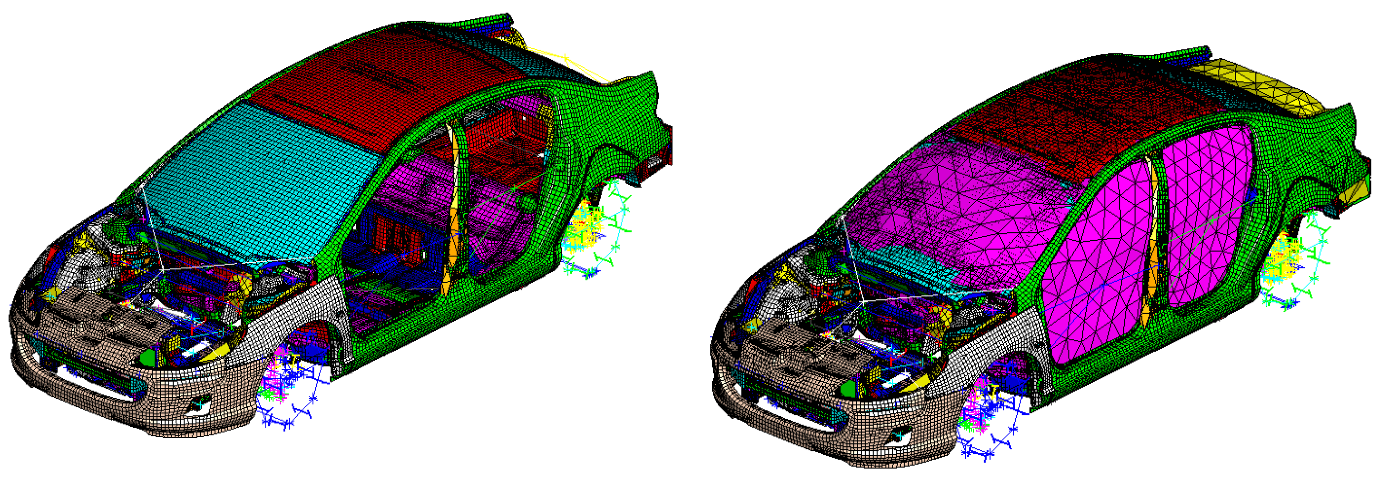
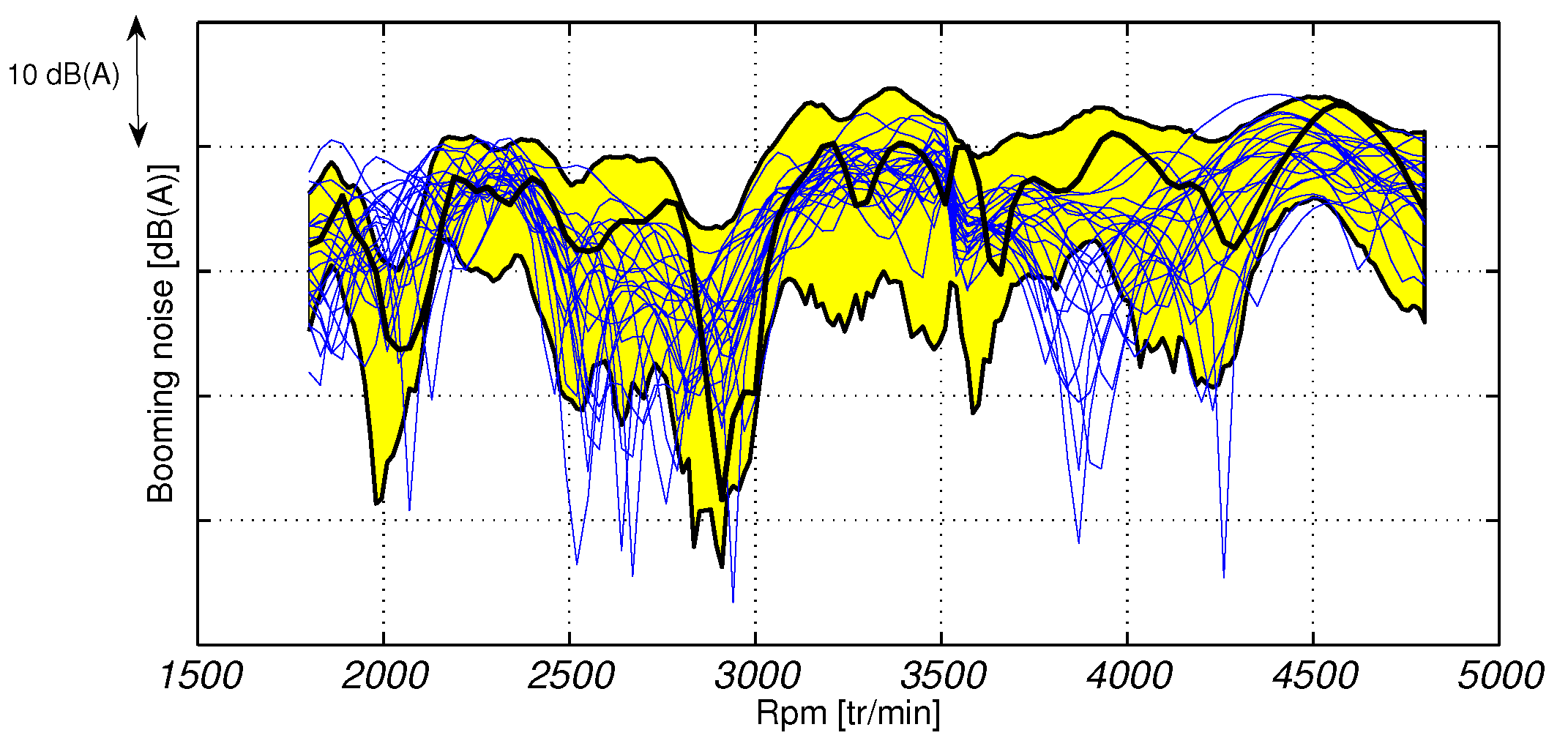
10. Experimental Validation with a Complex Computational Vibroacoustic Model of an Automobile

We present an experimental validation of the nonparametric probabilistic approach of uncertainties for a complex computational vibroacoustic model of an automobile [75,110].

Description of the vibroacoustic system. The vibroacoustic system is an automobile of a given type with several optional extra, for which a single mean computational model is developed. The experimental variabilities are due to the manufacturing process and to the optional extra. The objective is to predict the booming noise for which the engine rotation is $[1500,4800]$ rpm (rotations per minute), corresponding to the frequency band [50, 160] Hz, for which the input forces are applied to the engine supports, and for which the output observation is the acoustic pressure at a given point localized in the acoustic cavity.

Nominal computational model and stochastic reduced-order model. The nominal computational model is a finite element model of the structure and of the acoustic cavity shown in Figure 2. The structure is modeled with $978,733$ structural DOFs of displacement, and the acoustic cavity is modeled with 8139 acoustical DOFs of pressure. The structural reduced-order basis is such that $N=1722$ and the acoustical reduced-order basis is such that $N_f=57$. The hyperparameters of the stochastic reduced-order model are $\delta =({\delta }_M,{\delta }_D,{\delta }_K)$ for the structure, ${\delta }_f={\delta }_{M_f}={\delta }_{D_f}={\delta }_{K_f}$ for the acoustic cavity, and ${\delta }_C$ for the vibroacoustic coupling.

Figure 2. Finite element model of the structure (left figure). Finite element mesh of the vibroacoustic computational model (right figure). Figure from [110].

Experimental identification of hyperparameter ${\delta }_f$. The acoustical input is an acoustic source placed inside the acoustic cavity. The acoustical measurements have been performed for $\nu =30$ cars of the same type with different configurations corresponding to different seat positions, different internal temperatures, and different numbers of passengers. The acoustical pressures have been measured with ${\nu }_m=32$ microphones distributed inside the acoustic cavity. For the statistical inverse problem that is required for performing the experimental identification of hyperparameter ${\delta }_f$, the observation is the real-valued random variable U defined by

$$U={\int }_{\mathcal{B}}\mathrm{dB}(\omega )d\omega ,\mathrm{dB}(\omega )=10{log}_{10}\left\{\frac{1}{p_{\mathrm{ref}}^2}\frac{1}{{\nu }_m}\sum _{j=1}^{{\nu }_m}{|P_{k_j}(\omega )|}^2\right\},$$

(99)

in which $P_{k_1}(\omega ),\dots ,P_{k_{{\nu }_m}}(\omega )$ are the components of $\mathbf{P}(\omega )$, which correspond to the observed DOFs, and which are computed with the SROM defined by Equations (64)–(69). Let $u^{\exp ,1},\dots ,u^{\exp ,\nu }$ be the corresponding measurements for the $\nu =30$ cars. The identification of hyperparameter ${\delta }_f$ is performed by using the maximum likelihood method [87],

$${\delta }_f^{\mathrm{opt}}=arg\underset{{\delta }_f}{max}\mathcal{L}({\delta }_f),\mathcal{L}({\delta }_f)=\sum _{\ell =1}^{\nu }{log}_{10}(p_U(u^{\exp ,\ell };{\delta }_f)).$$

(100)

For $\ell =1,\dots ,\nu$, the value $p_U(u^{\exp ,\ell };{\delta }_f)$ of the probability density function (pdf) of the random variable U is estimated with the kernel density estimation method by using the SROM for which the stochastic solver has been chosen as the Monte Carlo method with ${\nu }_s=2,000$ realizations.

Experimental identification of hyperparameter $\delta =({\delta }_{M_s},{\delta }_{D_s},{\delta }_{K_s})$. The structural inputs are forces applied to the engine supports. The measurements of the accelerations in the structure have been performed for $\nu =20$ cars of the same type. The random vector-valued observation is $\mathbf{U}(\omega )=(U_1(\omega ),\dots ,U_6(\omega ))$ such that

$$U_j(\omega )={log}_{10}({\omega }^2|Y_{k_j}(\omega )|),j=1,\dots ,6,$$

(101)

in which $Y_{k_1}(\omega ),\dots ,Y_{k_6}(\omega )$ are the six components of $\mathbf{Y}(\omega )$ which correspond to the observed structural DOFs, and which are computed with the SROM defined by Equations (64)–(69). Let ${\mathbf{u}}^{\exp ,1},\dots ,{\mathbf{u}}^{\exp ,\nu }$ be the corresponding measurements for the $\nu$ cars. The identification of the hyperparameter $\delta =({\delta }_{M_s},{\delta }_{D_s},{\delta }_{K_s})$ has been performed by using the least-square method. The Monte Carlo method has been used as the stochastic solver with ${\nu }_s=1000$ realizations.

Experimental validation. The hyperparameters are fixed to their identified values, ${\delta }_f={\delta }_f^{\mathrm{opt}}$ and $\delta ={\delta }^{\mathrm{opt}}$, while ${\delta }_C$ is fixed to a given value. The SROM defined by Equations (64)–(69) is solved by using the Monte Carlo method with ${\nu }_s=600$ realizations. The prediction—with the identified SROM—of the confidence region of the internal noise at a given point of observation due to the engine excitation is displayed in Figure 3. It can be seen that this prediction is good for representing the great variabilities of the measurements, while the response given by the ROM (the nominal computational model) gives only a rough idea of the real system.

Figure 3. The horizontal axis is the engine rotation expressed in rotations per minute corresponding to the frequency band $[50,160]$ Hz. The vertical axis is the level of the acoustic pressure in dB(A). Experimental measurements (20 blue thin lines). Prediction with the ROM (black thick line). Prediction with the identified SROM of the confidence region corresponding to the probability level $0.95$ (region in yellow color of in gray). Figure from [110].

11. Conclusions

We have presented a computational methodology that is adapted to the vibroacoustics predictions of complex industrial systems in the low- and medium-frequency bands. The vibroacoustic system is made up of a dissipative structure (possibly with a viscoelastic behavior), coupled with a bounded acoustic cavity filled with a dissipative acoustic fluid, and coupled with an acoustic fluid occupying an unbounded external domain. We have presented a reduced-order computational model that is efficient for an acoustic cavity which is filled with a liquid or a gas. For the medium-frequency band, the uncertainty quantification is particularly important. For complex industrial vibroacoustic systems, the main source of uncertainties is due to modeling errors. We have summarized the nonparametric probabilistic approach of model uncertainties, and we have detailed the construction of the random matrices for the case of a viscoelastic structure in order to respect the causality of the physical system. Finally, the application to a real automobile with experimental comparisons was presented.

Appendix A.1. Linear Viscoelastic Constitutive Equation in the Frequency Domain

The general theory of linear viscoelasticity is used (see [112,113,114]). With respect to the presentation detailed in [41], we present here a summary of those results with additional developments. In this section, $\mathbf{x}$ is fixed in ${\mathsf{\Omega }}_S$ and will be omitted in all the quantities. The Latin indices, such as i, j, k, and h, take the values 1, 2, and 3. The convention for summations over repeated Latin indices is used. The general constitutive equation in the frequency range is written as

$${\sigma }_{ij}(\omega )=(a_{ijkh}(\omega )+i\omega b_{ijkh}(\omega )){\epsilon }_{kh}(\omega ).$$

(A1)

It can be proven that

$$\underset{|\omega |\to +\infty }{lim}{a}_{ijkh}(\omega )=a_{ijkh}(+\infty ),$$

(A2)

$$\underset{|\omega |\to +\infty }{lim}\omega b_{ijkh}(\omega )=0,$$

(A3)

in which $a_{ijkh}(+\infty )$ is called the initial elasticity tensor. It can be deduced that

$${\sigma }_{ij}(\infty )=a_{ijkh}(+\infty ){\epsilon }_{kh}(\infty ).$$

(A4)

Equation (A4) shows that viscoelastic materials behave elastically at high frequencies with elasticity coefficients defined by the initial elasticity tensor $a_{ijkh}(+\infty )$ that differs from the equilibrium modulus tensor $a_{ijkh}(0)$ that is such that

$${\sigma }_{ijkh}(0)=a_{ijkh}(0){\epsilon }_{ijkh}(0),$$

(A5)

in which ${\sigma }_{ijkh}(0)={\{{\sigma }_{ijkh}(\omega )\}}_{\omega =0}$ and ${\epsilon }_{ijkh}(0)={\{{\epsilon }_{ijkh}(\omega )\}}_{\omega =0}$. The reader should be aware of the fact that the constitutive equation of an elastic material in a static deformation process is defined by equilibrium modulus tensor $a_{ijkh}(0)$, and not by the initial elasticity tensor $a_{ijkh}(+\infty )$. Referring to [112,115], it has been proven that $a_{ijkh}(0)-a_{ijkh}(+\infty )$ is a negative-definite tensor. The tensors $a_{ijkh}(\omega )$ and $b_{ijkh}(\omega )$ are even functions:

$$a_{ijkh}(-\omega )=a_{ijkh}(\omega ),b_{ijkh}(-\omega )=b_{ijkh}(\omega ).$$

(A6)

Due to the symmetry properties of tensors ${\mathcal{G}}_{ijkh}(t)$, it can directly be deduced that tensors $a_{ijkh}(\omega )$ and $b_{ijkh}(\omega )$ must satisfy the symmetry properties

$$\begin{array}{c}{a}_{ijkh}(\omega )=a_{jikh}(\omega )=a_{ijhk}(\omega )=a_{khij}(\omega ),\end{array}$$

(A7)

$$\begin{array}{c}{b}_{ijkh}(\omega )=b_{jikh}(\omega )=b_{ijhk}(\omega )=b_{khij}(\omega ).\end{array}$$

(A8)

In addition, the following positive-definiteness properties can be shown. For all second-order real symmetric tensors $X_{ij}$,

$$\begin{array}{c}{a}_{ijkh}(\omega )X_{kh}{X}_{ij}\ge c_a(\omega )X_{ij}{X}_{ij},\end{array}$$

(A9)

$$\begin{array}{c}{b}_{ijkh}(\omega )X_{kh}{X}_{ij}\ge c_b(\omega )X_{ij}{X}_{ij},\end{array}$$

(A10)

in which the positive constants $c_a(\omega )$ and $c_b(\omega )$ are such that $c_a(\omega )\ge c_0>0$ and $c_b(\omega )\ge c_0>0$, where $c_0$ is a positive real constant independent of $\omega$.

Appendix A.2. Compatibility Equation between a ijkh and b ijkh

We recall that $a_{ijkh}(0)$ is the equilibrium modulus tensor that is the elastic tensor and which is denoted by $a_{ijkh}^{\mathrm{elas}}$,

$$a_{ijkh}^{\mathrm{elas}}=a_{ijkh}(0).$$

(A11)

Due to the causality property in the time domain and using the Hilbert transform for causal function [102,116,117,118,119]), it can be proven that there is a compatibility equation between $a_{ijkh}$ and $b_{ijkh}$, also called the Kramers and Kronig relation (see [120,121]), which is written

$$a_{ijkh}(\omega )=a_{ijkh}^{\mathrm{elas}}+\frac{\omega }{\pi }\mathrm{p}.\mathrm{v}{\int }_{-\infty }^{+\infty }\frac{b_{ijkh}({\omega }^{\prime })}{\omega -{\omega }^{\prime }}d{\omega }^{\prime },$$

(A12)

in which p.v denotes the Cauchy principal value. If $y\mapsto h(y)$ is a locally integrable function on the real line except in a singular point $y=0$, then the p.v is defined as

$$\mathrm{p}.\mathrm{v}{\int }_{-\infty }^{+\infty }h(y)dy=\underset{\ell \to +\infty ,\eta \to 0^{+}}{lim}\{{\int }_{-\ell }^{-\eta }h(y)dy+{\int }_{\eta }^{\ell }h(y)dy\}.$$

(A13)

Appendix A.3. Construction of the Linear Viscoelastic Constitutive Equation in the Frequency Domain

Two cases are considered.

• (i) Particular case. A family of linear viscoelastic constitutive equations can be constructed in the time domain using linear differential equations in $\sigma (t)$ and $\epsilon (t)$. The associated frequency-dependent coefficients $a_{ijkh}(\omega )$ and $b_{ijkh}(\omega )$ automatically verified Equation (A12). In this framework, some examples for $a_{ijkh}(\omega )$ and $b_{ijkh}(\omega )$ can be found in the literature (e.g., [41,98,112,113,122,123,124,125,126,127]).
• (ii) General case. In the general case for which $a_{ijkh}(\omega )$ and $b_{ijkh}(\omega )$ are not derived from such an algebraic representation but correspond to a general integral operator in the time domain (e.g., constructed using experimental curves), a rigorous method of construction is proposed below to satisfy the causality principle.

For the general case, it is assumed that a part ${\mathsf{\Omega }}_{\mathrm{visco}}$ of the structure ${\mathsf{\Omega }}_S$ is made of material modeled in the framework of the linear viscoelasticity theory (see after), while the complementary part ${\mathsf{\Omega }}_{\mathrm{damp}}$ will be modeled with a linear dissipative constitutive equation for modeling damping effects (detailed in Section A.4). We then have ${\mathsf{\Omega }}_S={\mathsf{\Omega }}_{\mathrm{visco}}\cup {\mathsf{\Omega }}_{\mathrm{damp}}$.

For the practical construction of the constitutive equation related to ${\mathsf{\Omega }}_{\mathrm{visco}}$, it is assumed that functions $\omega \mapsto b_{ijkh}(\mathbf{x},\omega )$ for $\omega \ge 0$ and equilibrium modulus tensor $a_{ijkh}^{\mathrm{elas}}(\mathbf{x})$ (which is the symmetric and positive-definite elastic tensor) are given. For real $\omega$ and for $\mathbf{x}$ belonging to ${\mathsf{\Omega }}_{\mathrm{visco}}$, functions $\omega \mapsto a_{ijkh}(\mathbf{x},\omega )$ can then be constructed.

• The given functions $\omega \mapsto b_{ijkh}(\mathbf{x},\omega )$ cannot be arbitrarily chosen, but must satisfy some hypotheses to ensure the coherence of the viscoelastic model:
  (1) For all fixed $\mathbf{x}$ and $\omega$, the tensor ${\{b_{ijkh}(\mathbf{x},\omega )\}}_{ijkh}$ must be symmetric and positive definite.
  (2) For $\omega \to +\infty$, Equation (A3) must hold, which means that functions $b_{ijkh}(\mathbf{x},\omega )$ decrease at infinity at least in ${\omega }^{-\alpha }$ with $\alpha >1$.
  (3) Functions $\omega \mapsto b_{ijkh}(\mathbf{x},\omega )$ that satisfy (1) and (2) are then extended to $\omega <0$ using the even property defined by Equation (A6).
• For all fixed $\mathbf{x}$ and $\omega$, the tensor ${\{a_{ijkh}(\mathbf{x},\omega )\}}_{ijkh}$ must be symmetric and positive definite. For all $\omega \ge 0$, functions $\omega \mapsto a_{ijkh}(\mathbf{x},\omega )$ are then constructed using the following equation (see Equation (A12)),

  $$a_{ijkh}(\mathbf{x},\omega )=a_{ijkh}^{\mathrm{elas}}(\mathbf{x})+\frac{\omega }{\pi }\mathrm{p}.\mathrm{v}{\int }_{-\infty }^{+\infty }\frac{b_{ijkh}(\mathbf{x},{\omega }^{\prime })}{\omega -{\omega }^{\prime }}d{\omega }^{\prime },$$

  (A14)

  and are extended to $\omega <0$ using the even property.
• As seen above, for all fixed $\mathbf{x}$ and $\omega$, symmetric tensor ${\{a_{ijkh}(\mathbf{x},\omega )\}}_{ijkh}$ must be positive definite. This property must then be checked at the end of the construction, and if it is not satisfied, functions $\omega \mapsto b_{ijkh}(\mathbf{x},\omega )$ must be modified. In [101], it has been shown that the following sufficient condition allows this property to be satisfied: if functions $\omega \mapsto b_{ijkh}(\mathbf{x},\omega )$ are decreasing functions for $\omega \ge 0$, then the property is verified.

Appendix A.4. Linear Dissipative Constitutive Equation for Modeling Damping Effects

This section deals with the linear dissipative constitutive equation for modeling damping effects in the part ${\mathsf{\Omega }}_{\mathrm{damp}}$ of the structure ${\mathsf{\Omega }}_S$. Several models of dissipative constitutive equation (with frequency-dependent coefficients) corresponding to an elastic material are considered for which the mechanical damping is arbitrarily introduced in order to represent damping effects. The first model presented is the constitutive equation for an elastic material with a linear viscous damping term. The second one is a constitutive equation for an elastic material with a parameterized family of damping models depending on frequency. The construction proposed for these two models is such that the causality principle will be verified, and consequently, the fourth-order tensor $a_{ijkh}(\omega )$ will depend on $\omega$ although the elastic tensor $a_{ijkh}^{\mathrm{elas}}$ of the elastic material is independent of $\omega$.

(i) Constitutive equation for an elastic material with a linear viscous damping term. In this case, the constitutive equation is given by Equation (A1), in which

$$a_{ijkh}(\mathbf{x},\omega )=a_{ijkh}^{\mathrm{elas}}(\mathbf{x}),b_{ijkh}(\mathbf{x},\omega )=b_{ijkh}(\mathbf{x}),$$

(A15)

in which the tensors $a_{ijkh}^{\mathrm{elas}}(\mathbf{x})$ and $b_{ijkh}(\mathbf{x})$ are symmetric positive definite and independent of $\omega$.

(ii) Constitutive equation for an elastic material with a parameterized family of damping models depending on frequency. The constitutive equation is then defined as an elastic material with a parameterized family of damping models depending on frequency and is written as

$$b_{ijkh}(\mathbf{x},\omega )=\chi (\omega )a_{ijkh}^{\mathrm{elas}}(\mathbf{x}),$$

(A16)

in which the tensor $a_{ijkh}^{\mathrm{elas}}(\mathbf{x})$ is symmetric positive definite and where $\chi (\omega )$ is a positive-valued real function in $\omega$ which must satisfy the following properties:

(1)

For $\omega \to +\infty$, function $\chi (\omega )$ must decrease at infinity at least in ${\omega }^{-\alpha }$ in which $\alpha >1$.

(2)

Function $\chi$ is even, $\chi (-\omega )=\chi (\omega )$.

From Equation (A14), it can be deduced that for all fixed $\mathbf{x}$ and for all $\omega \ge 0$, the symmetric positive definite tensor must be constructed by the following equation:

$$a_{ijkh}(\mathbf{x},\omega )=\left\{1+\frac{\omega }{\pi }\mathrm{p}.\mathrm{v}{\int }_{-\infty }^{+\infty }\frac{\chi ({\omega }^{\prime })}{\omega -{\omega }^{\prime }}d{\omega }^{\prime }\right\}{a}_{ijkh}^{\mathrm{elas}}(\mathbf{x}),$$

(A17)

in order to ensure the causality property for the constitutive equation. For $\omega <0$, the values of $a_{ijkh}(\mathbf{x},\omega )$ are obtained using the even property in $\omega$ of functions $a_{ijkh}(\mathbf{x},\omega )$. Finally, function $\chi (\omega )$ must be such that for all fixed $\mathbf{x}$ and $\omega$, symmetric tensor ${\{a_{ijkh}(\mathbf{x},\omega )\}}_{ijkh}$ is positive definite. As previously explained, this property will be satisfied if function $\chi (\omega )$ is a decreasing function for $\omega \ge 0$.

Appendix B.1. Exterior Neumann Boundary Value Problem Related to the Helmholtz Equation

The geometry is defined in Figure A1. The equations of the exterior Neumann problem related to the Helmholtz equation (see Equations (1)–(3)) are rewritten in terms of a velocity potential $\psi (\mathbf{x},\omega )$. Let $\mathbf{v}(\mathbf{x},\omega )=\mathbf{\nabla }\psi (\mathbf{x},\omega )$ be the velocity field of the fluid. The acoustic pressure $p(\mathbf{x},\omega )$ is related to $\psi (\mathbf{x},\omega )$ by the following equation:

$$p(\mathbf{x},\omega )=-i\omega {\rho }_{\mathrm{E}}\psi (\mathbf{x},\omega )\mathrm{in}{\mathsf{\Omega }}_E,$$

(A18)

where ${\rho }_{\mathrm{E}}$ is the constant mass density of the external fluid at equilibrium. Let $c_{\mathrm{E}}$ be the constant speed of sound in the external fluid at equilibrium, and let $k=\omega /c_{\mathrm{E}}$ be the wave number at frequency $\omega$. The exterior Neumann problem is written as

$${\mathbf{\nabla }}^2\psi (\mathbf{x},\omega )+k^2\psi (\mathbf{x},\omega )=0\mathrm{in}{\mathsf{\Omega }}_E,$$

(A19)

$$\frac{\partial \psi (\mathbf{y},\omega )}{\partial {\mathbf{n}}_{\mathbf{y}}}=v(\mathbf{y})\mathrm{on}{\mathsf{\Gamma }}_E,$$

(A20)

$$|\psi |=O(\frac{1}{R}),\left|\frac{\partial \psi }{\partial R}+ik\psi \right|=O(\frac{1}{R^2}),$$

(A21)

with $R=\parallel \mathbf{x}\parallel \to +\infty$, where $\partial /\partial R$ is the derivative in the radial direction and where $v(\mathbf{y})$ is the given normal velocity field on ${\mathsf{\Gamma }}_E$. Equation (A19) is the Helmholtz equation in the external acoustic fluid, Equation (A20) is the Neumann condition on external fluid–structure interface ${\mathsf{\Gamma }}_E$, and Equation (A21) corresponds to the outward Sommerfeld radiation condition at infinity. For arbitrary real $\omega \ne 0$, the boundary value problem defined by Equations (A19)–(A21) admits a unique solution denoted ${\psi }^{\mathrm{sol}}$ that depends linearly on the normal velocity v [97,98].

Appendix B.2. Introduction of the Acoustic Impedance Boundary Operator and Radiation Impedance Operator

Let ${\psi }_{{\mathsf{\Gamma }}_{{}_E}}^{\mathrm{sol}}$ be the value of ${\psi }^{\mathrm{sol}}$ on ${\mathsf{\Gamma }}_E$. For all $\mathbf{x}$ in ${\mathsf{\Omega }}_E$, let $\mathbf{R}(\mathbf{x},\omega /c_{\mathrm{E}})$ be the complex linear operator such that

$${\psi }^{\mathrm{sol}}(\mathbf{x},\omega )=\mathbf{R}(\mathbf{x},\omega /c_{\mathrm{E}})v,$$

(A22)

and let ${\mathbf{B}}_{{\mathsf{\Gamma }}_E}(\omega /c_{\mathrm{E}})$ be the complex linear boundary operator such that

$${\psi }_{{}_{{\mathsf{\Gamma }}_{{}_E}}}^{\mathrm{sol}}={\mathbf{B}}_{{\mathsf{\Gamma }}_E}(\omega /c_{\mathrm{E}})v.$$

(A23)

Using Equation (A18), for all $\mathbf{x}$ in ${\mathsf{\Omega }}_E$, the pressure field $p(\mathbf{x},\omega )$ is written as

$$p(\mathbf{x},\omega )={\mathbf{Z}}_{\mathrm{rad}}(\mathbf{x},\omega )v,$$

(A24)

in which ${\mathbf{Z}}_{\mathrm{rad}}(\mathbf{x},\omega )$ is called the radiation impedance operator that can then be written as

$${\mathbf{Z}}_{\mathrm{rad}}(\mathbf{x},\omega )=-i\omega {\rho }_{\mathrm{E}}\mathbf{R}(\mathbf{x},\omega /c_{\mathrm{E}}).$$

(A25)

Similarly, the pressure field ${p|}_{{\mathsf{\Gamma }}_E}(\omega )$ on ${\mathsf{\Gamma }}_E$ is written as

$${p|}_{{}_{{\mathsf{\Gamma }}_E}}(\omega )={\mathbf{Z}}_{{\mathsf{\Gamma }}_E}(\omega )v,$$

(A26)

in which ${\mathbf{Z}}_{{\mathsf{\Gamma }}_E}(\omega )$ is called the acoustic impedance boundary operator, which can then be written as

$${\mathbf{Z}}_{{\mathsf{\Gamma }}_E}(\omega )=-i\omega {\rho }_{\mathrm{E}}{\mathbf{B}}_{{\mathsf{\Gamma }}_E}(\omega /c_{\mathrm{E}}).$$

(A27)

Appendix B.3. Algebraic Properties of the Acoustic Impedance Boundary Operator

Let ${}^t{\mathbf{B}}_{{\mathsf{\Gamma }}_E}(\omega /c_{\mathrm{E}})$ be the transpose of complex operator ${\mathbf{B}}_{{\mathsf{\Gamma }}_E}(\omega /c_{\mathrm{E}})$. We have the following symmetry property:

$${}^t{\mathbf{B}}_{{\mathsf{\Gamma }}_E}(\omega /c_{\mathrm{E}})={\mathbf{B}}_{{\mathsf{\Gamma }}_E}(\omega /c_{\mathrm{E}}),$$

(A28)

and from Equation (A27), it can be deduced that

$${}^t{\mathbf{Z}}_{{\mathsf{\Gamma }}_E}(\omega )={\mathbf{Z}}_{{\mathsf{\Gamma }}_E}(\omega ).$$

(A29)

It should be noted that these complex operators are symmetric but not Hermitian. Operator $i\omega {\mathbf{Z}}_{{\mathsf{\Gamma }}_E}(\omega )$ can be written as

$$i\omega {\mathbf{Z}}_{{\mathsf{\Gamma }}_E}(\omega )=-{\omega }^2{\mathbf{M}}_{{\mathsf{\Gamma }}_E}(\omega /c_{\mathrm{E}})+i\omega {\mathbf{D}}_{{\mathsf{\Gamma }}_E}(\omega /c_{\mathrm{E}}),$$

(A30)

in which ${\mathbf{M}}_{{\mathsf{\Gamma }}_E}(\omega /c_{\mathrm{E}})$ and ${\mathbf{D}}_{{\mathsf{\Gamma }}_E}(\omega /c_{\mathrm{E}})$ are two real linear operators such that

$$\omega {\mathbf{M}}_{{\mathsf{\Gamma }}_E}(\omega /c_{\mathrm{E}})=\Im m{\mathbf{Z}}_{{\mathsf{\Gamma }}_E}(\omega ),$$

(A31)

$${\mathbf{D}}_{{\mathsf{\Gamma }}_E}(\omega /c_{\mathrm{E}})=\Re e{\mathbf{Z}}_{{\mathsf{\Gamma }}_E}(\omega ).$$

(A32)

The real part ${\mathbf{D}}_{{\mathsf{\Gamma }}_E}(\omega /c_{\mathrm{E}})$ of the acoustic impedance boundary operator is symmetric and positive, due to the Sommerfeld radiation condition at infinity.

Appendix B.4. Construction of the Acoustic Impedance Boundary Operator for All Real Values of the Frequency

This construction is based on the use of two boundary integral equations on ${\mathsf{\Gamma }}_E$. The first one is based on the use of a single- and double-layer potentials on ${\mathsf{\Gamma }}_E$. The second is obtained by the taking the normal derivative on ${\mathsf{\Gamma }}_E$ of the first one. We then obtained the following system relating ${\psi }_{{\mathsf{\Gamma }}_{{}_E}}^{\mathrm{sol}}$ to v, which then allows ${\mathbf{B}}_{{\mathsf{\Gamma }}_E}(\omega /c_{\mathrm{E}})$ to be defined using Equation (A23),

$$\left[\begin{array}{c}0\\ \mathbf{I}{\psi }_{{}_{{\mathsf{\Gamma }}_{{}_E}}}^{\mathrm{sol}}\end{array}\right]=\left[\begin{array}{cc}-{\mathbf{S}}_{\mathrm{T}}(\omega /c_{\mathrm{E}})& \frac{1}{2}{}^t\mathbf{I}-{}^t{\mathbf{S}}_{\mathrm{D}}(\omega /c_{\mathrm{E}})\\ \frac{1}{2}\mathbf{I}-{\mathbf{S}}_{\mathrm{D}}(\omega /c_{\mathrm{E}})& {\mathbf{S}}_{\mathrm{S}}(\omega /c_{\mathrm{E}})\end{array}\right]\left[\begin{array}{c}{\psi }_{{}_{{\mathsf{\Gamma }}_{{}_E}}}\\ v\end{array}\right].$$

(A33)

The linear boundary integral operators ${\mathbf{S}}_{\mathrm{S}}(\omega /c_{\mathrm{E}})$, ${\mathbf{S}}_{\mathrm{D}}(\omega /c_{\mathrm{E}})$, and ${\mathbf{S}}_{\mathrm{T}}(\omega /c_{\mathrm{E}})$ are defined by

$$<{\mathbf{S}}_{\mathrm{S}}(\omega /c_{\mathrm{E}})v,\delta v>={\int }_{{\mathsf{\Gamma }}_E}{\int }_{{\mathsf{\Gamma }}_E}G(\mathbf{x}-\mathbf{y})v(\mathbf{y})\delta v(\mathbf{x})d{s}_{\mathbf{y}}d{s}_{\mathbf{x}},$$

(A34)

$$<{\mathbf{S}}_{\mathrm{D}}(\omega /c_{\mathrm{E}}){\psi }_{{}_{{\mathsf{\Gamma }}_{{}_E}}},\delta v>={\int }_{{\mathsf{\Gamma }}_E}{\int }_{{\mathsf{\Gamma }}_E}\frac{\partial G(\mathbf{x}-\mathbf{y})}{\partial {\mathbf{n}}_{\mathbf{y}}}{\psi }_{{}_{{\mathsf{\Gamma }}_{{}_E}}}(\mathbf{y})\delta v(\mathbf{x})d{s}_{\mathbf{y}}d{s}_{\mathbf{x}},$$

(A35)

$$\begin{array}{c}{\displaystyle <{\mathbf{S}}_{\mathrm{T}}(\omega /c_{\mathrm{E}}){\psi }_{{}_{{\mathsf{\Gamma }}_{{}_E}}},\delta {\psi }_{{}_{{\mathsf{\Gamma }}_{{}_E}}}>=-k^2{\int }_{{\mathsf{\Gamma }}_E}{\int }_{{\mathsf{\Gamma }}_E}G(\mathbf{x}-\mathbf{y}){\mathbf{n}}_{\mathbf{x}}·{\mathbf{n}}_{\mathbf{y}}{\psi }_{{}_{{\mathsf{\Gamma }}_{{}_E}}}(\mathbf{y})\delta {\psi }_{{}_{{\mathsf{\Gamma }}_{{}_E}}}(\mathbf{x})d{s}_{\mathbf{y}}d{s}_{\mathbf{x}}}\\ +{\int }_{{\mathsf{\Gamma }}_E}{\int }_{{\mathsf{\Gamma }}_E}G(\mathbf{x}-\mathbf{y})\{{\mathbf{n}}_{\mathbf{y}}\times {\mathbf{\nabla }}_{\mathbf{y}}{\psi }_{{}_{{\mathsf{\Gamma }}_{{}_E}}}(\mathbf{y})\}·\{{\mathbf{n}}_{\mathbf{x}}\times {\mathbf{\nabla }}_{\mathbf{x}}\delta {\psi }_{{}_{{\mathsf{\Gamma }}_{{}_E}}}(\mathbf{x})\}d{s}_{\mathbf{y}}d{s}_{\mathbf{x}},\end{array}$$

(A36)

where $G(\mathbf{x}-\mathbf{y})$ is the Green function, which is written as

$$G(\mathbf{x}-\mathbf{y})=g(\parallel \mathbf{x}-\mathbf{y}\parallel )=-{(4\pi )}^{-1}{e}^{-ikr}/r,$$

(A37)

in which $r=\parallel \mathbf{x}-\mathbf{y}\parallel$. In Equations (A34)–(A36), the brackets correspond to bilinear forms which allow the operators to be defined, and the functions $\delta v$ and $\delta {\psi }_{{\mathsf{\Gamma }}_{{}_E}}$ are associated with functions v and ${\psi }_{{\mathsf{\Gamma }}_{{}_E}}$. Considering Equation (A33), let $\mathbf{H}(\omega /c_{\mathrm{E}})$ be the operator defined by

$$\mathbf{H}(\omega /c_{\mathrm{E}})=\left[\begin{array}{cc}-{\mathbf{S}}_{\mathrm{T}}(\omega /c_{\mathrm{E}})& \frac{1}{2}{}^t\mathbf{I}-{}^t{\mathbf{S}}_{\mathrm{D}}(\omega /c_{\mathrm{E}})\\ \frac{1}{2}\mathbf{I}-{\mathbf{S}}_{\mathrm{D}}(\omega /c_{\mathrm{E}})& {\mathbf{S}}_{\mathrm{S}}(\omega /c_{\mathrm{E}})\end{array}\right].$$

(A38)

Operator $\mathbf{H}(\omega /c_{\mathrm{E}})$ has the symmetric property, ${}^t\mathbf{H}(\omega /c_{\mathrm{E}})=\mathbf{H}(\omega /c_{\mathrm{E}})$. In Equation (A33), the first equation can be rewritten as ${\mathbf{S}}_{\mathrm{T}}(\omega /c_{\mathrm{E}}){\psi }_{{\mathsf{\Gamma }}_{{}_E}}=(\frac{1}{2}{}^t\mathbf{I}-{}^t{\mathbf{S}}_{\mathrm{D}}(\omega /c_{\mathrm{E}}))v$. This classical boundary equation that allows the velocity potential to be calculated for a given normal velocity has a unique solution for all real $\omega$, which does not belong to the set of frequencies for which ${\mathbf{S}}_{\mathrm{T}}(\omega /c_{\mathrm{E}})$ has a null space that is not reduced to $\{0\}$. This set of frequencies is called the set of spurious frequencies. Consequently, for a frequency that is a spurious frequency, ${\psi }_{{\mathsf{\Gamma }}_{{}_E}}$ is the sum of solution ${\psi }_{{\mathsf{\Gamma }}_{{}_E}}^{\mathrm{sol}}$ with an arbitrary element of the null space of ${\mathbf{S}}_{\mathrm{T}}(\omega /c_{\mathrm{E}})$. The method then consists of using the second equation that is written as ${\psi }_{{\mathsf{\Gamma }}_{{}_E}}^{\mathrm{sol}}=(\frac{1}{2}\mathbf{I}-{\mathbf{S}}_{\mathrm{D}}(\omega /c_{\mathrm{E}})){\psi }_{{\mathsf{\Gamma }}_{{}_E}}+{\mathbf{S}}_{\mathrm{S}}(\omega /c_{\mathrm{E}})v$, and which yields solution ${\psi }_{{\mathsf{\Gamma }}_{{}_E}}^{\mathrm{sol}}$ for all real $\omega$. Concerning the practical construction of ${\psi }_{{\mathsf{\Gamma }}_{{}_E}}^{\mathrm{sol}}$, for all real values of $\omega$, using Equation (A33), a particular elimination procedure is described in Section B.6.

Appendix B.5. Construction of the Radiation Impedance Operator

The solution $\{{\psi }^{\mathrm{sol}}(\mathbf{x},\omega ),\mathbf{x}\in {\mathsf{\Omega }}_E\}$ of Equations (A19)–(A21) can be calculated using the following integral equation:

$${\psi }^{\mathrm{sol}}(\mathbf{x},\omega )={\int }_{{\mathsf{\Gamma }}_E}\{G(\mathbf{x}-\mathbf{y})v(\mathbf{y})-{\psi }_{{}_{{\mathsf{\Gamma }}_{{}_E}}}^{\mathrm{sol}}(\mathbf{y},\omega )\frac{\partial G(\mathbf{x}-\mathbf{y})}{\partial {\mathbf{n}}_{\mathbf{y}}}\}d{s}_{\mathbf{y}}.$$

(A39)

For all $\mathbf{x}$ fixed in ${\mathsf{\Omega }}_E$, the linear integral operators ${\mathbf{R}}_{\mathrm{S}}(\mathbf{x},\omega /c_{\mathrm{E}})$ and ${\mathbf{R}}_{\mathrm{D}}(\mathbf{x},\omega /c_{\mathrm{E}})$ are defined by

$${\mathbf{R}}_{\mathrm{S}}(\mathbf{x},\omega /c_{\mathrm{E}})v={\int }_{{\mathsf{\Gamma }}_E}G(\mathbf{x}-\mathbf{y})v(\mathbf{y})d{s}_{\mathbf{y}},$$

(A40)

$${\mathbf{R}}_{\mathrm{D}}(\mathbf{x},\omega /c_{\mathrm{E}}){\psi }_{{}_{{\mathsf{\Gamma }}_{{}_E}}}={\int }_{{\mathsf{\Gamma }}_E}{\psi }_{{}_{{\mathsf{\Gamma }}_{{}_E}}}(\mathbf{y})\frac{\partial G(\mathbf{x}-\mathbf{y})}{\partial {\mathbf{n}}_{\mathbf{y}}}d{s}_{\mathbf{y}}.$$

(A41)

Using Equation (A23), Equation (A39) can be rewritten as

$${\psi }^{\mathrm{sol}}(\mathbf{x},\omega )=\{{\mathbf{R}}_{\mathrm{S}}(\mathbf{x},\omega /c_{\mathrm{E}})-{\mathbf{R}}_{\mathrm{D}}(\mathbf{x},\omega /c_{\mathrm{E}}){\mathbf{B}}_{{\mathsf{\Gamma }}_E}(\omega /c_{\mathrm{E}})\}v.$$

(A42)

From Equation (A22), it can be deduced that, for all $\mathbf{x}$ in ${\mathsf{\Omega }}_E$,

$$\mathbf{R}(\mathbf{x},\omega /c_{\mathrm{E}})={\mathbf{R}}_{\mathrm{S}}(\mathbf{x},\omega /c_{\mathrm{E}})-{\mathbf{R}}_{\mathrm{D}}(\mathbf{x},\omega /c_{\mathrm{E}}){\mathbf{B}}_{{\mathsf{\Gamma }}_E}(\omega /c_{\mathrm{E}}),$$

(A43)

and the radiation impedance operator ${\mathbf{Z}}_{\mathrm{rad}}(\mathbf{x},\omega )$ is derived from Equations (A25) and (A43),

$${\mathbf{Z}}_{\mathrm{rad}}(\mathbf{x},\omega )=-i\omega {\rho }_{\mathrm{E}}\{{\mathbf{R}}_{\mathrm{S}}(\mathbf{x},\omega /c_{\mathrm{E}})-{\mathbf{R}}_{\mathrm{D}}(\mathbf{x},\omega /c_{\mathrm{E}}){\mathbf{B}}_{{\mathsf{\Gamma }}_E}(\omega /c_{\mathrm{E}})\}.$$

(A44)

Appendix B.6. Symmetric Boundary Element Method without Spurious Frequencies

The finite element method is used for discretizing the boundary integral operators ${\mathbf{S}}_{\mathrm{S}}(\omega /c_{\mathrm{E}})$, ${\mathbf{S}}_{\mathrm{D}}(\omega /c_{\mathrm{E}})$, and ${\mathbf{S}}_{\mathrm{T}}(\omega /c_{\mathrm{E}})$ (called a boundary element method). Let us consider a finite element mesh of boundary ${\mathsf{\Gamma }}_E$. Let $\mathbf{V}=(V_1,\dots ,V_{n_E})$ and ${\mathsf{\Psi }}_{{\mathsf{\Gamma }}_{{}_E}}=({\mathsf{\Psi }}_{{\mathsf{\Gamma }}_{{}_E},1},\dots ,{\mathsf{\Psi }}_{{\mathsf{\Gamma }}_{{}_E},n_E})$ be the complex vectors of the $n_E$ degrees-of-freedom consisting of the values of v and ${\psi }_{{\mathsf{\Gamma }}_{{}_E}}$ at the nodes of the mesh. Let $[S_{\mathrm{S}}(\omega /c_{\mathrm{E}})]$, $[S_{\mathrm{D}}(\omega /c_{\mathrm{E}})]$, and $[S_{\mathrm{T}}(\omega /c_{\mathrm{E}})]$ be the full complex matrices corresponding to the discretization of the operators defined in Equations (A34)–(A36). The complex matrices $[S_{\mathrm{S}}(\omega /c_{\mathrm{E}})]$ and $[S_{\mathrm{T}}(\omega /c_{\mathrm{E}})]$ are symmetric. The finite element discretization of Equation (A33) yields

$$\left[\begin{array}{c}0\\ [E]{\mathsf{\Psi }}_{{}_{{\mathsf{\Gamma }}_{{}_E}}}^{\mathrm{sol}}\end{array}\right]=[H(\omega /c_{\mathrm{E}})]\left[\begin{array}{c}{\mathsf{\Psi }}_{{}_{{\mathsf{\Gamma }}_{{}_E}}}\\ \mathbf{V}\end{array}\right],$$

(A45)

in which the symmetric complex matrix $[H(\omega /c_{\mathrm{E}})]$ is written as

$$\left[\begin{array}{cc}-[S_{\mathrm{T}}(\omega /c_{\mathrm{E}})]& \frac{1}{2}{[E]}^T-{[S_{\mathrm{D}}(\omega /c_{\mathrm{E}})]}^T\\ \frac{1}{2}[E]-[S_{\mathrm{D}}(\omega /c_{\mathrm{E}})]& [S_{\mathrm{S}}(\omega /c_{\mathrm{E}})]\end{array}\right].$$

(A46)

In Equation (A45), ${\mathsf{\Psi }}_{{\mathsf{\Gamma }}_{{}_E}}^{\mathrm{sol}}$ is the complex vector of the nodal unknowns corresponding to the finite element discretization of ${\psi }_{{\mathsf{\Gamma }}_{{}_E}}^{\mathrm{sol}}$. The matrix $[E]$ is the non-diagonal $(n_E\times n_E)$ real matrix corresponding to the discretization of identity operator $\mathbf{I}$. The elimination of ${\mathsf{\Psi }}_{{\mathsf{\Gamma }}_{{}_E}}$ in Equation (A45) yields a linear equation between $[E]{\mathsf{\Psi }}_{{\mathsf{\Gamma }}_{{}_E}}^{\mathrm{sol}}$ and $\mathbf{V}$, which defines the symmetric $(n_E\times n_E)$ complex matrix $[B_{{\mathsf{\Gamma }}_E}(\omega /c_{\mathrm{E}})]$, which corresponds to the finite element discretization of boundary integral operator ${\mathbf{B}}_{{\mathsf{\Gamma }}_E}(\omega /c_{\mathrm{E}})$,

$$[E]{\mathsf{\Psi }}_{{}_{{\mathsf{\Gamma }}_{{}_E}}}^{\mathrm{sol}}=[B_{{\mathsf{\Gamma }}_E}(\omega /c_{\mathrm{E}})]\mathbf{V}.$$

(A47)

Vector ${\mathsf{\Psi }}_{{\mathsf{\Gamma }}_{{}_E}}$ is eliminated using a Gauss elimination with a partial row pivoting algorithm [138]. If $\omega$ does not belong to the set of the spurious frequencies, then $[S_{\mathrm{T}}(\omega /c_{\mathrm{E}})]$ is invertible and the elimination in Equation (A45) is performed up to row number $n_E$. If $\omega$ coincides with a spurious frequency ${\omega }_{\alpha }$ (i.e., $\omega ={\omega }_{\alpha }$), then $[S_{\mathrm{T}}({\omega }_{\alpha }/c_{\mathrm{E}})]$ is not invertible, and its null space is a real subspace of ${\mathbb{C}}^{n_E}$ of dimension $n_{\alpha }<n_E$. In this case, the elimination in Equation (A45) is performed up to row number $n_E-n_{\alpha }$. In practice, $n_{\alpha }$ is unknown. During the Gauss elimination with a partial row pivoting algorithm, the elimination process is stopped when a “zero” pivot is encountered. It should be noted that when the elimination is stopped, the equations corresponding to row numbers $n_E-n_{\alpha }+1,\dots ,n_E$ are automatically satisfied. From Equation (A27), we deduce that the $(n_E\times n_E)$ complex symmetric matrix $[Z_{{\mathsf{\Gamma }}_E}(\omega )]$ of operator ${\mathbf{Z}}_{{\mathsf{\Gamma }}_E}(\omega )$ is such that

$$[Z_{{\mathsf{\Gamma }}_E}(\omega )]=-i\omega {\rho }_{\mathrm{E}}[B_{{\mathsf{\Gamma }}_E}(\omega /c_{\mathrm{E}})].$$

(A48)

The finite element discretization of the acoustic radiation impedance operator ${\mathbf{Z}}_{\mathrm{rad}}(\mathbf{x},\omega )$, defined by Equation (A45), is written as

$$[Z_{\mathrm{rad}}(\mathbf{x},\omega )]=-i\omega {\rho }_{\mathrm{E}}\{[R_{\mathrm{S}}(\mathbf{x},\omega /c_{\mathrm{E}})]-[R_{\mathrm{D}}(\mathbf{x},\omega /c_{\mathrm{E}})][B_{{\mathsf{\Gamma }}_E}(\omega /c_{\mathrm{E}})]\}.$$

(A49)

Appendix B.7. Acoustic Response to Prescribed Wall Displacement Field and Acoustic Source Density

We consider the acoustic response of the infinite external acoustic fluid submitted to an external acoustic excitation induced by an acoustic source $Q_E(\mathbf{x},\omega )$ and to a normal velocity field on ${\mathsf{\Gamma }}_E$, which is written as $v=i\omega \mathbf{u}(\omega )·{\mathbf{n}}^S$ (see Section 2 and Figure 1).

(i) Pressure in ${\mathsf{\Omega }}_E$. For all $\mathbf{x}$ in ${\mathsf{\Omega }}_E$, the total pressure $p_E(\mathbf{x},\omega )$ is written as

$$p_E(\mathbf{x},\omega )=p_{\mathrm{rad}}(\mathbf{x},\omega )+p_{\mathrm{given}}(\mathbf{x},\omega ).$$

(A50)

The field $p_{\mathrm{rad}}(\mathbf{x},\omega )$ that is radiated by the boundary ${\mathsf{\Gamma }}_E$ submitted to the given velocity field v is written (see Equation (A24)) as

$$p_{\mathrm{rad}}(\mathbf{x},\omega )=i\omega {\mathbf{Z}}_{\mathrm{rad}}(\mathbf{x},\omega )\{\mathbf{u}(\omega )·{\mathbf{n}}^S\}.$$

(A51)

The given pressure $p_{\mathrm{given}}(\mathbf{x},\omega )$ is such that

$$p_{\mathrm{given}}(\mathbf{x},\omega )=p_{\mathrm{inc},\mathrm{Q}}(\mathbf{x},\omega )-{\mathbf{Z}}_{\mathrm{rad}}(\mathbf{x},\omega )\{\frac{\partial {\psi }_{\mathrm{inc},\mathrm{Q}}}{\partial {\mathbf{n}}^S}\},$$

(A52)

in which $p_{\mathrm{inc},\mathrm{Q}}(\mathbf{x},\omega )$ is the pressure in the free space induced by the acoustic source $Q_E$, which is written as

$$p_{\mathrm{inc},\mathrm{Q}}(\mathbf{x},\omega )=-i\omega {\int }_{K_Q}G(\mathbf{x}-{\mathbf{x}}^{\prime })Q({\mathbf{x}}^{\prime },\omega )d{\mathbf{x}}^{\prime },$$

(A53)

where G is defined by Equation (A37), and where $\partial {\psi }_{\mathrm{inc},\mathrm{Q}}/\partial {\mathbf{n}}^S$ is deduced from Equations (A18) and (A53). In the right-hand side of Equation (A52), the second term corresponds to the scattering of the incident wave induced by the external acoustic source by the boundary ${\mathsf{\Gamma }}_E$ that is considered as rigid and fixed.

(ii) Pressure on ${\mathsf{\Gamma }}_E$. From Equation (A50), it can be deduced that the total pressure on ${\mathsf{\Gamma }}_E$ is written as

$$p_E{|}_{{}_{{\mathsf{\Gamma }}_E}}(\omega )=p_{\mathrm{rad}}{{|}_{{}_{{\mathsf{\Gamma }}_E}}(\omega )+p_{\mathrm{given}}|}_{{}_{{\mathsf{\Gamma }}_E}}(\omega ),$$

(A54)

in which $p_{\mathrm{rad}}{|}_{{\mathsf{\Gamma }}_E}(\omega )$ is such that

$$p_{\mathrm{rad}}{|}_{{}_{{\mathsf{\Gamma }}_E}}(\omega )=i\omega {\mathbf{Z}}_{{\mathsf{\Gamma }}_E}(\omega )\{\mathbf{u}(\omega )·{\mathbf{n}}^S\},$$

(A55)

and where the pressure field $p_{\mathrm{given}}{|}_{{\mathsf{\Gamma }}_E}(\omega )$ on ${\mathsf{\Gamma }}_E$ is written

$$p_{\mathrm{given}}{{|}_{{}_{{\mathsf{\Gamma }}_E}}(\omega )=p_{\mathrm{inc},\mathrm{Q}}|}_{{}_{{\mathsf{\Gamma }}_E}}(\omega )-{\mathbf{Z}}_{{\mathsf{\Gamma }}_E}(\omega )\{\frac{\partial {\psi }_{\mathrm{inc},\mathrm{Q}}}{\partial {\mathbf{n}}^S}\}.$$

(A56)

Equation (A54) can then be rewritten as

$$p_E{{|}_{{}_{{\mathsf{\Gamma }}_E}}(\omega )=p_{\mathrm{given}}|}_{{}_{{\mathsf{\Gamma }}_E}}(\omega )+i\omega {\mathbf{Z}}_{{\mathsf{\Gamma }}_E}(\omega )\{\mathbf{u}(\omega )·{\mathbf{n}}^S\}.$$

(A57)

Appendix B.8. Asymptotic Formula for the Radiated Pressure Far Field

At point $\mathbf{x}$ in the external domain ${\mathsf{\Omega }}_E$, the radiated pressure $p(\mathbf{x},\omega )$ is given (see Equation (A24)) by $p(\mathbf{x},\omega )={\mathbf{Z}}_{\mathrm{rad}}(\mathbf{x},\omega )v$. For an observation point $\mathbf{x}$ that is far from the structure, the Green function is rapidly oscillating that induces numerical difficulties for performing the integration over ${\mathsf{\Gamma }}_E$. To circumvent this difficulty, asymptotic formulas can be used. Introducing the following parameterization of vector $\mathbf{x}$ ,

$$\mathbf{x}=R\mathbf{e}\mathrm{with}R=\parallel \mathbf{x}\parallel ,$$

(A58)

the asymptotic formulas are written as

$$\underset{R\to +\infty }{lim}{\mathbf{R}}_{\mathrm{S}}(R\mathbf{e};\omega /c_{\mathrm{E}})={\mathbf{R}}_{\mathrm{S}}^{\infty }(R,\mathbf{e};\omega /c_{\mathrm{E}}),$$

(A59)

$$\underset{R\to +\infty }{lim}{\mathbf{R}}_{\mathrm{D}}(R\mathbf{e};\omega /c_{\mathrm{E}})={\mathbf{R}}_{\mathrm{D}}^{\infty }(R,\mathbf{e};\omega /c_{\mathrm{E}}),$$

(A60)

in which the operators ${\mathbf{R}}_{\mathrm{S}}^{\infty }(R,\mathbf{e};\omega /c_{\mathrm{E}})$ and ${\mathbf{R}}_{\mathrm{D}}^{\infty }(R,\mathbf{e};\omega /c_{\mathrm{E}})$ are defined by

$${\mathbf{R}}_{\mathrm{S}}^{\infty }(R,\mathbf{e};\omega /c_{\mathrm{E}})v=\frac{{}_1}{{}^R}{e}^{-i\omega R/c_{\mathrm{E}}}{\int }_{{\mathsf{\Gamma }}_E}{N}_{\mathbf{e}}(\mathbf{y})v(\mathbf{y})d{s}_{\mathbf{y}},$$

(A61)

$${\mathbf{R}}_{\mathrm{D}}^{\infty }(R,\mathbf{e};\omega /c_{\mathrm{E}}){\psi }_{{}_{{\mathsf{\Gamma }}_{{}_E}}}=\frac{i\omega }{c_{\mathrm{E}}}\frac{1}{R}{e}^{-i\omega R/c_{\mathrm{E}}}{\int }_{{\mathsf{\Gamma }}_E}\mathbf{e}·{\mathbf{n}}_{\mathbf{y}}{N}_{\mathbf{e}}(\mathbf{y}){\psi }_{{}_{{\mathsf{\Gamma }}_{{}_E}}}(\mathbf{y})d{s}_{\mathbf{y}},$$

(A62)

with

$$N_{\mathbf{e}}(\mathbf{y})=-\frac{1}{4\pi }exp(i\mathbf{e}·\mathbf{y}\omega /c_{\mathrm{E}}).$$

(A63)

From Equation (A43), the asymptotic formula for the radiation impedance operator is then written as

$$\underset{R\to +\infty }{lim}{\mathbf{Z}}_{\mathrm{rad}}(R\mathbf{e},\omega )=-i\omega {\rho }_{\mathrm{E}}\{{\mathbf{R}}_{\mathrm{S}}^{\infty }(R,\mathbf{e};\omega /c_{\mathrm{E}})-{\mathbf{R}}_{\mathrm{D}}^{\infty }(R,\mathbf{e};\omega /c_{\mathrm{E}}){\mathbf{B}}_{{\mathsf{\Gamma }}_E}(\omega c_{\mathrm{E}})\}.$$

References

- Morse, P.M.; Ingard, K.U. Theoretical Acoustics; McGraw-Hill: New York, NY, USA, 1968. [Google Scholar]
- Lighthill, J. Waves in Fluids; Cambridge University Press: Boston, MA, USA, 1978. [Google Scholar]
- Cremer, L.; Heckl, M.; Ungar, E.E. Structure-Born Sound; Springer: Berlin, Germany, 1988. [Google Scholar]
- Pierce, A.D. Acoustics: An Introduction to Its Physical Principles and Applications; Originally Published in 1981, McGraw-Hill, New York, NY, USA; Acoustical Society of America Publications on Acoustics: Woodbury, NY, USA, 1989. [Google Scholar]
- Crighton, D.G.; Dowling, A.P.; Ffowcs-Williams, J.E.; Heckl, M.; Leppington, F.G. Modern Methods in Analytical Acoustics; Springer: Berlin, Germany, 1992. [Google Scholar]
- Landau, L.; Lifchitz, E. Fluid Mechanics; Pergamon Press: Oxford, UK, 1992. [Google Scholar]
- Junger, M.C.; Feit, D. Sound, Structures and Their Interaction; Originally Published in 1972, MIT Press, Cambridge, UK; Acoustical Society of America Publications on Acoustics: Woodbury, NY, USA, 1993. [Google Scholar]
- Blackstock, D.T. Fundamentals in Physical Acoustics; John Wiley & Sons: New York, NY, USA, 2000. [Google Scholar]
- Bruneau, M. Fundamentals of Acoustics; ISTE USA: Newport Beach, CA, USA, 2006. [Google Scholar]
- Fahy, F.J.; Gardonio, P. Sound and Structural Vibration, Second Edition: Radiation, Transmission and Response; Academic Press: Oxford, UK, 2007. [Google Scholar]
- Howe, M.S. Acoustics of Fluid-Structure Interactions; Cambridge Monographs on Mechanics, Cambridge University Press: Cambridge, UK, 2008. [Google Scholar]
- Bathe, K.J.; Wilson, E.L. Numerical Methods in Finite Element Analysis; Prentice-Hall: New York, NY, USA, 1976. [Google Scholar]
- Hughes, T.J.R. The Finite Element Method: Linear Static and Dynamic Finite Element Analysis; Dover Publications: New York, NY, USA, 2000. [Google Scholar]
- Fish, J.; Belytshko, T. A First Course in Finite Elements; John Wiley and Sons: Chichester, UK, 2007. [Google Scholar]
- Zienkiewicz, O.C.; Taylor, R.L.; Fox, D.D. The Finite Element Method For Solid and Structural Mechanics, 7th ed.; Elsevier, Butterworth-Heinemann: Amsterdam, The Netherlands, 2014. [Google Scholar]
- Hughes, T.J.R.; Cottrell, J.A.; Bazilevs, Y. Isogeometric analysis: CAD, finite elements, NURBS, exact geometry and mesh refinement. Comput. Methods Appl. Mech. Eng. 2005, 194, 4135–4195. [Google Scholar] [CrossRef]
- Geers, T.L.; Felippa, C.A. Doubly asymptotic approximations for vibration analysis of submerged structures. J. Acoust. Soc. Am. 1983, 173, 1152–1159. [Google Scholar] [CrossRef]
- Harari, I.; Hughes, T.J.R. Finite element methods for the Helmholtz equation in an exterior domain: Model problems. Comput. Methods Appl. Mech. Eng. 1991, 87, 59–96. [Google Scholar] [CrossRef]
- Givoli, D. Numerical Methods for Problems in Infinite Domains; Elsevier: Amsterdam, The Netherlands; London, UK; New York, NY, USA; Tokyo, Japan, 1992. [Google Scholar]
- Harari, I.; Grosh, K.; Hughes, T.J.R.; Malhotra, M.; Pinsky, P.M.; Stewart, J.R.; Thompson, L.L. Recent development in finite element methods for structural acoustics. Arch. Comput. Methods Eng. 1996, 3, 131–309. [Google Scholar] [CrossRef]
- Astley, R.J. Infinite elements for wave problems: A review of current formulations and assessment of accuracy. Int. J. Numer. Methods Eng. 2000, 49, 951–976. [Google Scholar] [CrossRef]
- Farhat, C.; Tezaur, R.; Toivanen, J. A domain decomposition method for discontinuous Galerkin discretizations of Helmholtz problems with plane waves and Lagrange multipliers. Int. J. Numer. Methods Eng. 2009, 78, 1513–1531. [Google Scholar] [CrossRef]
- Oden, J.T.; Prudhomme, S.; Demkowicz, L. A posteriori error estimation for acoustic wave propagation. Arch. Comput. Methods Eng. 2005, 12, 343–389. [Google Scholar] [CrossRef]
- Bergen, B.; van Genechten, B.; Vandepitte, D.; Desmet, W. An efficient Trefftz-based method for three-dimensional Helmholtz in unbounded domain. Comput. Model. Eng. Sci. 2010, 61, 155–175. [Google Scholar]
- Ihlenburg, F. Finite Element Analysis of Acoustic Scattering; Springer: New York, NY, USA, 2013. [Google Scholar]
- Farhat, C.; Harari, I.; Hetmaniuk, U. The discontinuous enrichment method for medium-frequency Helmholtz problems with a spatially variable wavenumber. Comput. Methods Appl. Mech. Eng. 2014, 268, 126–140. [Google Scholar]
- Costabel, M.; Stephan, E. A direct boundary integral equation method for transmission problems. J. Math. Anal. Appl. 1985, 106, 367–413. [Google Scholar] [CrossRef]
- Kress, R. Linear Integral Equations; Springer: New York, NY, USA, 1989. [Google Scholar]
- Brebbia, C.A.; Dominguez, J. Boundary Elements: An Introductory Course; McGraw-Hill: New York, NY, USA, 1992. [Google Scholar]
- Chen, G.; Zhou, J. Boundary Element Methods; Academic Press: New York, NY, USA, 1992. [Google Scholar]
- Colton, D.L.; Kress, R. Integral Equation Methods in Scattering Theory; Krieger Publishing Company: Malabar, FL, USA, 1992. [Google Scholar]
- Hackbusch, W. Integral Equations, Theory and Numerical Treatment; Birkhauser Verlag: Basel, Switzerland, 1995. [Google Scholar]
- Bonnet, M. Boundary Integral Equation Methods for Solids and Fluids; John Wiley: New York, NY, USA, 1999. [Google Scholar]
- Gaul, L.; Kögl, M.; Wagner, M. Boundary Element Methods for Engineers and Scientists; Springer: Heidelberg, Germany; New York, NY, USA, 2003. [Google Scholar]
- Schanz, M.; Steinbach, O.E. Boundary Element Analysis; Springer: Berlin/Heidelberg, Germany; New York, NY, USA, 2007. [Google Scholar]
- Hsiao, G.C.; Wendland, W.L. Boundary Integral Equations; Springer: Berlin/Heidelberg, Germany, 2008. [Google Scholar]
- Sauter, S.A.; Schwab, C. Boundary Elements Methods; Springer: Berlin/Heidelberg, Germany, 2011. [Google Scholar]
- Jones, D.S. Integral equations for the exterior acoustic problem. Q. J. Mech. Appl. Math. 1974, 1, 129–142. [Google Scholar] [CrossRef]
- Jones, D.S. Acoustic and Electromagnetic Waves; Oxford University Press: New York, NY, USA, 1986. [Google Scholar]
- Greengard, L.; Rokhlin, V. A fast algoritm for particle simulations. J. Comput. Phys. 1987, 73, 325–348. [Google Scholar] [CrossRef]
- Ohayon, R.; Soize, C. Structural Acoustics and Vibration; Academic Press: London, UK, 1998. [Google Scholar]
- Von Estorff, O.; Coyette, J.P.; Migeot, J.L. Governing formulations of the BEM in acoustics. In Boundary Elements in Acoustics—Advances and Applications; Von Estorff, O., Ed.; WIT Press: Southampton, UK, 2000; pp. 1–44. [Google Scholar]
- Nedelec, J.C. Acoustic and Electromagnetic Equations. Integral Representation for Harmonic Problems; Springer: New York, NY, USA, 2001. [Google Scholar]
- Gumerov, N.A.; Duraiswami, R. Fast Multipole Methods for the Helmholtz Equation in Three Dimension; Elsevier Ltd.: Amsterdam, The Netherlands, 2004. [Google Scholar]
- Bonnet, M.; Chaillat, S.; Semblat, J.F. Multi-level fast multipole BEM for 3-D elastodynamics. In Recent Advances in Boundary Element Methods; Manomis, G.D., Polyzos, D., Eds.; Springer: Berlin, Germany, 2009; pp. 15–27. [Google Scholar]
- Brunner, D.; Junge, M.; Gaul, L. A comparison of FE-BE coupling schemes for large scale problems with fluid-structure interaction. Int. J. Numer. Methods Eng. 2009, 77, 664–688. [Google Scholar] [CrossRef]
- Lee, M.; Park, Y.S.; Park, Y.; Park, K.C. New approximations of external acoustic-structural interactions: Derivation and evaluation. Comput. Methods Appl. Mech. Eng. 2009, 198, 1368–1388. [Google Scholar] [CrossRef]
- Chen, L.; Chen, H.; Zheng, C.; Marburg, S. Structural-acoustic sensitivity analysis of radiated sound power using a finite element/discontinuous fast multipole boundary element scheme. Int. J. Numer. Methods Fluids 2016, 82, 858–878. [Google Scholar] [CrossRef]
- Ryckelynck, D. A priori hyperreduction method: An adaptive approach. J. Comput. Phys. 2005, 202, 346–366. [Google Scholar] [CrossRef]
- Grepl, M.A.; Maday, Y.; Nguyen, N.C.; Patera, A. Efficient reduced-basis treatment of nonaffine and nonlinear partial differential equations. ESAIM Math. Model. Numer. Anal. 2007, 41, 575–605. [Google Scholar] [CrossRef]
- Nguyen, N.; Peraire, J. An efficient reduced-order modeling approach for non-linear parametrized partial differential equations. Int. J. Numer. Methods Eng. 2008, 76, 27–55. [Google Scholar] [CrossRef]
- Chaturantabut, S.; Sorensen, D.C. Nonlinear model reduction via discrete empirical interpolation. SIAM J. Sci. Stat. Comput. 2010, 32, 2737–2764. [Google Scholar] [CrossRef]
- Degroote, J.; Virendeels, J.; Willcox, K. Interpolation among reduced-order matrices to obtain parameterized models for design, optimization and probabilistic analysis. Int. J. Numer. Methods Fluids 2010, 63, 207–230. [Google Scholar] [CrossRef]
- Carlberg, K.; Bou-Mosleh, C.; Farhat, C. Efficient non-linear model reduction via a least-squares Petrov-Galerkin projection and compressive tensor approximations. Int. J. Numer. Methods Eng. 2011, 86, 155–181. [Google Scholar] [CrossRef]
- Carlberg, K.; Farhat, C. A low-cost, goal-oriented compact proper orthogonal decomposition basis for model reduction of static systems. Int. J. Numer. Methods Eng. 2011, 86, 381–402. [Google Scholar] [CrossRef]
- Amsallem, D.; Zahr, M.J.; Farhat, C. Nonlinear model order reduction based on local reduced-order bases. Int. J. Numer. Methods Eng. 2012, 92, 891–916. [Google Scholar] [CrossRef]
- Carlberg, K.; Farhat, C.; Cortial, J.; Amsallem, D. The GNAT method for nonlinear model reduction: Effective implementation and application to computational fluid dynamics and turbulent flows. J. Comput. Phys. 2013, 242, 623–647. [Google Scholar] [CrossRef]
- Zahr, M.; Farhat, C. Progressive construction of a parametric reduced-order model for PDE-constrained optimization. Int. J. Numer. Methods Eng. 2015, 102, 1077–1110. [Google Scholar] [CrossRef]
- Farhat, C.; Avery, P.; Chapman, T.; Cortial, J. Dimensional reduction of nonlinear finite element dynamic models with finite rotations and energy-based mesh sampling and weighting for computational efficiency. Int. J. Numer. Methods Eng. 2014, 98, 625–662. [Google Scholar] [CrossRef]
- Amsallem, D.; Zahr, M.J.; Choi, Y.; Farhat, C. Design optimization using hyper-reduced-order models. Struct. Multidiscip. Optim. 2015, 51, 919–940. [Google Scholar] [CrossRef]
- Farhat, C.; Chapman, T.; Avery, P. Structure-preserving, stability, and accuracy properties of the Energy-Conserving Sampling and Weighting (ECSW) method for the hyper reduction of nonlinear finite element dynamic models. Int. J. Numer. Methods Eng. 2015, 102, 1077–1110. [Google Scholar] [CrossRef]
- Paul-Dubois-Taine, A.; Amsallem, D. An adaptive and efficient greedy procedure for the optimal training of parametric reduced-order models. Int. J. Numer. Methods Eng. 2015, 102, 1262–1292. [Google Scholar] [CrossRef]
- Clough, R.W. Dynamics of Structures; McGraw-Hill: New York, NY, USA, 1975. [Google Scholar]
- Meirovitch, L. Computational Methods in Structural Dynamics; Sijthoff and Noordhoff: Alphen aan den Rijn, The Netherlands, 1980. [Google Scholar]
- Argyris, J.; Mlejnek, H.P. Dynamics of Structures; Elsevier: Amsterdam, The Netherlands, 1991. [Google Scholar]
- Morand, H.P.; Ohayon, R. Fluid Structure Interaction; Wiley: Chichester, UK, 1995. [Google Scholar]
- Craig, R.R., Jr.; Kurdila, A.J. Fundamentals of Structural Dynamics; John Wiley and Sons: Hoboken, NJ, USA, 2006. [Google Scholar]
- De Klerk, D.; Rixen, D.J.; Voormeeren, S.N. General framework for dynamic substructuring: History, review and classification of techniques. AIAA J. 2008, 46, 1169–1181. [Google Scholar] [CrossRef]
- Preumont, A. Twelve Lectures on Structural Dynamics; Springer: Dordrecht, The Netherlands, 2013. [Google Scholar]
- Ohayon, R.; Soize, C. Advanced Computational Vibroacoustics—Reduced-Order Models and Uncertainty Quantification; Cambridge University Press: New York, NY, USA, 2014. [Google Scholar]
- Ohayon, R.; Soize, C. Variational-based reduced-order model in dynamic substructuring of coupled structures through a dissipative physical interface: Recent advances. Arch. Comput. Methods Eng. 2014, 21, 321–329. [Google Scholar] [CrossRef]
- Peters, H.; Kessissoglou, N.; Marburg, S. Modal decomposition of exterior acoustic-structure interaction problems with model order reduction. J. Acoust. Soc. Am. 2014, 135, 2706–2717. [Google Scholar] [CrossRef] [PubMed]
- Geradin, M.; Rixen, D. Mechanical Vibrations, Third Edition: Theory and Application to Structural Dynamics; Wiley: Chichester, UK, 2015. [Google Scholar]
- Gruber, F.M.; Rixen, D.J. Evaluation of substructure reduction techniques with fixed and free interfaces. J. Mech. Eng. 2016, 62, 452–462. [Google Scholar] [CrossRef]
- Soize, C. Uncertainty Quantification. An Accelerated Course with Advanced Applications in Computational Engineering (Interdisciplinary Applied Mathematics); Springer: New York, NY, USA, 2017. [Google Scholar]
- Ghanem, R.; Spanos, P.D. Stochastic Finite Elements: A Spectral Approach; Springer: New York, NY, USA, 1991. [Google Scholar]
- Ghanem, R.; Spanos, P.D. Stochastic Finite Elements: A Spectral Approach; Revised Edition; Dover Publications: New York, NY, USA, 2003. [Google Scholar]
- Mace, B.; Worden, W.; Manson, G. Uncertainty in Structural Dynamics. J. Sound Vib. 2005, 288, 431–790. [Google Scholar] [CrossRef]
- Schueller, G.I. Uncertainties in Structural Mechanics and Analysis-Computational Methods. Comput. Struct. 2005, 83, 1031–1150. [Google Scholar]
- Schueller, G.I. On the treatment of uncertainties in structural mechanics and analysis. Comput. Struct. 2007, 85, 235–243. [Google Scholar] [CrossRef]
- Arnst, M.; Ghanem, R. Probabilistic equivalence and stochastic model reduction in multiscale analysis. Comput. Methods Appl. Mech. Eng. 2008, 197, 3584–3592. [Google Scholar] [CrossRef]
- Deodatis, G.; Spanos, P.D. Proceedings of the 5th International Conference on Computational Stochastic Mechanics. Probab. Eng. Mech. 2008, 23, 103–346. [Google Scholar] [CrossRef]
- LeMaitre, O.P.; Knio, O.M. Spectral Methods for Uncertainty Quantification with Applications to Computational Fluid Dynamics; Springer: Heidelberg, Germany, 2010. [Google Scholar]
- Soize, C. Stochastic Models of Uncertainties in Computational Mechanics; Lecture Notes in Mechanics Series; Engineering Mechanics Institute (EMI) of the American Society of Civil Engineers (ASCE): Reston, VA, USA, 2012. [Google Scholar]
- Beck, J.L.; Katafygiotis, L.S. Updating models and their uncertainties. I: Bayesian statistical framework. J. Eng. Mech. 1998, 124, 455–461. [Google Scholar] [CrossRef]
- Beck, J.L.; Au, S.K. Bayesian updating of structural models and reliability using Markov chain Monte Carlo simulation. J. Eng. Mech. ASCE 2002, 128, 380–391. [Google Scholar] [CrossRef]
- Spall, J.C. Introduction to Stochastic Search and Optimization; John Wiley: Hoboken, NJ, USA, 2003. [Google Scholar]
- Kaipio, J.; Somersalo, E. Statistical and Computational Inverse Problems; Springer: New York, NY, USA, 2005. [Google Scholar]
- Soize, C. A nonparametric model of random uncertainties on reduced matrix model in structural dynamics. Probab. Eng. Mech. 2000, 15, 277–294. [Google Scholar] [CrossRef]
- Soize, C. Maximum entropy approach for modeling random uncertainties in transient elastodynamics. J. Acoust. Soc. Am. 2001, 109, 1979–1996. [Google Scholar] [CrossRef] [PubMed]
- Soize, C. Random matrix theory for modeling uncertainties in computational mechanics. Comput. Methods Appl. Mech. Eng. 2005, 194, 1333–1366. [Google Scholar] [CrossRef]
- Jaynes, E.T. Information theory and statistical mechanics. Phys. Rev. 1957, 108, 171–190. [Google Scholar] [CrossRef]
- Shannon, C.E. A mathematical theory of communication. Bell Syst. Tech. J. 1948, 27, 379–423, 623–659. [Google Scholar] [CrossRef]
- Mehta, M.L. Random Matrices; Revised and Enlarged Second Edition; Academic Press: New York, NY, USA, 1991. [Google Scholar]
- Soize, C.; Farhat, C. A nonparametric probabilistic approach for quantifying uncertainties in low- and high-dimensional nonlinear models. Int. J. Numer. Methods Eng. 2017, 109, 837–888. [Google Scholar] [CrossRef]
- Fernandez, C.; Soize, C.; Gagliardini, L. Fuzzy structure theory modeling of sound-insulation layers in complex vibroacoustic uncertain systems—Theory and experimental validation. J. Acoust. Soc. Am. 2009, 125, 138–153. [Google Scholar] [CrossRef] [PubMed]
- Sanchez-Hubert, J.; Sanchez-Palencia, E. Vibration and Coupling of Continuous Systems. Asymptotic Methods; Springer: Berlin, Germany, 1989. [Google Scholar]
- Dautray, R.; Lions, J.L. Mathematical Analysis and Numerical Methods for Science and Technology; Springer: Berlin, Germany, 1992. [Google Scholar]
- MSC Nastran, T.M. Dynamic Analysis User’s Guide, Chapter 12—Mid-Frequency Acoustics; MSC Nastran, MSC Software Cooporation: Newport Beach, CA, USA, 2017. [Google Scholar]
- Soize, C. Construction of probability distributions in high dimension using the maximum entropy principle. Applications to stochastic processes, random fields and random matrices. Int. J. Numer. Methods Eng. 2008, 76, 1583–1611. [Google Scholar]
- Soize, C.; Poloskov, I.E. Time-domain formulation in computational dynamics for linear viscoelastic media with model uncertainties and stochastic excitation. Comput. Math. Appl. 2012, 64, 3594–3612. [Google Scholar] [CrossRef]
- Papoulis, A. Signal Analysis; McGraw-Hill: New York, NY, USA, 1977. [Google Scholar]
- Capillon, R.; Desceliers, C.; Soize, C. Uncertainty quantification in computational linear structural dynamics for viscoelastic composite structures. Comput. Methods Appl. Mech. Eng. 2016, 305, 154–172. [Google Scholar] [CrossRef]
- Fishman, G. Monte Carlo: Concepts, Algorithms, and Applications; Springer: New York, NY, USA, 1996. [Google Scholar]
- Rubinstein, R.Y.; Kroese, D.P. Simulation and the Monte Carlo Method, 2nd ed.; John Wiley & Sons: New York, NY, USA, 2008. [Google Scholar]
- Chebli, H.; Soize, C. Experimental validation of a nonparametric probabilistic model of non homogeneous uncertainties for dynamical systems. J. Acoust. Soc. Am. 2004, 115, 697–705. [Google Scholar] [CrossRef] [PubMed]
- Chen, C.; Duhamel, D.; Soize, C. Probabilistic approach for model and data uncertainties and its experimental identification in structural dynamics: Case of composite sandwich panels. J. Sound Vib. 2006, 294, 64–81. [Google Scholar] [CrossRef]
- Duchereau, J.; Soize, C. Transient dynamics in structures with nonhomogeneous uncertainties induced by complex joints. Mech. Syst. Signal Process. 2006, 20, 854–867. [Google Scholar] [CrossRef]
- Soize, C.; Capiez-Lernout, E.; Durand, J.F.; Fernandez, C.; Gagliardini, L. Probabilistic model identification of uncertainties in computational models for dynamical systems and experimental validation. Comput. Methods Appl. Mech. Eng. 2008, 198, 150–163. [Google Scholar] [CrossRef]
- Durand, J.F.; Soize, C.; Gagliardini, L. Structural-acoustic modeling of automotive vehicles in presence of uncertainties and experimental identification and validation. J. Acoust. Soc. Am. 2008, 124, 1513–1525. [Google Scholar] [CrossRef] [PubMed]
- Capiez-Lernout, E.; Soize, C.; Mignolet, M.P. Post-buckling nonlinear static and dynamical analyses of uncertain cylindrical shells and experimental validation. Comput. Methods Appl. Mech. Eng. 2014, 271, 210–230. [Google Scholar] [CrossRef]
- Truesdell, C. Encyclopedia of Physics, Vol. VIa/3, Mechanics of Solids III; Springer: Berlin/Heidelberg, Germany; New York, NY, USA, 1973. [Google Scholar]
- Bland, D.R. The Theory of Linear Viscoelasticity; Pergamon: London, UK, 1960. [Google Scholar]
- Fung, Y.C. Foundations of Solid Mechanics; Prentice Hall: Englewood Cliffs, NJ, USA, 1968. [Google Scholar]
- Coleman, B.D. On the thermodynamics, strain impulses and viscoelasticity. Arch. Ration. Mech. Anal. 1964, 17, 230–254. [Google Scholar] [CrossRef]
- Hahn, S.L. Hilbert Transforms in Signal Processing; Artech House Signal Processing Library: Boston, MA, USA, 1996. [Google Scholar]
- Pandey, J.N. The Hilbert Transform of Schwartz Distributions and Applications; John Wiley & Sons: New York, NY, USA, 1996. [Google Scholar]
- King, F.W. Hilbert Transforms; Vol 1 and Vol 2, Encyclopedia of Mathematics and Its Applications; Cambridge University Press: Cambridge, UK, 2009. [Google Scholar]
- Feldman, M. Hilbert Transform Applications in Mechanical Vibration; John Wiley & Sons: New York, NY, USA, 2011. [Google Scholar]
- Kronig, R.D. On the theory of dispersion of X-rays. J. Opt. Soc. Am. 1926, 12, 547–557. [Google Scholar] [CrossRef]
- Kramers, H.A. La diffusion de la lumière par les atomes, Atti del Congresso Internazionale dei Fisica. In Proceedings of the Transactions of Volta Centenary Congress, Como, Italy, 11–20 September 1927; Volume 2, pp. 545–557. [Google Scholar]
- Bagley, R.; Torvik, P. Fractional calculus—A different approach to the analysis of viscoelastically damped struture. AIAA J. 1983, 5, 741–748. [Google Scholar] [CrossRef]
- Golla, D.F.; Hughes, P.C. Dynamics of viscoelastic structures—A time domain, finite element formulation. J. Appl. Mech. 1985, 52, 897–906. [Google Scholar] [CrossRef]
- Lesieutre, G.A.; Mingori, D. Finite element modeling of frequency-dependent material damping using augmenting thermodynamic fields. J. Guid. Control Dyn. 1990, 13, 1040–1050. [Google Scholar] [CrossRef]
- Mc Tavish, D.J.; Hughes, P.C. Modeling of linear viscoelastic space structures. J. Vib. Acoust. 1993, 115, 103–113. [Google Scholar] [CrossRef]
- Dovstam, K. Augmented Hooke’s law in frequency domain. Three dimensional material damping formulation. Int. J. Solids Struct. 1995, 32, 2835–2852. [Google Scholar] [CrossRef]
- Lesieutre, G.A. Damping in structural dynamics. In Encyclopedia of Aerospace Engineering; Blockley, R., Shyy, W., Eds.; John Wiley: New York, NY, USA, 2010. [Google Scholar]
- Burton, A.J.; Miller, G.F. The application of integral equation methods to the numerical solution of some exterior boundary value problems. Proc. R. Soc. Lond. Ser. A 1971, 323, 201–210. [Google Scholar] [CrossRef]
- Jones, D.S. Low-frequency scattering by a body in lubricated contact. Q. J. Mech. Appl. Math. 1983, 36, 111–137. [Google Scholar] [CrossRef]
- Luke, C.J.; Martin, P.A. Fluid-solid interaction: Acoustic scattering by a smooth elastic obstacle. SIAM J. Appl. Math. 1995, 55, 904–922. [Google Scholar] [CrossRef]
- Jentsch, L.; Natroshvili, D. Non-local approach in mathematical problems of fluid-structure interaction. Math. Method Appl. Sci. 1999, 22, 13–42. [Google Scholar] [CrossRef]
- Panich, O.I. On the question of solvability of the exterior boundary value problems for the wave equation and Maxwell’s equations. Russ. Math. Surv. 1965, 20, 221–226. [Google Scholar]
- Schenck, H.A. Improved integral formulation for acoustic radiation problems. J. Acoust. Soc. Am. 1968, 44, 41–58. [Google Scholar] [CrossRef]
- Mathews, I.C. Numerical techniques for three-dimensional steady-state fluid-structure interaction. J. Acoust. Soc. Am. 1986, 79, 1317–1325. [Google Scholar] [CrossRef]
- Amini, S.; Harris, P.J. A comparison between various boundary integral formulations of the exterior acoustic problem. Comput. Methods Appl. Mech. Eng. 1990, 84, 59–75. [Google Scholar] [CrossRef]
- Amini, S.; Harris, P.J.; Wilton, D.T. Coupled Boundary and Finite Element Methods for the Solution of the Dynamic Fluid-Structure Interaction Problem; Lecture Notes in Engineer; Springer: New York, NY, USA, 1992; Volume 77. [Google Scholar]
- Angelini, J.J.; Hutin, P.M. Exterior Neumann problem for Helmholtz equation. Problem of irregular frequencies. La Recherche Aérospatiale 1983, 3, 43–52. (In English) [Google Scholar]
- Golub, G.H.; van Loan, C.F. Matrix Computations; The Johns Hopkins University Press: Baltimore, MD, USA; London, UK, 1989. [Google Scholar]
© 2017 by the authors. Licensee MDPI, Basel, Switzerland. This article is an open access article distributed under the terms and conditions of the Creative Commons Attribution (CC BY) license (http://creativecommons.org/licenses/by/4.0/).