Scheduling of Crude Oil Operations in Refinery without Sufficient Charging Tanks Using Petri Nets

Abstract

A short-term schedule for crude oil operations in a refinery should define and sequence the activities in detail. Each activity involves both discrete-event and continuous variables. The combinatorial nature of the scheduling problem makes it difficult to solve. For such a scheduling problem, charging tanks are a type of critical resources. If the number of charging tanks is not sufficient, the scheduling problem is further complicated. This work conducts a study on the scheduling problem of crude oil operations without sufficient charging tanks. In this case, to make a refinery able to operate, a charging tank has to be in simultaneous charging and feeding to a distiller for some time, called simultaneously-charging-and-feeding (SCF) mode, leading to disturbance to the oil distillation in distillers. A hybrid Petri net model is developed to describe the behavior of the system. Then, a scheduling method is proposed to find a schedule such that the SCF mode is minimally used. It is computationally efficient. An industrial case study is given to demonstrate the obtained results.

1. Introduction

With the increasing importance of oil, the development of effective operations of an oil refinery has attracted wide attention. If an oil refinery is operated properly, one can reduce production and inventory cost [1], and may even increase profit $10 per ton of products or more [2]. A refinery is operated hierarchically with three levels: production planning, production scheduling, and process control. With mature planning techniques [3,4], optimal production plans can be obtained by using linear programming-based commercial software [5]. Meanwhile, the efficiency of process control is improved by the installation of advanced control systems [6]. Production scheduling is at the middle level and should fulfill planning demands and instruct process control. A schedule defines and sequences detailed operation activities for the whole scheduling horizon, which makes the problem highly challenging [7]. Because of the extreme complexity of short-term scheduling, we find no effective techniques and software tools to deal with it. This scheduling job is still done manually in practice. To bridge the gap between the production planning and process control, the development of effective short-term scheduling techniques is of paramount importance.

Mathematical programming models are applied to solve the crude oil scheduling problem. They can be categorized as discrete-time and continuous-time ones. The models in [8,9,10,11] are representative of the former. They are formulated by dividing the scheduling horizon into a number of time intervals with uniform time durations. An event, such as the start or end of an operation, should happen at the boundary of a time interval. Such a model has a major defect in that the time interval must be sufficiently small to describe the scheduling problem with acceptable accuracy. As a result, a model for real-life applications usually contains a computationally infeasible number of binary variables and constraints. To overcome this disadvantage, some researchers choose continuous-time models [12,13,14]. Although their use reduces the number of discrete variables, nonlinear constraints are introduced such that the problem is extremely difficult to solve. Moreover, to make the problem solvable, most discrete-time and continuous-time models make special assumptions that, unfortunately, lead to a low-quality or unrealistic solution for real-world cases [15].

With a very detailed schedule being required, the scheduling problem of crude oil operations becomes incredibly difficult [7]. To reduce the computational complexity, this problem is studied in the viewpoint of control theory by extending the Petri net models applied in discrete manufacturing systems [16,17,18,19,20]. By this approach, a two-level operational architecture for the short-term scheduling problem of crude oil operations is proposed to decompose the problem into two sub-problems [21,22,23,24]. At the upper level, a refining schedule is specified for distillers without involving detailed operations to optimize some objectives, such as maximizing production rate. It determines the types, amount, processing rate and sequence of crude oil to be processed for each distiller. At the lower level, a detailed operation schedule is provided, such as charging tank charging/discharging and oil transportation via a pipeline, to realize a refining schedule. Based on this architecture, to ensure the feasibility of an obtained schedule, the dynamic behavior of crude oil operations is modeled by a hybrid Petri net (PN) and schedulability conditions are derived for different cases [21,22,25,26,27,28]. With the schedulability conditions as constraints, an optimal and realizable refining schedule can be efficiently found [29,30], while a detailed schedule is obtained recursively. Note that these studies are conducted under the assumption that there are enough charging tanks in the system.

For crude oil operations, after a storage/charging tank is charged, the crude oil should stay in the tank for a certain time before it can be discharged. This time duration is called oil residency time (ORT) and this requirement is called an oil residency time constraint. It is the oil residency time constraint that makes the scheduling problem difficult and requires enough charging tanks to obtain a feasible schedule. With such a constraint, to find a feasible schedule with maximal production rate, generally three charging tanks are required for each distiller [21]. Although such a requirement is satisfied for many refineries, there are refineries without sufficient charging tanks to meet this requirement. Due to the market demand increase, some refineries in China install more distillers to increase their capacity without installing any more charging tanks. In this case, to keep a refinery operation, the refinery has to ignore the oil residency time constraint in feeding distillers for some time. By ignoring the oil residency time constraint, a charging tank is charged and used to feed a distiller simultaneously, and this operation mode is called simultaneously-charging-and-feeding (SCF). However, by doing so, the oil distillation process for the feeding distiller would be disturbed to some extent. Thus, it is desired that the SCF is minimally used.

Up to now, there is no study on this issue, which motivates this study. Since the architecture proposed in [21,22,24] is shown to be effective to the scheduling problem, it is adopted as a basis of this work. To conduct this study, a model should be developed to describe the dynamic behavior of the system. For crude oil operations, there are discrete events, such as the start and end of the charging and discharging of tanks. However, oil flows continuously. Thus, the process of crude oil operations is characterized as a hybrid system containing both discrete-event and continuous variables. A hybrid model is necessary. There are hybrid Petri net models such as fluid stochastic Petri nets [31,32] and stochastic activity networks [33]. These models can describe the stochastic properties of many systems well, but they are not developed to describe the flows of continuous materials in a system. Note that, the scheduling process of crude oil operations addressed here is not a stochastic one, while continuous flows of crude oil are essential. Thus, we extend the hybrid PN models in [24,29,30] to model the system, since they can describe such a system well.

The next section briefly introduces the process of crude oil operations and its short-term scheduling problem. Then, a hybrid PN model is presented for such a process in Section 3. With the model, Section 4 presents the methods for the short-term scheduling problem of systems with multiple distillers to minimize the usage of the SCF mode. Section 5 extends the results obtained in Section 4 to general systems with K distillers. An industrial case study is given to show the application of the proposed methods in Section 6. Finally, Section 7 draws the conclusions.

2. Refinery Process and Short-Term Scheduling

2.1. Crude Oil Operations in Refinery

A general oil refinery process contains three stages: (1) crude oil operations; (2) production; and (3) product delivery. Since the whole refinery process is very complex, this paper addresses the short-term scheduling problem for crude oil operations only, which is one of the most challenging scheduling problems in operating a refinery. At the stage of crude oil operations, crude oil is carried to a port by crude oil tankers and is unloaded into storage tanks there. Oil in storage tanks is transported to charging tanks in the refinery plant through a pipeline. Then, from charging tanks, oil is fed into distillers for distillation.

During crude oil operations, crude oil can only be discharged into an empty storage or charging tank or one that holds the same type of crude oil. To obtain suitable components for distillation, different types of crude oil may be mixed when oil is transported from storage tanks to charging tanks or fed into distillers. If oil is mixed during oil feeding, at least two charging tanks are required to feed a distiller at the same time. As charging tanks are a critical resource and are limited, in general, only one charging tank is used to feed a distiller at a time and crude oil mixing is done during its transportation via a pipeline. Therefore, this paper only considers the case in which only one charging tank is used to feed a distiller at any one time. Moreover, crude oil mixing is not considered here, since a mixture can be simply treated as a new type of oil.

The brine in crude oil disturbs the distillation process. Thus, crude oil needs to be pretreated to separate brine from oil to ensure the stability, which is implemented by making oil stay in a tank for some time after a storage or charging tank is charged, leading to an oil residency time constraint in both storage and charging tanks. When a tank is required to satisfy such a constraint, we say that the tank operates under the normal mode. Under the normal mode for both storage and charging tanks, it is shown that generally a feasible schedule with maximal production rate can be found if there are three charging tanks for each distiller at any time [21,22,25,26,27,28]. Considering that crude oil has already been pretreated in storage tanks, when a refinery does not have enough charging tanks it has to adopt the SCF mode to keep the system in operation. Nevertheless, the SCF is not a desired mode and its use should be minimized to reduce the disturbance to the distillation process. Note that, by the SCF mode, before a charging tank can be used to feed a distiller, the tank should be charged with a certain amount of oil first; this is called the safety stock, also known as the SCF mode constraint.

Based on the above discussion, we summarize the constraints for scheduling crude oil operations as follows. We have resource constraints: (1) the limited number of storage and charging tanks and their capacities; (2) the limited flow rate of oil unloading and pipeline transportation; and (3) the available volume of various crude oil types in tanks and incoming tankers. We also have process constraints: (1) a distiller should be kept in working uninterruptedly unless a maintenance is needed; (2) at least one charging tank is dedicated to feed a distiller at any time; (3) oil residency time constraint for all storage and charging tanks under the normal mode; and (4) when SCF is applied, the SCF mode constraint should be met.

2.2. The Scheduling Problem

A crude oil operation process is composed of a series of operations. The short-term scheduling problem is to make decisions on what an operation should do and when and how it should be executed. To describe a short-term schedule, we first define an operation decision (OD).

Definition 1.

An operation is defined as OD = (COT, ζ, S, D, INT), where COT = the crude oil type; ζ = the volume of crude oil to be unloaded from a tanker to a storage tank, or transported from a storage tank to a charging tank, or fed from a charging tank to a distiller; S = the source from which the crude oil is to be delivered; D = the destination to which the crude oil is to be delivered; and INT = [a, b] a time interval, where a and b are the start and end time points of the operation, respectively.

The flow rate in delivering crude oil in [a, b] may be variable. However, it is scheduled as a constant for a single operation in practice for the sake of stability and simplification. Thus, given volume ζ and time interval [a, b] in an OD, ζ/(b − a) is its flow rate. Each OD is a control command that transfers the system from a state to another.

There are three types of ODs: OD of crude oil unloading (ODU), OD of transportation (ODT), and OD of feeding to a distiller (ODF), and their time intervals are denoted as [α, β], [λ, μ], and [ω, π], respectively. For ODU, S is a tanker and D is a storage tank. For ODT, S is a storage tank and D is a charging tank, and the transportation is performed through a pipeline. For ODF, S is a charging tank and D is a distiller. We use ODF_ki to denote the ith OD for feeding distiller k during the scheduling horizon. Let Γ = [τ_s, τ_e] be the scheduling horizon that often lasts for a week or ten days and g = ζ/(β − α), f = ζ/(μ − λ), and h = ζ/(π − ω) denote flow rates for tanker unloading, pipeline transportation, and distiller feeding decided by ODs, respectively. Let K be the set of distillers. Given the initial state at τ_s, i.e., the inventory of crude oil and state of all devices, and information of tanker arrival, the short-term scheduling problem is to find a series of ODs described as follows:

SCHD = {ODU₁, ..., ODU_W, ODT₁, ..., ODT_Z, ODF₁, ..., ODF_K},

(1)

subjected to

ω_k1 = τ_s, π_k1 = ω_k2, ..., π_k(i–1) = ω_ki, ..., and π_kn = τ_e for ∀k ∈ K

(2)

and the constraints given in Section 2.1.

Constraint (2) requires that the schedule should cover the entire scheduling horizon and a distiller cannot be stopped. Also, different objectives can be selected to optimize. Essentially, in the view of control theory, an OD is a control command that transfers the system state from one to another. If a state is reached such that any constraint is violated, this state is said to be infeasible. If not infeasible, it must be feasible. There may be a state that is feasible itself, but no matter what ODs are applied thereafter the system would eventually enter an infeasible state; such a state is called an unsafe one, and otherwise it is safe. A safe state guarantees the existence of a feasible schedule.

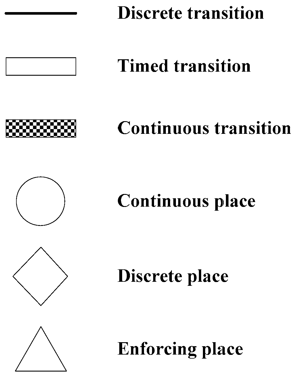
3. System Modeling with Petri Nets

With an OD being viewed as a control command, this work develops a method to schedule the system from a control perspective as done in [21,22]. Although the PN models in [31,32,33] are hybrid ones with both discrete and continuous places, they are not developed to describe the continuous material flows as required by the ODs. Thus, we modify the hybrid Petri net model presented in [21,22], due to the fact that they can describe the continuous material flows well. We first present models for devices including tanks and pipeline, then integrate them to develop the model for the whole system. A reader is referred to [34,35] for the basic knowledge of PN.

The above scheduling problem involves discrete-event variables, such as the source and destination of an OD, and continuous variables, such as volumes of crude oil and flow rates. Hence, both discrete and continuous places, and discrete and continuous transitions are needed to model the system. In the proposed PN model, a discrete place with a discrete token in it is used to implement the control logic of the system. A token in a continuous place can be treated as both discrete and continuous ones. When treated as a discrete one, it is used to describe some attributes such as if there is oil in a tank, and if the oil in a tank is ready to be discharged. When it is treated as a continuous one, it is used to describe the volume of oil in a tank. Note that a token in a continuous place indicates that there is oil in the tank modeled by the place. Also, a tank can hold one type of oil at a time. Thus, in the model, a continuous place can hold at most one token. If a token is sent to a continuous place that holds one token in it, the two tokens are merged into one with the volume being the sum. The flow rate of oil is described by the firing rate of a continuous transition. Moreover, colors are introduced to identify different types of crude oil, and time is also needed to describe the scheduling problem.

The proposed PN model is a kind of continuous-colored-timed PN (CCTPN) defined as CCTPN = (P_D∪P_C∪P_E, T_D∪T_T∪T_C, I, O, Ф, M₀), where P_D, P_C, and P_E are sets of discrete, continuous, and enforcing places, respectively; T_D, T_T, and T_C are sets of discrete, timed, and continuous transitions, respectively; I and O are input and output functions, respectively; Ф represents the color sets defined on tokens in places; and M₀ is the initial marking. The icons for the model are shown in Figure 1.

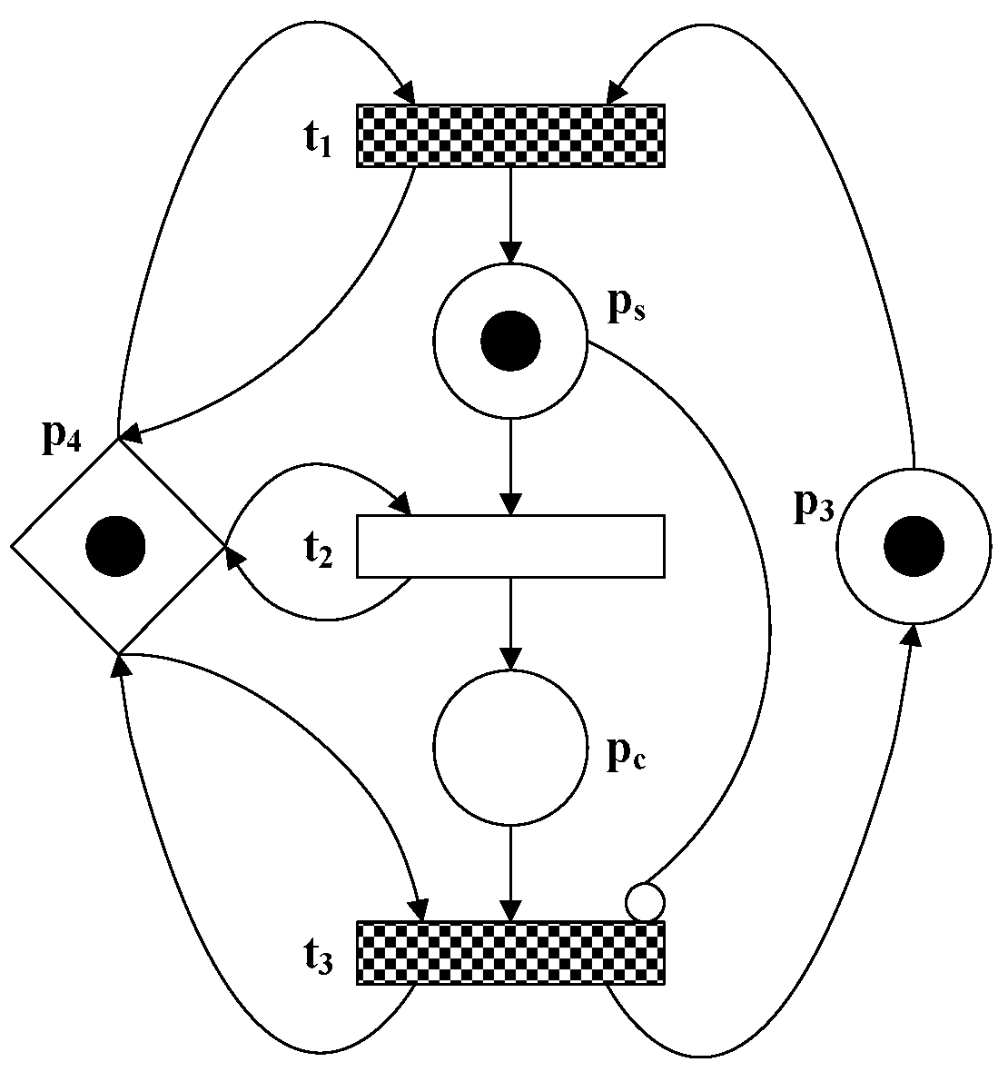
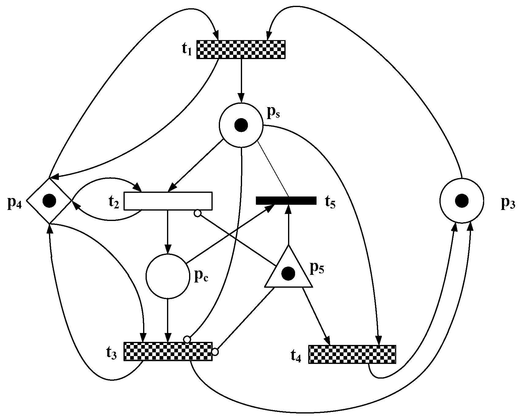
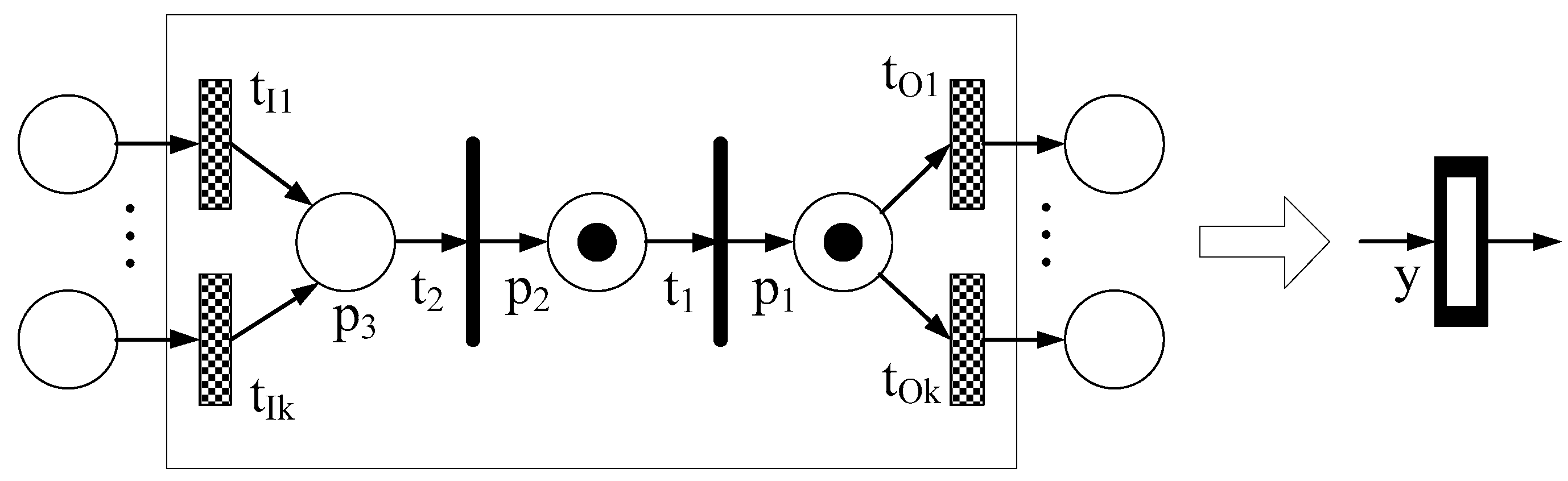
3.1. Device Modeling

The devices involved in crude oil operations include tanks (storage and charging tanks) and a pipeline. While scheduling a refinery without sufficient charging tanks, the crude oil must stay in storage tanks for ORT, but charging tanks may adopt the SCF mode during the execution of a schedule. Hence, the models for charging and storage tanks are different.

The PN model in Figure 2 describes the behavior of a storage tank and is the same as that in [21,22]. A storage tank is modeled by two continuous places p_s and p_c to describe its state. In the PN model, a token in a discrete place is treated as a discrete one and acts just as that in a general PN. For example, a token in p₄ is just a discrete one. A token in a continuous place can be treated as both discrete and continuous one. When it is treated as a discrete one, it indicates that there is oil in a tank. For example, one token in p_s or p_c or both denotes that there is oil in it. Also, when t₂ fires, the token in p_s is removed just like a discrete one. When the token in a continuous place is treated as a continuous one, it represents the crude oil in the device with a real number volume, which is called the token volume. If there is a token in an enforcing place, it enforces the output transitions to fire until it is empty.

A discrete transition behaves the same as in a general PN. When a timed transition fires, it moves a token from an input place to an output place with a constant time delay, which is used to model the oil residency time constraint. When a continuous transition fires, oil is delivered from one place to another with a flow rate for a time duration, which is determined by an OD. Hence, crude oil unloading, transportation or feeding to distillers can be modeled by continuous transitions.

One token in p_s indicates that the oil stays in the tank for less than ORT and is not ready for discharging. Only if there is a token in p_c, and p_s is empty, can the oil in the tank be discharged. Continuous place p₃ models the capacity of the tank available at the current marking. Continuous transitions t₁ and t₃ model the processing of charging to and discharging from a tank. Timed transition t₂ models the ORT constraint. When t₂ completes its firing with a given time delay, the token in p_s moves to p_c, indicating that the oil in the tank is ready for discharging. Notice that a non-emptied tank can be charged when the type of oil to be charged to the tank is same as that in the tank. In this case, when the firing of t₁ ends, both p_s and p_c hold a token such that both t₂ and t₃ are enabled. However, in this case, the firing of t₃ results in the violation of oil residency time constraint. Hence, inhibitor arc (p_s, t₃) guarantees that t₃ can fire only when p_s is emptied, which implies that the oil stays in the tank for ORT. If transition t₁ (t₂, t₃) fires, one token in place p₄ is consumed at the beginning, and one token is put into place p₄ when its firing ends. Since there is only one token in p₄, during the firing of one of transitions t₁, t₂, and t₃, the others are disabled, which ensures that a storage tank cannot be filled and discharged simultaneously. Thus, a storage tank can only be operated under the normal mode and its behavior is well described.

A charging tank should operate under the normal mode if possible. However, when the charging tanks in the system are not enough, the SCF mode has to be adopted to keep the distillers in operation. Thus, a charging tank should be modeled such that the behavior of both modes is described; the obtained PN model is shown in Figure 3. In this model, p_s, p_c, t₁, t₂, and t₃ are the same as for the storage tank shown in Figure 2. Transitions t₄ and t₅, and place p₅ are added to model the behavior of the SCF mode. Enforcing place p₅ that can hold at most one token at a time is a control place that decides the operation mode of a tank. If a charging tank starts to adopt the SCF mode, one token is created and put into p₅ such that t₂ and t₃ are disabled, and t₅ is forced to fire to move the token in p_c back to p_s immediately if p_c is not empty. At the same time, t₄ is forced to fire for feeding a distiller and t₁ can fire to charge the tank, i.e., the SCF mode is applied. When an instruction is received to end the SCF mode and switch to the normal mode, the token in p₅ is removed away. Then, t₄ is not enabled and cannot fire, and the tank goes back to the normal mode. Note that a charging tank can start to operate under the SCF mode, but the crude oil in it is no less than the safety stock, i.e., one token can be put into p₅ only if the sum of the volume associated with the token in p_s and p_c is greater than or equal to the safety stock. This can be decided by a schedule. In this way, the behavior of a charging tank is well modeled.

The PN model for a pipeline that can hold three different segments of crude oil is shown in Figure 4 and is the same as that in [21,22]. Places p₁–p₃ represent different oil segments in the pipeline. When discrete transitions t₁ and t₂ are enabled and fire, one token is moved from an input place into an output place immediately. Let T_I = {t_I1, …, t_Ik} and T_O = {t_O1, …, t_Ok}. As crude oil mixing is not considered here, the pipeline receives crude oil from only one storage tank and feeds only one charging tank with the same rate at a time. Hence, only one transition in T_I and one in T_O can fire with the same rate at a time. To simplify the PN model for the entire system, the pipeline is modeled in a hierarchical way and a macro transition y is used to describe the behavior of the pipeline when there is no confusion. In other words, when y fires, it implies that one transition in T_I and one in T_O fires at the same rate at the same time, which models the crude oil’s transport from storage tank to charging tank via a pipeline.

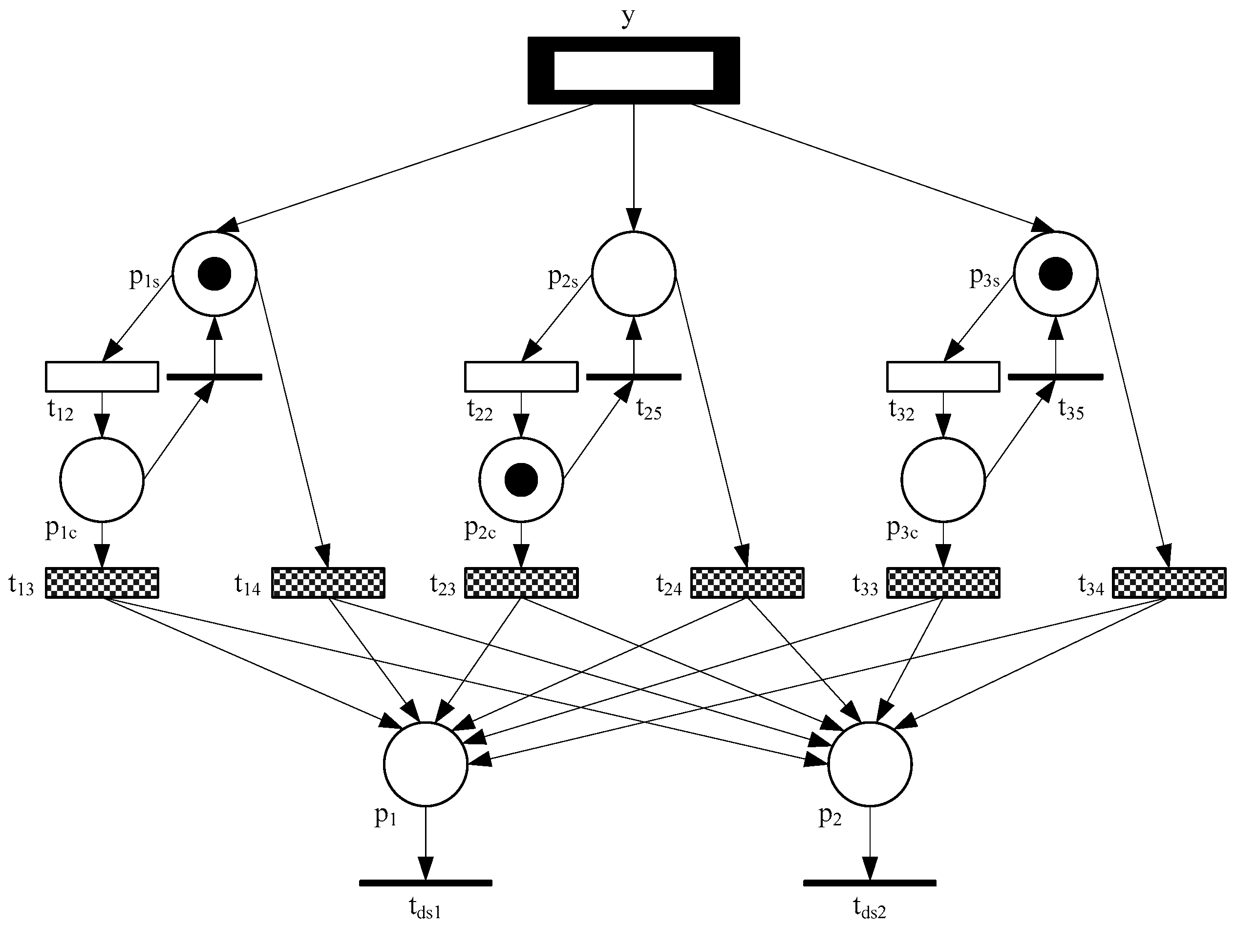
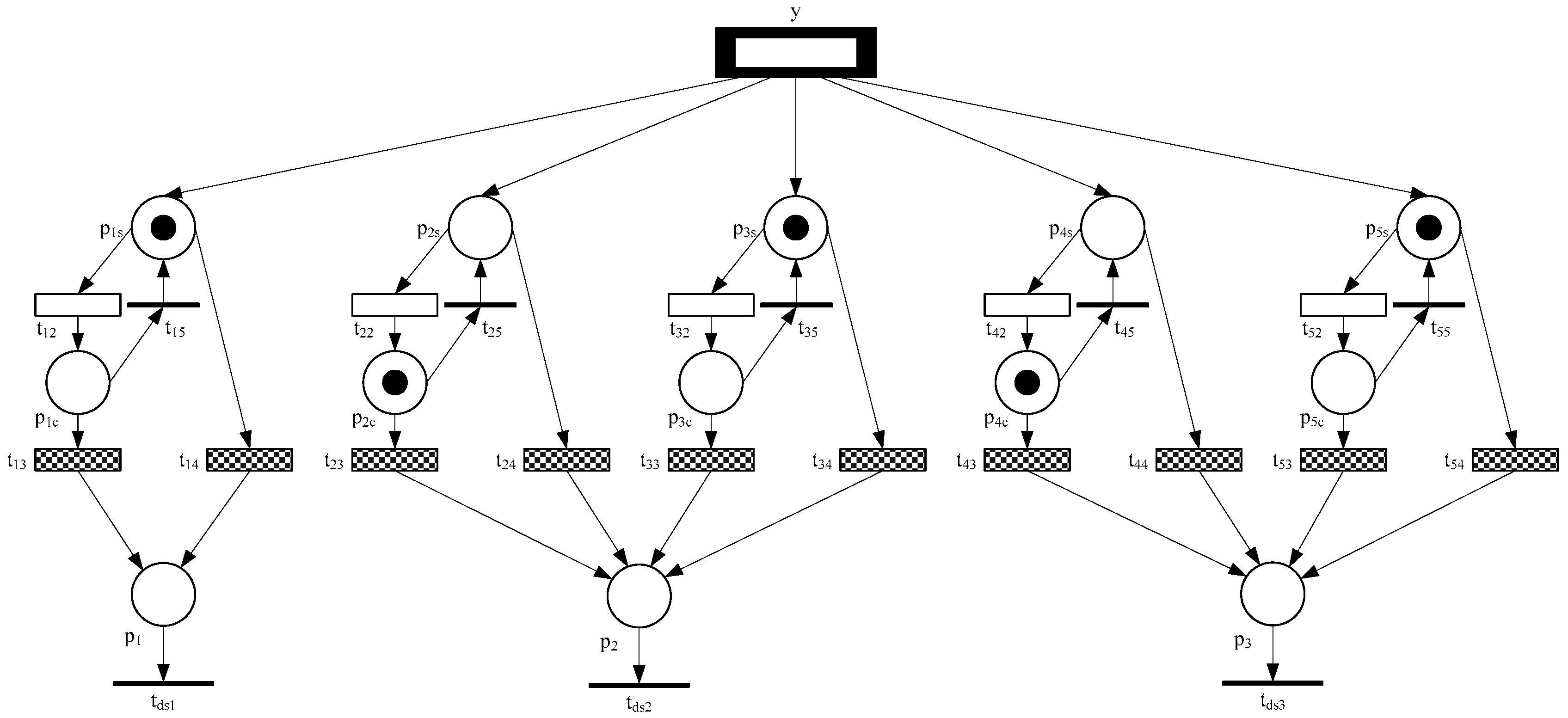
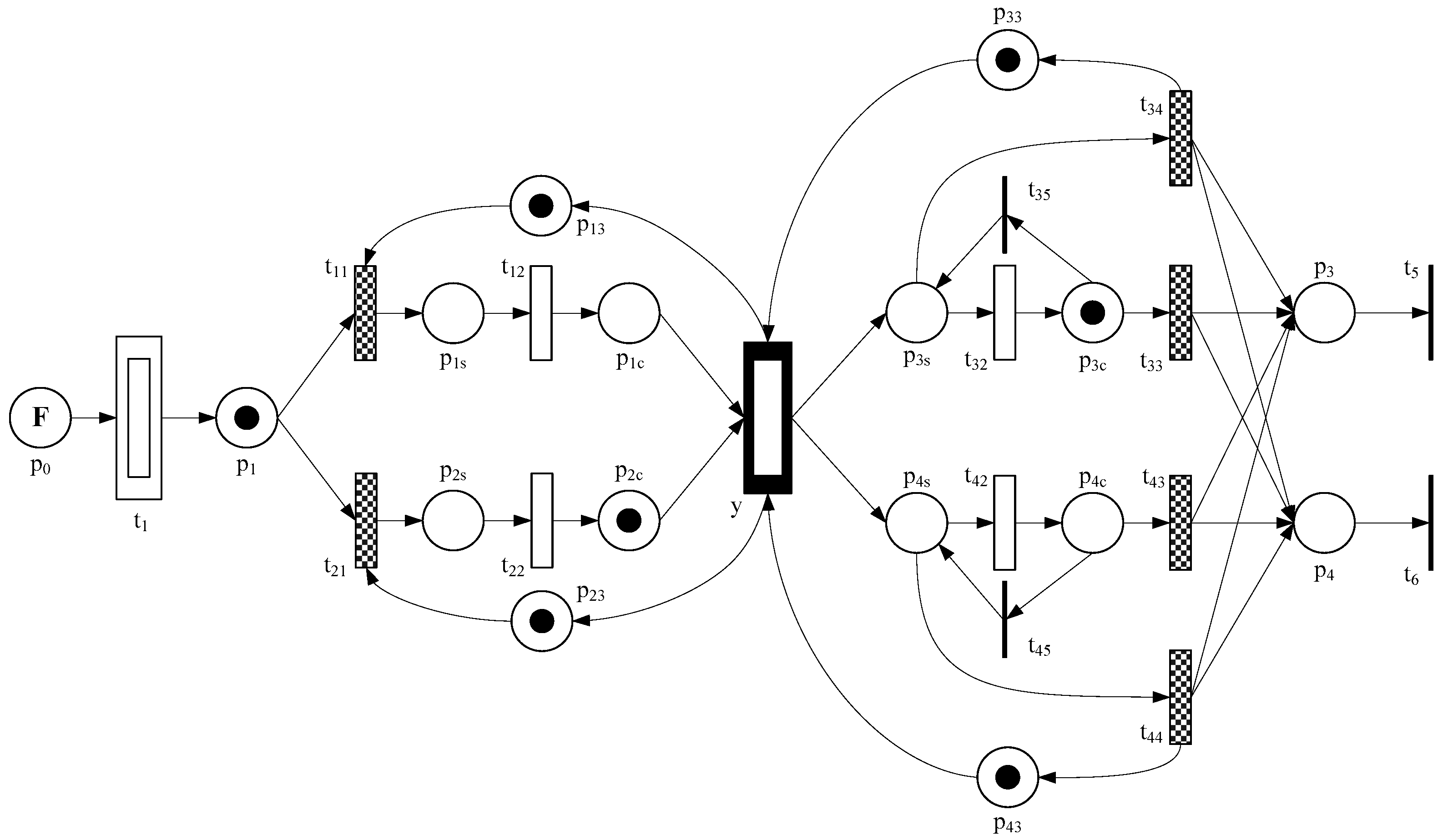
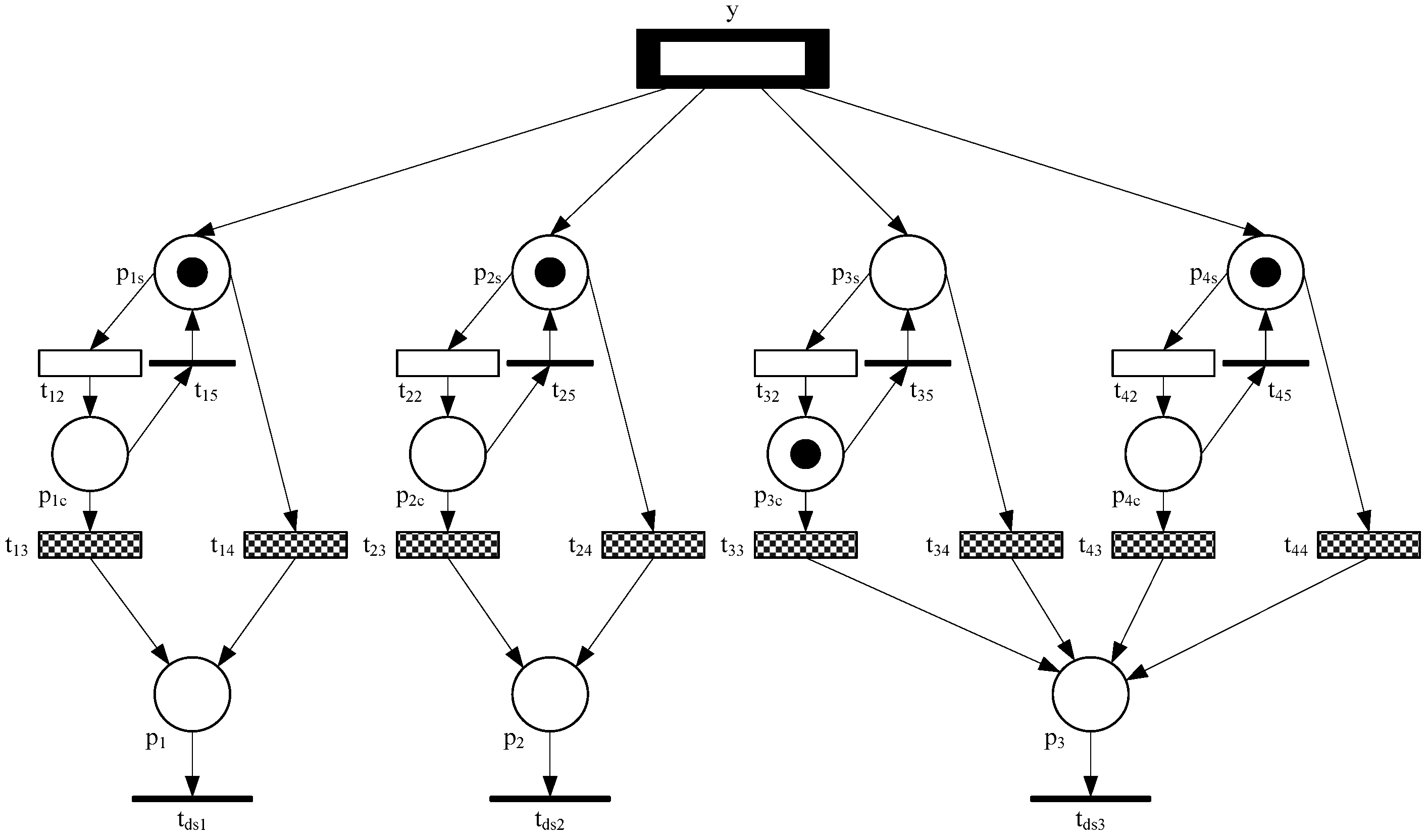
3.2. PN Model for the Whole System

The PN in Figure 5 models the whole system with two storage tanks, two charging tanks, and two distillers, where the discrete places, enforcing places, and their associated arcs, and the inhibitor arcs are omitted for concision. Crude oil is transported from storage tanks to charging tanks through a pipeline. Thus, y models both the discharging of storage tanks and the charging of charging tanks at the same time. In the model, {t₁₁, t₁₂, y, p_1s, p_1c, p₁₃} and {t₂₁, t₂₂, y, p_2s, p_2c, p₂₃} model the two storage tanks, while {y, t₃₂, t₃₃, t₃₄, t₃₅, p_3s, p_3c, p₃₃} and {y, t₄₂, t₄₃, t₄₄, t₄₅, p_4s, p_4c, p₄₃} model the two charging tanks.

Place p₀ with F tokens in it models a tanker carrying F types of crude oil when it arrives. Transition t₁ can fire to move one token from p₀ to p₁ only if p₁ is empty, and models that only one type of oil can be unloaded at a time. At the right part, places p₃ and p₄ model two distillers, and t₅ and t₆ represent distillation. However, it should be noted that the PN model just describes the structure of the system, not the detailed dynamics of the crude oil flow. From the definition of a short-term schedule, the firing of a continuous transition is triggered by an OD. Thus, with the flow rate given by ODs and the transition enabling and firing rules, the dynamics of the crude oil flow in the PN model can be defined.

The set of input places of transition t (input transitions of place p) is denoted as ^●t (^●p). Similarly, the set of output places of t (output transitions of p) is denoted as t^● (p^●). Furthermore, colors are introduced into the PN model to distinguish different types of crude oil and we let φ_i $\in$ Ф denote the crude oil type i, i.e., the color of a token in a place. At marking M, the number of tokens with color φ_i in p is denoted as M(p, φ_i) and the associated volume is denoted as V(M(p, φ_i)). It should be pointed out that V(M(p, φ_i)) = 0 implies M(p, φ_i) = 0. With the above symbols, readers are referred to [21,22] for the transition enabling and firing rules. Then, we can discuss the scheduling problem by using the developed model.

4. Scheduling Method

To obtain a feasible short-term schedule, the most difficult step is to decide on ODTs and ODFs. In this paper, we assume that a refining schedule is given, as can be found in the methods in [28,30]. Given a refining schedule that is set according to the crude oil availability during the scheduling horizon, the feeding rate to the distillers is known, which implies that there is enough crude oil in the storage tanks to be processed. Hence, finding a detailed schedule to realize a given refining schedule is independent of the number of storage tanks and their capacity, and the storage tanks in the system are ignored when a PN model is presented in the discussion thereafter.

According to Wu et al. [21,22], the existence of a feasible short-term schedule is the key to finding a schedule under the normal mode. With the SCF mode, a schedule should be available. Nevertheless, since the SCF mode is undesirable, its use should be minimized and the normal mode should be applied if possible. Thus, to schedule the system, we adopt both modes and the SCF mode is adopted only for some charging tanks during some periods when necessary. Under the normal mode, the system with initial state M₀ is said to be schedulable if there exists a feasible short-term schedule for a horizon (0, ∞) [21,22]. A state M is said to be safe if, with M as its initial state, the system is schedulable. Based on this safety concept, we discuss the scheduling problem to minimize the use of the SCF mode.

To minimize the use of the SCF mode, we need to measure such usage. When the SCF is applied for a charging tank by starting at time τ₁, this mode is applied without interruption until time τ₂. Then we say that, during time slot from τ₁ to τ₂, the SCF is applied to the charging tank. For a system with H charging tanks and K distillers, assume that charging tank CTK_i adopts the SCF mode for N_i time slots during the scheduling horizon. Let τ_sin and τ_ein denote the start and end time of the nth slot of applying the SCF mode for charging tank CTK_i, respectively. Then the total time during which the charging tanks adopt the SCF mode is defined as Π = ${\displaystyle {\sum }_{i=1}^H{\displaystyle {\sum }_{n=1}^{N_i}({\tau }_{ein}-{\tau }_{sin})}}$. Furthermore, let Γ = (τ_s, τ_e) be the scheduling horizon. Then the usage of the SCF mode can be measured by δ = Π/K(τ_e − τ_s), which gives the ratio of time during which the distillers are fed under the SCF mode. Hence, to minimize the usage of the SCF, we have to minimize δ. As the charging tanks are an important and limited resource, a utilization ratio is introduced to the charging tanks. A charging tank is at a working state if it is being charged, discharged, or t₂ in Figure 2 fires; otherwise it is at an idle state. Let N_i denote the number of time slots during which charging tank CTK_i is at a working state during the scheduling horizon, and ς_sin and ς_ein denote the start and end time of the nth working slot of CTK_i, respectively. Then, the utilization ratio of CTK_i is defined as ρ_i = ${\displaystyle {\sum }_{n=1}^{N_i}({\varsigma }_{ein}-{\varsigma }_{sin})}/({\tau }_e-{\tau }_s)$, and the utilization ratio for the whole system is defined as ρ = ${\displaystyle {\sum }_{i=1}^H{\rho }_i}/H$. We develop scheduling methods to find a schedule to minimize δ and increase ρ.

We use f_dsi, f_pmax, Ψ, and σ to denote the feeding rate to distiller DS_i, the maximal oil transportation rate of the pipeline, the ORT, and the safety stock, respectively. Places p_is and p_ic are used for charging tank CTK_i in the PN model. As a scheduling method, it is meaningful only if the production rate of the system can reach the maximum since productivity is a very important criterion. Hence, in the following discussion, for a refinery with K distillers, we assume that the system operates at the maximal production rate, or ${\displaystyle {\sum }_{k=1}^K{f}_{dsk}}$ = f_pmax, where f_dsk is the feeding rate to distiller DS_k.

For a refinery with only one distiller at the maximal production rate, as proven in [21], three charging tanks are necessary to schedule the operation under the normal mode, which can usually be satisfied in practice. Hence, we focus on analyzing a system with multiple distillers. For a system with K distillers, all the distillers have to process crude oil concurrently and uninterruptedly. Hence, at least one charging tank must be dedicated to a distiller, which implies that no schedule can be found even if the SCF mode is adopted if the number of charging tanks is less than K. Based on practical scenarios without sufficient charging tanks, for a refinery with K distillers and N charging tanks, we discuss the scheduling problem for cases with K ≤ N < 2K. Also, in the following discussion, we assume that each distiller processes different oil types since the obtained results in this case are applicable to cases when some distillers process the same oil type.

4.1. Systems with Two Distillers

In [21], it is shown that, under the normal mode, no feasible schedule with maximal production rate can be found for a refinery with one distiller and two charging tanks. Thus, it is clear that if there are only two charging tanks for a two-distiller system, to obtain a schedule, the two distillers must be fed by applying the SCF mode all the time, i.e., δ = 1. Then, we discuss the case with three charging tanks. For this case, with the PN model shown in Figure 6, we have the following results.

Proposition 1.

Assume that: (1) there are two distillers DS_1–2 with feeding rates f_ds1 and f_ds2, respectively, and α = Ψ × f_pmax, α₁ = Ψ × f_ds1, and α₂ = Ψ × f_ds2; (2) there are three charging tanks CTK_1–3 with capacities ξ₁, ξ₂, and ξ₃, respectively; (3) f_pmax = f_ds1 + f_ds2; and (4) initially, the volume of oil type 1 in CTK₁ is ζ₁, and the volumes of oil type 2 in CTK₂ and CTK₃ are ζ₂ and ζ₃, respectively. Then, a schedule can be found such that δ = 0.5 if Condition (3) holds:

$$\{\begin{array}{l}\sigma \le {\zeta }_1\le {\xi }_1-\mu \times {\alpha }_2\times f_{ds1}/f_{p\max }\\ {\zeta }_2={\alpha }_2\\ {\zeta }_3=\mu \times {\alpha }_2\end{array},$$

(3)

where μ Є [f_pmax/f_ds1, min{ξ₂/α₂, ξ₃/α₂}].

Proof. 

See Appendix A.1.

By the proof of the proposition, a method is given to find a schedule. To schedule the system, Condition (3) presents the necessary amount of oil that is initially in the charging tanks, which is easy to meet. In fact, if all the charging tanks are initially empty, no schedule can be found according to the operational requirements, no matter how many charging tanks there are. If there is more oil at the initial state, a schedule can be obtained similarly. By the obtained schedule, in order to keep DS₁ in operation, CTK₁ has to apply the SCF mode during the whole scheduling horizon due to the limited charging tanks. For DS₂, by carefully scheduling the system, it is alternately fed by two charging tanks, CTK₂ and CTK₃, under the normal mode. If one of them is empty, the other can be used to feed the distiller. Hence, both CTK₂ and CTK₃ operate under the normal mode during the whole scheduling horizon. To do so, the key is that every time CTK₁ (CTK₂, CTK₃) is charged, its volume is V₁ = μ × α₁ (V₂ = μ × α₂, V₂ = μ × α₂). Thus, a schedule can be found simply by using the proposed method.

Note that CTK₂ is empty during [τ₁, τ₂], and the utilization ratio of CTK₂ is ρ₂ = 1 – (μ × f_ds1 − f_pmax)/(μ × f_pmax) = 1 − f_ds1/f_pmax + 1/μ. Hence, CTK₂ is not fully utilized. If time duration [τ₁, τ₂] can be made longer than Ψ, CTK₂ can be used to feed DS₁ for some time under the normal mode such that δ can be reduced by the full use of CTK₂. Let ϖ = (μ × f_ds1 − 2 × f_pmax)/(f_ds1 + f_pmax). We have the following result.

Proposition 2.

Assume that: (1) there are two distillers DS_1‒2 with feeding rates f_ds1 and f_ds2, respectively, and α = Ψ × f_pmax, α₁ = Ψ × f_ds1, and α₂ = Ψ × f_ds2; (2) there are three charging tanks CTK_1–3 with capacities ξ₁, ξ₂, and ξ₃, respectively; (3) f_pmax = f_ds1 + f_ds2; and (4) initially, the volume of oil type 1 in CTK₁ is ζ₁, and the volumes of oil type 2 in CTK₂ and CTK₃ are ζ₂ and ζ₃, respectively. Then, a schedule can be obtained such that δ = (μ − ϖ)/2μ if Condition (4) holds:

$$\{\begin{array}{l}\sigma \le {\zeta }_1\le {\xi }_1-{\alpha }_2\\ \sigma -{\alpha }_2+\varpi \times {\alpha }_1\times f_{ds1}/f_{p\max }\le {\zeta }_1\le {\xi }_1-\mu \times {\alpha }_2\times f_{ds1}/f_{p\max }\\ {\zeta }_2={\alpha }_2\\ {\zeta }_3=\mu \times {\alpha }_2\end{array},$$

(4)

where μ Є [max{(ϖ × f_ds1 + f_pmax)/f_ds1, 2f_pmax/f_ds1}, min{ξ₂/α₂, ξ₃/α₂}] and ϖ Є [0, min{ξ₂/α₁, ξ₃/α₁}].

Proof. 

See Appendix A.2.

This schedule is obtained by modifying that created by Proposition 1. By the scheduling method given in the proof of Proposition 2, DS₂ is fed by CTK₂ and CTK₃ under the normal mode during the whole scheduling horizon, which is the same as that in Proposition 1. However, since CTK₂ and CTK₃ have idle time for feeding DS₂, they can feed DS₁ under the normal mode during their idle time such that the usage of the SCF mode is reduced. To do so, when the charging tanks are charged with volume V₁ = μ × α₁ of oil type 1, we do not charge all the crude oil into CTK₁ at one time as done in Proposition 1; instead, V₁ is divided into three parcels and charged in the following order: charge CTK₁ with volume v₁ = α₁ → charge CTK₂ or CTK₃ with volume v₂ = ϖ × α₁ → charge CTK₁ with volume v₃ = (μ − ϖ − 1)α₁. By doing so, when the crude oil of type 1 in CTK₂ or CTK₃ is ready for discharging under the normal mode, it can be used to feed DS₁ until it is used up. Note that, by doing so, DS₂ is still fed under the normal mode.

For the obtained schedule using Proposition 2, CTK₂ is used to feed DS₂ and DS₁ during [τ₀, τ₁] and [τ₃, τ₄] under the normal mode, respectively. In this way, the utilization ratio of CTK₂ reaches ρ₂ = 1. Furthermore, CTK₁ and CTK₃ are occupied during the whole scheduling horizon too. Hence, δ is minimized and cannot be reduced any more. It should be pointed out that such a schedule can be obtained only if μ ≥ max{(ϖ × f_ds1 + f_pmax)/f_ds1, 2f_pmax/f_ds1}, otherwise, CTK₂ cannot be used to feed DS₁ under the normal mode, and the system has to be scheduled using Proposition 1.

4.2. Scheduling a System with Three Distillers

For a system with three distillers, the scheduling problem is much more complicated than with two distillers. For such a system, if there are three charging tanks, it is obvious that we can use one tank to feed one distiller under the SCF mode and δ = 1. We then discuss cases with more than three charging tanks.

4.2.1. Case 1: Four Charging Tanks

The PN model for the system with three distillers and four charging tanks is shown in Figure 7. In this case, only one charging tank can be assigned to each of DS₁ and DS₂, and two charging tanks are assigned to DS₃. Then, we present methods to schedule the system.

Proposition 3.

Assume that: (1) there are three distillers DS_1–3 with feeding rates f_ds1, f_ds2, and f_ds3, respectively, and α = Ψ × f_pmax, α₁ = Ψ × f_ds1, α₂ = Ψ × f_ds2, and α₃ = Ψ × f_ds3; (2) there are four charging tanks CTK_1–4 with capacities ξ₁, ξ₂, ξ₃, and ξ₄, respectively; (3) f_pmax = f_ds1 + f_ds2 + f_ds3; and (4) initially, the volume of oil type 1 (2; 3; 3) in CTK₁ (CTK₂; CTK₃; CTK₄) is ζ₁ (ζ₂; ζ₃; ζ₄). Then, if Condition (5) holds, we can find a schedule with δ = 2/3.

$$\{\begin{array}{l}\sigma \le {\zeta }_1\le {\xi }_1-\mu \times \left(\alpha -{\alpha }_1\right)\times f_{ds1}/f_{p\max }\\ \sigma +\mu \times {\alpha }_1\times f_{ds2}/f_{p\max }\le {\zeta }_2\le {\xi }_2-\mu \times \left(\alpha -{\alpha }_1-{\alpha }_2\right)\times f_{ds2}/f_{p\max }\\ {\zeta }_3={\alpha }_3\\ {\zeta }_4=\mu \times {\alpha }_3\end{array},$$

(5)

where μ Є [f_pmax/(f_ds1 + f_ds2), min{ξ₃/α₃, ξ₄/α₃}].

Proof. 

See Appendix A.3.

Similar to Proposition 1, if two charging tanks are assigned to a distiller, this distiller can be fed under the normal mode during the whole scheduling horizon. For the distiller with only one charging tank being assigned, the SCF mode has to be applied. Just as in Proposition 1, the key to the proposed method is that every time crude oil of type 1 (2, 3) is charged, the volume of oil to be charged is V₁ = μ × α₁ (V₂ = μ × α₂, V₃ = μ × α₃).

With the obtained schedule by using the method given by Proposition 3, charging tank CTK₃ is emptied at time τ₀ + Ψ and it is kept to be empty until it starts to be charged at time τ₁. Hence, CTK₃ is not fully utilized and its utilization ratio is ρ₃ = 1 − (μ × f_ds1 + μ × f_ds2 − f_pmax)/(μ × f_pmax) = 1 − (f_ds1 + f_ds2)/f_pmax + 1/μ. Similar to the situation in Proposition 1, CTK₃ can be used to reduce the usage of the SCF mode. Let ϖ = (μ × f_ds1 + μ × f_ds2 − 2 × f_pmax)/(f_ds2 + f_pmax). We have the following result.

Proposition 4.

Assume that: (1) there are three distillers DS_1–3 with feeding rates f_ds1, f_ds2, and f_ds3, respectively, and α = Ψ × f_pmax, α₁ = Ψ × f_ds1, α₂ = Ψ × f_ds2, α₃ = Ψ × f_ds3, and f_ds1 ≥ f_ds2; (2) there are four charging tanks CTK_1–4 with capacities ξ₁, ξ₂, ξ₃, and ξ₄, respectively; (3) f_pmax = f_ds1 + f_ds2 + f_ds3; and (4) initially, the volume of oil type 1 (2; 3; 3) in CTK₁ (CTK₂; CTK₃; CTK₄) is ζ₁ (ζ₂; ζ₃; ζ₄). Then, if Condition (6) holds, we can find a schedule with δ = (2μ − ϖ)/3μ.

$$\{\begin{array}{l}\sigma \le {\zeta }_1\le {\xi }_1-{\alpha }_2-{\alpha }_3\\ \sigma -{\alpha }_2-{\alpha }_3+\varpi \times {\alpha }_2\times f_{ds1}/f_{p\max }\le {\zeta }_1\le {\xi }_1-\left(\mu \times \alpha -\varpi \times {\alpha }_2-\mu \times {\alpha }_1\right)\times f_{ds1}/f_{p\max }\\ \sigma +\left(\mu \times {\alpha }_1+\varpi \times {\alpha }_2\right)\times f_{ds2}/f_{p\max }\le {\zeta }_2\le {\xi }_2-\left(\mu \times \alpha -\varpi \times \alpha -\mu \times {\alpha }_1-\mu \times {\alpha }_2\right)\times f_{ds2}/f_{p\max }\\ {\zeta }_3={\alpha }_3\\ {\zeta }_4=\mu \times {\alpha }_3\end{array},$$

(6)

where μ Є [max{(ϖ×f_ds2 + f_pmax)/(f_ds1 + f_ds2), 2f_pmax/(f_ds1 + f_ds2)}, min{ξ₃/α₃, ξ₄/α₃}] and ϖ Є [0, min{ξ₃/α₂, ξ₄/α₂}].

Proof. 

See Appendix A.4.

For this proposed scheduling method, CTK₃ or CTK₄ is used to feed DS₂ under the normal mode for some time. Similar to Proposition 2, when CTK₃ or CTK₄ finishes feeding DS₃ and becomes empty, it is charged with volume v = ϖ × α₂ of oil type 2. When the crude oil in it is ready for feeding under the normal mode, it starts feeding DS₂ until it is empty, resulting in the reduction of the SCF mode operation time of CTK₂.

By the above obtained schedule, all the charging tanks including CTK₃, which has idle time for the schedule obtained by using Proposition 3, are fully utilized and the utilization ratio for the system is ρ = 1. Thus, δ cannot be reduced further and the schedule is optimal in terms of the minimization of δ. Notice that, if CTK₃ is charged with oil type 1 instead of oil type 2 with volume ϖ’ × α₁ when it is emptied at τ₁, where ϖ’ = (μ × f_ds1 + μ × f_ds2 − 2 × f_pmax)/(f_ds1 + f_pmax), the system can be scheduled similarly. Consequently, we have Π’ = (2μ – ϖ’) × Ψ ≤ (2μ − ϖ) × Ψ = Π as f_ds1 ≥ f_ds2. Hence, charging oil of type 2 into CTK₃ is better than charging oil of type 1 into it at time τ₁.

4.2.2. Case 2: Five Charging Tanks

Now we discuss the situation where there are five charging tanks and three distillers, and the PN model for it is shown in Figure 8. For this system, DS₁ has only one charging tank, and the other two distillers have two charging tanks each.

Proposition 5.

Assume that: (1) there are three distillers DS_1‒3 with feeding rates f_ds1, f_ds2, and f_ds3, respectively, and α = Ψ × f_pmax, α₁ = Ψ × f_ds1, α₂ = Ψ × f_ds2, and α₃ = Ψ × f_ds3; (2) there are five charging tanks CTK_1–5 with capacities ξ_1–5, respectively; (3) f_pmax = f_ds1 + f_ds2 + f_ds3; and (4) initially, the volume of oil type 1 (2; 2; 3; 3) in CTK₁ (CTK₂; CTK₃; CTK₄; CTK₅) is ζ₁ (ζ₂; ζ₃; ζ₄; ζ₅). Then, if Condition (7) holds, a schedule can be found with δ = 1/3.

$$\{\begin{array}{l}\sigma \le {\zeta }_1\le {\xi }_1-\mu \times \left(\alpha -{\alpha }_1\right)\times f_{ds1}/f_{p\max }\\ {\zeta }_2={\alpha }_2\\ {\zeta }_3=\mu \times {\alpha }_2\\ {\zeta }_4={\alpha }_3\\ {\zeta }_5=\mu \times {\alpha }_3\end{array},$$

(7)

where μ Є [f_pmax/f_ds1, min {ξ₂/α₂, ξ₃/α₂, ξ₄/α₃, ξ₅/α₃}].

Proof. 

See Appendix A.5.

By the obtained schedule for this case, the system is operated similarly to Propositions 1 and 3. CTK₂ and CTK₄ are empty and idle during [τ₁, τ₂] and [τ₁, τ₂ + (μ × α₂)/f_pmax], respectively, and their utilization ratios for these two charging tanks are ρ₂ = 1 − (μ × f_ds1 − f_pmax)/(μ × f_pmax) and ρ₄ = 1 − (μ × f_ds1 + μ × f_ds2 − f_pmax)/(μ × f_pmax), respectively. Thus, it is possible to use CTK₂ and/or CTK₄ to feed DS₁ under the normal mode so as to reduce δ. By following this idea, we schedule the system as follows. Let ϖ = (μ × f_ds1 + μ × f_ds2 − 2 × f_pmax)/(f_ds1 + f_pmax). We have the following result.

Proposition 6.

Assume that: (1) there are three distillers DS_1–3 with feeding rates f_ds1, f_ds2, and f_ds3, respectively, and α = Ψ × f_pmax, α₁ = Ψ × f_ds1, α₂ = Ψ × f_ds2, α₃ = Ψ × f_ds3, and f_ds2 ≥ f_ds3; (2) there are five charging tanks CTK_1–5 with capacities ξ_1–5, respectively; (3) f_pmax = f_ds1 + f_ds2 + f_ds3; and (4) initially, the volume of oil type 1 (2; 2; 3; 3) in CTK₁ (CTK₂; CTK₃; CTK₄; CTK₅) is ζ₁ (ζ₂; ζ₃; ζ₄; ζ₅). Then, if Condition (8) holds, a schedule can be found with δ = (μ − ϖ)/3μ.

$$\{\begin{array}{l}\sigma \le {\zeta }_1\le {\xi }_1-{\alpha }_2-{\alpha }_3\\ \sigma -{\alpha }_2-{\alpha }_3+\varpi \times {\alpha }_1\times f_{ds1}/f_{p\max }\le {\zeta }_1\le {\xi }_1-\left(\mu \times \alpha -\varpi \times \alpha -\mu \times {\alpha }_1\right)\times f_{ds1}/f_{p\max }\\ {\zeta }_2={\alpha }_2\\ {\zeta }_3=\mu \times {\alpha }_2\\ {\zeta }_4={\alpha }_3\\ {\zeta }_5=\mu \times {\alpha }_3\end{array},$$

(8)

where μ Є [max{(ϖ × f_ds1 + f_pmax)/f_ds1, 2f_pmax/(f_ds1 + f_ds2)}, min{ξ₂/α₂, ξ₃/α₂, ξ₄/α₃, ξ₅/α₃}] and ϖ Є [0, min{ξ₄/α₁, ξ₅/α₁}].

Proof. 

See Appendix A.6.

The schedule generated by Proposition 6 is based on that obtained by Proposition 5. The difference is that CTK₄ is used to feed DS₁ under the normal mode for some time due to that CTK₄ has idle time for the schedule obtained by Proposition 5. Thus, by using the scheduling method given in Proposition 6, CTK₄ is fully utilized, but CTK₂ is empty and idle during [τ₀ + Ψ, τ₀ + (μ × α₁)/f_pmax], i.e., the utilization ratio for CTK₂ and CTK₄ is ρ₂ = 1 − (μ × f_ds1 − f_pmax)/(μ × f_pmax) and ρ₄ = 1, respectively. In this case, we cannot make ρ = 1 for the entire system, since both CTK₂ and CTK₄ are emptied at time τ₀ + Ψ but only one of them can be charged at a time. Moreover, if we charge CTK₂ with oil type 3 instead of oil type 2 at time τ₀ + (μ × α₁)/f_pmax, the system can be scheduled similarly and the time taken for CTK₁ to feed DS₁ under the SCF mode is reduced to ϖ’ ×Ψ = (μ × f_ds1 + μ × f_ds3 − 2 × f_pmax)/(f_ds1 + f_pmax) × Ψ ≤ ϖ × Ψ as f_ds2 ≥ f_ds3 holds. Note that the charging of CTK₁ is completed at time τ₀ + (μ × α₁)/f_pmax and does not feed DS₁ during [τ₂ − ϖ × Ψ, τ₂]. If τ₂ − max{τ₀ + (μ × α₁)/f_pmax, τ₂ − ϖ × Ψ} ≥ Ψ holds, CTK₁ can feed DS₁ under the normal mode during [τ₂, τ₃], which implies δ = (μ − ϖ)/3μ − f_ds3/3f_pmax. Moreover, we can further reduce δ by increasing the utilization of both CTK₂ and CTK₄ rather than just one of them. By doing so, a more complex schedule with a large number of charging tank switches may be obtained. However, δ is reduced slightly such that the obtained schedule is not meaningful in practice. Nevertheless, it is applicable for a system with more than three distillers, which is discussed in the next section.

5. Scheduling for General Systems

In the last section, we discussed the scheduling problem for different cases. In this section, we extend these results to a general system with K distillers. For a system with K distillers and K charging tanks, it is obvious that a schedule with one tank feeding one distiller under the SCF mode can be found such that δ = 1. Then, we discuss the case with 2K − N charging tanks, where N < K.

Case 1: 2K − N Charging Tanks

For a system with K distillers and 2K − N charging tanks, where N < K, only one charging tank is assigned to each of distiller DS_1‒N, and the other distillers have two charging tanks. Let charging tank CTK_i be represented by {p_is, p_ic, t_i2, t_i3, t_i4, t_i5} and distiller DS_i be represented by p_i in a PN model. Then, we present the following results.

Proposition 7.

Assume that: (1) there are K ≥ 3 distillers DS_1‒K with feeding rates f_ds1–f_dsK, and α = Ψ × f_pmax, α₁ = Ψ × f_ds1, α₂ = Ψ × f_ds2, …, α_K = Ψ × f_dsK; (2) there are 2K − N (N < K) charging tanks CTK_{1–(2K − N)} with capacities ξ_1–(2K−N); (3) f_pmax = f_ds1 + f_ds2 + … + f_dsK; and (4) initially, the volume of oil type 1 (i; j; j) in CTK₁ (CTK_i; CTK_(2j−N−1); CTK_(2j−N)) is ζ₁ (ζ_i; ζ_(2j−N−1); ζ_(2j−N)), i Є {2, 3, …, N} and j Є {N + 1, N + 2, …, K}. Then, if Condition (9) holds, a schedule can be found with δ = N/K.

$$\{\begin{array}{l}\sigma \le {\zeta }_1\le {\xi }_1-\mu \times \left(\alpha -{\alpha }_1\right)\times f_{ds1}/f_{p\max }\\ \dots \\ \sigma +\mu \times {\displaystyle {\sum }_{k=1}^{i-1}{\alpha }_k}\times f_{dsi}/f_{p\max }\le {\zeta }_i\le {\xi }_i-\mu \times \left(\alpha -{\displaystyle {\sum }_{k=1}^i{\alpha }_k}\right)\times f_{dsi}/f_{p\max }\\ \dots \\ \sigma +\mu \times {\displaystyle {\sum }_{k=1}^{N-1}{\alpha }_k}\times f_{dsN}/f_{p\max }\le {\zeta }_N\le {\xi }_N-\mu \times \left(\alpha -{\displaystyle {\sum }_{k=1}^N{\alpha }_k}\right)\times f_{dsN}/f_{p\max }\\ {\zeta }_{\left(N+1\right)}={\alpha }_{\left(N+1\right)}\\ {\zeta }_{\left(N+2\right)}=\mu \times {\alpha }_{\left(N+1\right)}\\ \dots \\ {\zeta }_{\left(2j-N-1\right)}={\alpha }_j\\ {\zeta }_{\left(2j-N\right)}=\mu \times {\alpha }_j\\ \dots \\ {\zeta }_{\left(2K-N-1\right)}={\alpha }_K\\ {\zeta }_{\left(2K-N\right)}=\mu \times {\alpha }_K\end{array},$$

(9)

where μ Є [f_pmax/(f_ds1 + f_ds2 + … + f_dsN), min{ξ_(N+1)/α_(N+1), ξ_(N+2)/α_(N+1), …, ξ_(2j−N−1)/α_j, ξ_(2j−N)/α_j, …, ξ_(2K−N−1)/α_K, ξ_(2K−N)/α_K}].

Proof. 

See Appendix A.7.

Proposition 7 extends Propositions 1, 3, and 5 and presents a scheduling method for a general system with K distillers and 2K − N charging tanks. By the method given in Proposition 7, every time a charging tank for feeding distiller DS_i, i Є {1, 3, …, K}, is charged, μ × α_i of oil is charged no matter what the operation mode of the charging tank is. Also, if the normal mode is applied, a charging tank is emptied after feeding a distiller. Thus, a schedule is easily found.

Note that charging tanks CTK_2j−N are empty during [τ₀ + Ψ, τ₀ + μ × (α₁ + α₂ + … + α_j−1)/f_pmax], j Є {N + 1, N + 2, …, K}, and can be used to reduce δ. Hence, among these charging tanks, Q tanks with 1 ≤ Q ≤ min{N, K − N} can be used to feed DS_{(N−Q+1)−N} under the normal mode. Let ϖ₁ = (μ × f_ds1 + μ × f_ds2 + … + μ × f_ds(K−Q) − 2 × f_pmax)/(f_ds(N−Q+1) + f_pmax), and ϖ_q = (μ × f_ds1 + μ × f_ds2 + … + μ × f_{ds(q+K−Q−1)} – 2 × f_pmax − ϖ₁ × f_ds(N−Q+1) − ϖ₂ × f_ds(N−Q+2) − … − ϖ_(q−1) × f_{ds(q+N−Q−1)})/(f_ds(q+N−Q) + f_pmax), q Є {2, 3, …, Q}, ϖ = ϖ₁ + ϖ₂ + … + ϖ_Q and Ω_q = (ϖ₁ × α_(N−Q+1) + ϖ₂ × α_(N−Q+2) + … + ϖ_q × α_(q+N−Q))/f_pmax. Further, let ε_i = μ × α_i/f_pmax if 1 ≤ i ≤ N − Q + 1 and ε_i = (μ − ϖ_(i−N+Q))×α_i/f_pmax if N − Q + 1 < i ≤ N. Then, there exists an integer L such that ε₁ + ε₂ + … + ε_(L−1) ≤ Ψ ≤ ε₁ + ε₂ + … + ε_L and 1 ≤ L ≤ N hold. We present the following results.

Proposition 8.

Assume that: (1) there are K ≥ 3 distillers DS_1–K with feeding rates f_ds1‒f_dsK, and α = Ψ × f_pmax, α₁ = Ψ × f_ds1, α₂ = Ψ × f_ds2, …, α_K = Ψ × f_dsK, f_ds1 ≥ f_ds2 ≥ … ≥ f_dsN and f_{ds(N + 1)} ≥ f_{ds(N + 2)} ≥ … ≥ f_dsK; (2) there are 2K − N (N < K) charging tanks CTK_1–(2K−N) with capacities ξ_1‒(2K−N); (3) f_pmax = f_ds1 + f_ds2 + … + f_dsK; and (4) initially, the volume of oil type 1 (i; L; l; j; j) in CTK₁ (CTK_i; CTK_L; CTK_l; CTK_(2j−N−1); CTK_(2j−N)) is ζ₁ (ζ_i; ζ_L; ζ_l; ζ_(2j−N−1); ζ_(2j−N)), where i $\mathit{\in }$ {2, 3, …, L − 1}, l $\mathit{\in }$ { L + 1, L + 2, …, N}, and j Є {N + 1, N + 2, …, K}. Then, if Condition (10) holds, a schedule can be found with δ = (N × μ − ϖ)/(K × μ).

$$\{\begin{array}{l}\sigma \le {\zeta }_1\le {\xi }_1-{\epsilon }_1\times f_{p\max }+{\epsilon }_1\times f_{ds1}\\ \dots \\ \sigma +{\displaystyle {\sum }_{k=1}^{i-1}{\epsilon }_k}\times f_{dsi}\le {\zeta }_i\le {\xi }_i-{\epsilon }_i\times f_{p\max }+{\displaystyle {\sum }_{k=1}^i{\epsilon }_k}\times f_{dsi}\\ \dots \\ \sigma +{\displaystyle {\sum }_{k=1}^{L-1}{\epsilon }_k}\times f_{dsL}\le {\zeta }_L\le {\xi }_L-\alpha +{\displaystyle {\sum }_{k=1}^{L-1}{\epsilon }_k}\times f_{p\max }+{\alpha }_L\\ \sigma -\alpha +{\displaystyle {\sum }_{k=1}^{L-1}{\epsilon }_k}\times f_{p\max }+\mathsf{\Omega }\times f_{dsL}\le {\zeta }_L\le {\xi }_L-{\epsilon }_L\times f_{p\max }+{\displaystyle {\sum }_{k=1}^L{\epsilon }_k}\times f_{dsL}+{\mathsf{\Omega }}_L\times f_{dsL}\\ \dots \\ \sigma +{\displaystyle {\sum }_{k=1}^{l-1}{\epsilon }_k}\times f_{dsl}+\mathsf{\Omega }\times f_{dsl}\le {\zeta }_l\le {\xi }_l-{\epsilon }_l\times f_{p\max }+{\displaystyle {\sum }_{k=1}^l{\epsilon }_k}\times f_{dsl}+{\mathsf{\Omega }}_l\times f_{dsl}\\ \dots \\ \sigma +{\displaystyle {\sum }_{k=1}^{N-1}{\epsilon }_k}\times f_{dsN}+\mathsf{\Omega }\times f_{dsN}\le {\zeta }_N\le {\xi }_N-{\epsilon }_N\times f_{p\max }+{\displaystyle {\sum }_{k=1}^l{\epsilon }_N}\times f_{dsl}+{\mathsf{\Omega }}_N\times f_{dsN}\\ {\zeta }_{\left(N+1\right)}={\alpha }_{\left(N+1\right)}\\ {\zeta }_{\left(N+2\right)}=\mu \times {\alpha }_{\left(N+1\right)}\\ \dots \\ {\zeta }_{\left(2j-N-1\right)}={\alpha }_j\\ {\zeta }_{\left(2j-N\right)}=\mu \times {\alpha }_j\\ \dots \\ {\zeta }_{\left(2K-N-1\right)}={\alpha }_K\\ {\zeta }_{\left(2K-N\right)}=\mu \times {\alpha }_K\end{array}$$

(10)

where μ Є [max{(ϖ₁ × f_ds(N−Q+1) + ϖ₂ × f_ds(N−Q+2) + … + ϖ_Q × f_dsN + f_pmax)/(f_ds1 + f_ds2 + … + f_dsN), 2f_pmax/(f_ds1 + f_ds2 + … + f_ds(K−Q))}, min{ξ_(N+1)/α_(N+1), ξ_(N+2)/α_(N+1), …, ξ_(2j−N−1)/α_j, ξ_(2j−N)/α_j, …, ξ_(2K−N−1)/α_K, ξ_(2K–N)/α_K}], ϖ₁ Є [0, min{ξ_{(2K−2Q−N+1)}/α_(N−Q+1), ξ_{(2K−2Q−N+2)}/α_(N−Q+1)}], ϖ₂ Є [0, min{ξ_{(2K−2M−Q+3)}/α_(N−Q+2), ξ_{(2K−2M−Q+4)}/α_(N−Q+2)}], …, and ϖ_Q Є [0, min{ξ_(2K−N−1)/α_N, ξ_(2K−N)/α_N}].

Proof. 

See Appendix A.8.

Proposition 8 is the extension of Propositions 2, 4, and 6 and presents a method to find a schedule for a general situation with 2K − N charging tanks. The method given by Proposition 8 improves the one given by Proposition 7 by using the idle time of charging tanks to feed distillers under the normal mode. Thus, one needs to examine the idle time of such charging tanks and schedule the idle time by the method given in Proposition 8. The key is that, during the idle time of charging tank CTK_{(2q+2K−2Q N−1)} or CTK_{(2q+2K−2Q−N)}, q Є {1, 2, …, Q}, for feeding DS_(q+K−Q), it is charged with volume ϖ_q × α_(q+N–Q) of oil type (q + N − Q), and feed DS_(q+N−Q) under the normal mode for some time. However, the total volume of oil type k, k Є {1, 2, …, K} that is charged into charging tanks remains V_k = μ × α_k, which is the same as that in Proposition 7. However, for oil of type i, i Є {1, 2, …, N}, it may be divided into several parts and charged into the charging tanks sequentially according to the proposed method.

Note that, in order to reduce the number of switches in feeding distillers, we usually take the maximal value of μ. While adopting Proposition 8, the maximal μ is calculated first. Then, this value is used to calculate the corresponding ϖ. By examining the upper and lower bounds of μ and ϖ, we can decide Q and obtain the corresponding schedule. Note that the charging of CTK_q is completed at time τ_q = τ₀ + ε₁ + ε₂ + … + ε_q if q < L and τ_q = τ₀ + ε₁ + ε₂ + … + ε_q + Ω_Q if q ≥ L. If (τ₁ + Ω_q + (1 + ϖ_q) × Ψ) − max{τ_q, τ₁ + Ω_q + Ψ} ≥ Ψ holds, CTK_q can feed DS_q under the normal mode during [τ₁ + Ω_q + (1 + ϖ_q) × Ψ, τ₂], which further reduces δ.

In the proposed scheduling method, the initial crude oil in the charging tanks should meet the given requirement. For charging tanks CTK_1−N, the lower bound can be easily satisfied as σ is not large and there is usually crude oil in the charging tanks initially in practice. If the volume of initial crude oil exceeds the upper bounds, the pipeline can be set as idle for some time such that a charging tank keeps feeding without being charged until the crude oil in it is less than the upper bounds. For charging tanks CTK_{(N+1)−(2K−N)}, the key is that the charging tank should be empty when the charging starts, which can be done if the pipeline is appropriately scheduled.

By the proposed scheduling methods, it is assumed that each distiller processes one type of crude oil only during the entire scheduling horizon. In practice, a distiller has to switch from processing one type of crude oil to another, which is not considered to ease the presentation of the proposed results. If a distiller has to process a new type of crude oil under the SCF mode, the crude oil with a volume larger than the safety stock should be charged into an empty charging tank first to satisfy the SCF constraint. Then, this charging tank can be used to feed the distiller under the SCF mode after the charging tank that is previously feeding the distiller finishes its discharging. For a charging tank that feeds DS_i, i Є {N + 1, N + 2, …, K}, under the normal mode, it is charged with volume μ × α_i every time. However, in some circumstances, the distiller has to process a new type of crude oil after ς < μ × α_i of oil is processed. If ρ = 1 is not reached, an empty charging tank can be found and temporarily used for crude oil type switches. Then, the system is scheduled in the same way. Otherwise, it cannot be realized with the proposed method. In this case, we can use a charging tank in the system for oil type switches. Note that, as Q increases, ρ increases as well, resulting in δ being reduced; this, however, makes it harder to find an empty tank for the new type of crude oil. Hence, it is important to choose a suitable Q for the schedule.

It should be pointed out that, according to existing studies [21,22,27], three charging tanks for a distiller are generally required to find a feasible schedule with maximal production rate if only the normal mode is applied. Note that, in this paper, by carefully scheduling the system, we use two charging tanks for a distiller to realize the operation under the normal mode, and the SCF mode is adopted only when the number of charging tanks for a distiller is less than two. Thus, we minimize the number of charging tanks to find a schedule. When there are more charging tanks, a schedule can be more easily found.

Furthermore, with the proposed method, the SCF mode is avoided if it is possible when there are not enough charging tanks to allow for finding a feasible schedule under the normal mode. Also, by the proposed method, a schedule can be found to realize a given refining schedule with simple calculation, and we generate the detailed schedule step by step. Hence, it provides an efficient way to solve the scheduling problem for a refinery without sufficient charging tanks.

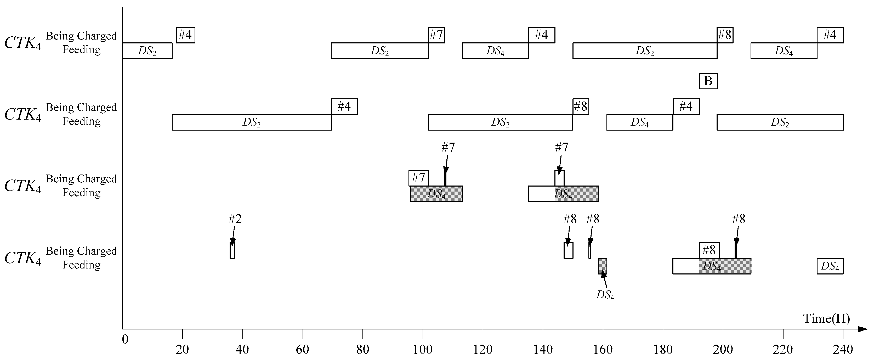
6. Industrial Case Study

This section presents a practical scenario of a refinery in China to show the application of the proposed method. The refinery has four distillers DS₁‒DS₄ with 10 charging tanks. A short-term schedule with 10-day scheduling horizon should be created three times a month to realize a target refining schedule. In this case, the refining schedule is shown in Figure 9, where #i denotes crude oil type #i, i Є {1, 2, …, 9}. The oil feeding rates for the distillers and maximal flow rate of the pipeline are f_ds1 = 323 tons/h, f_ds2 = 302 tons/h, f_ds3 = 625 tons/h, f_ds4 = 400 tons/h, and f_pmax = 1650 tons/h, respectively, which indicates f_pmax = f_ds1 + f_ds2 + f_ds3 + f_ds4. Note that distillers DS₁–DS₃ operate normally, while DS₄ is under maintenance at the beginning and will be put into operation at the beginning of the fifth day. The oil residency time for charging tanks is Ψ = 6 h, and the safety stock is σ = 1000 tons.

The initial state for the 10 charging tanks is shown in

Table 1. Initial state for the charging tanks.

Tank	Capacity (Ton)	Type of Oil Filled	Volume (Ton)
CTK1	16,000	Oil #1	9000
CTK2	16,000
CTK3	16,000	Oil #1	16,000
CTK4	16,000	Oil #3	5000
CTK5	16,000	Oil #3	16,000
CTK6	20,000
CTK7	20,000
CTK8	30,000	Oil #5	30,000
CTK9	30,000
CTK10	30,000	Oil #9	30,000

. Initially, CTK₁, CTK₄, and CTK₈ are feeding DS₁, DS₂, and DS₃, respectively. Note that, according to the refining schedule, the crude oil in CTK₁₀ is not to be processed during the scheduling horizon, and CTK₂ is under maintenance and cannot be used. Hence, there are three charging tanks ready for charging at the initial time. By checking the crude oil in the charging tanks and the refining schedule, we find that: (1) the pipeline needs to deliver 22,000 tons of oil type #1 from the storage tanks to the charging tanks for feeding DS₁ after the oil initially in CTK₁ and CTK₃ is used up; (2) DS₂ first processes the crude oil in CTK₄ and CTK₅, then these two charging tanks are ready for charging; (3) CTK₈ will be ready for charging after the oil initially in it is used up by feeding DS₃; and (4) CTK₉ is empty and free to be charged. Therefore, when DS₄ starts its operation at the beginning of the fifth day, the system has four distillers operating concurrently but only eight charging tanks are usable, i.e., there are not sufficient charging tanks in the refinery. Hence, the SCF mode has to be adopted for some time, and the system is scheduled with CTK₁ and CTK₃ being assigned to DS₁, CTK₄, and CTK₅ to DS₂, CTK₈, and CTK₉ to DS₃, CTK₆, to DS₄, and CTK₇ is used for the oil type switch if necessary. The PN model for this system is shown in Figure 10. Note that we do not model the charging tanks that are not available because they have no effect on finding a schedule. Also, in the model, CTK₇, which is used for oil type switches, is ignored for concision. In the model, {y, t_i2, t_i3, t_i4, t_i5, p_is, p_ic, p_i3}, i Є {1, 2, …, 10}, model CTK_i, while p_k and t_k, k Є {1, 2, 3, 4}, model DS_k and its distillation, respectively.

Based on the PN model shown in Figure 10, we code the scheduling method given by Proposition 8 and the evolution rules of the model to verify the proposed method. For this case study, we have μ ≤ min{ξ₁/α₁, ξ₃/α₁, ξ₄/α₂, ξ₅/α₂, ξ₈/α₃, ξ₉/α₃, ξ₆/α₄, ξ₅/α₁} = 8. To fully utilize the charging tanks, we set μ = 8. As f_ds2 < f_ds1 < f_ds3 holds, we have ϖ₁ = (μ × f_ds1 + μ × f_ds3 + μ × f_ds4 − 2f_pmax)/(f_ds4 + f_pmax) = 3.65. It can be verified that μ ≥ (ϖ₁ × f_ds4 + f_pmax)/f_ds4 = 7.78 and μ ≥ 2f_pmax/(f_ds1 + f_ds3 + f_ds4) = 2.45 hold. As the conditions in Proposition 8 are satisfied, we set Q = 1 and use the idle time of CTK₄ and CTK₅ to feed DS₄ under the normal mode for some time.

As the initial state is not exactly the same as required by Proposition 8, we can adjust the crude oil in the charging tanks by properly scheduling the oil delivering via the pipeline. Let τ_s = 0 h. According to Proposition 8, we schedule the pipeline as follows. When DS₄ starts its operation at time τ₁ = 96 h, one can use CTK₄ to feed DS₄ under the normal mode for some time. Thus, CTK₄ must be emptied at time τ₂ = τ₁ + Ψ = 102 h. Hence, we charge it with volume v₄ = (τ₂ − τ₀)×f_ds2 − 21,000 = 9804 tons of oil #4 only for feeding DS₂ when it is charged the first time. For this case, DS₁ has to process oil type #2 after 38,000 tons of oil type #1. We charge CTK₁ with 13,000 tons of oil type #1 and charge CTK₇ with 2504 tons of oil type #2 to realize the oil type switches.

To ensure the safety stock, we start charging CTK₆ with volume 1000 tons of oil #7 at time τ₃ = 95.4 h. By the above pipeline transportation schedule, at τ₁, the initial crude oil in charging tanks satisfies Condition (10). By following the scheduling method given by Proposition 8, the volumes of crude oil that should be transported from storage tanks to charging tanks for feeding distillers DS₁, DS₂, DS₃, and DS₄ are V₁ = μ × α₁ = 15,504 tons, V₂ = μ × α₂ = 14,496 tons, V₃ = μ × α₃ = 30,000 tons and V₄ = μ × α₄ = 19,200 tons, respectively. When oil type #7 is transported, it should first be charged into CTK₆ with volume v₁ = Ψ × f_pmax = 9900 tons, then into CTK₄ or CTK₅ with volume v₂ = ϖ₁ × f_ds1 = 8762 tons, and CTK₆ again with volume v₃ = V₄ − v₁ − v₂ = 538 tons. As DS₄ has to switch for processing different oil types, we charge CTK₆ with v₄ = 25,000 − V₄ = 4800 tons of oil type #7 and charge CTK₇ with v₅ = v₁ − v₄ = 5100 tons of oil type #8. When the oil #7 in CTK₆ for feeding DS₄ is used up at time τ₅ = 158.5 h and CTK₆ is emptied, CTK₇ starts feeding DS₄ with oil type #7 under the SCF mode. The sequence of charging the charging tanks and the time point for each event are shown in Figure 11.

Therefore, a schedule that realizes the refining schedule is obtained and the Gantt charts in Figure 11 and Figure 12 present the oil transportation from storage tanks to charging tanks and the detailed schedules of distiller feeding. Furthermore, the detailed schedule of charging tanks CTK₄, CTK₅, CTK₆, and CTK₇ for being charged and feeding distillers is presented in Figure 13, which clearly shows how the method given by Proposition 8 schedules the system to reduce the time during which DS₄ is fed by the charging tanks under the SCF mode. Since CTK₆ or CTK₇ is not charged or used to feed a distiller while CTK₄ or CTK₅ is feeding DS₄ for ϖ₁ × Ψ = 21.9 h > Ψ, CTK₆ or CTK₇ can feed DS₄ under the normal mode until it is charged by the pipeline again. Thus, we have Π = 3 × (2Ψ + ϖ₁ × α₄/f_pmax) = 51.9 h and δ = 51.9 ÷ (4 × 3 × 8 × 6) = 9% for the obtained schedule.

For this case, a detailed schedule that realizes the given refining schedule with all constraints considered is efficiently found. As pointed out in [21], if a mixed integer programming model is applied, the number of binary variables is huge and makes it extremely difficult or even impossible to solve such a large problem. Furthermore, the scheduling situation without sufficient charging tanks has not been discussed before, and the method proposed in [21,22] cannot be applied here as the number of charging tanks is much less than that required by the methods there. With the proposed method in this paper, a schedule can be easily created for a refinery without sufficient charging tanks such that the SCF mode is minimally used.

7. Discussion and Conclusions

Short-term scheduling for crude oil operations is a complex problem since a schedule needs to provide detailed activities such that all resource and process constraints are satisfied. Because of its NP-hard nature, there are no efficient techniques and software tools, and the scheduling job is still done manually. While scheduling a refinery without sufficient charging tanks, the limited number of charging tanks further complicates the problem. It is more challenging than a scheduling problem with sufficient charging tanks as the operational constraints and costs must be considered.

Instead of mathematical programming models, this paper studies the scheduling problem of crude oil operations by following a two-level architecture that solves the problem based on control theory. By this method, a detailed schedule is provided at the lower level to realize a refining schedule that is generated at the upper level. With this idea in mind, Wu et al. [21,22,24,25,26,27,28] built a hybrid PN model for the system to obtain a feasible schedule for crude oil operations. In these studies, generally, three charging tanks are needed for each distiller to find a schedule with the maximal production rate. Although their charging tank requirement can be satisfied for many refineries, there are refineries for which such a requirement is impossible. This is often the case when some charging tanks have to be maintained, or more distillers are installed without enough charging tanks being built. Hence, this work focuses on scheduling a refinery without sufficient charging tanks to solve such a practical problem. We build a new PN model for the system to describe the process accurately. Based on this model, a method that can schedule the system is proposed, and a schedule with the minimal usage of the SCF mode can be efficiently obtained via simple calculation.

This paper focuses on finding a schedule to realize a given refining schedule. When there are not sufficient charging tanks, it is better to create a refining schedule with the conditions given in this paper as constraints such that the obtained refining schedule is easy to realize. Our future work will take up this challenge.

References

1. Shah, N. Planning and Scheduling-Single-and Multisite Planning and Scheduling: Current Status and Future Challenges. AIChE Symp. Ser. 1998, 34, 75–90. [Google Scholar]
2. Moro, L.F.L. Process technology in the petroleum refining industry—Current situation and future trends. Comput. Chem. Eng. 2003, 27, 1303–1305. [Google Scholar] [CrossRef]
3. Kallestrup, K.B.; Lynge, L.H.; Akkerman, R.; Oddsdottir, T.A. Decision support in hierarchical planning systems: The case of procurement planning in oil refining industries. Decis. Support Syst. 2014, 68, 49–63. [Google Scholar] [CrossRef]
4. Pinto, J.M.; Moro, L.F.L. A planning model for petroleum refineries. Braz. J. Chem. Eng. 2000, 17, 575–585. [Google Scholar] [CrossRef]
5. Pelham, R.; Pharris, C. Refinery Operations and Control: A Future Vision; National Petroleum Refiners Association: Washington, DC, USA, 1996. [Google Scholar]
6. Shobrys, D.E.; White, D.C. Planning, scheduling and control systems: Why cannot they work together. Comput. Chem. Eng. 2002, 26, 149–160. [Google Scholar] [CrossRef]
7. Honkomp, S.J.; Lombardo, S.; Rosen, O.; Pekny, J.F. The curse of reality—Why process scheduling optimization problems are difficult in practice. Comput. Chem. Eng. 2000, 24, 323–328. [Google Scholar] [CrossRef]
8. Lee, H.; Pinto, J.M.; Grossmann, I.E.; Park, S. Mixed-Integer Linear Programming Model for Refinery Short-Term Scheduling of Crude Oil Unloading with Inventory Management. Ind. Eng. Chem. Res. 1996, 35, 1630–1641. [Google Scholar] [CrossRef]
9. Pinto, J.M.; Joly, M.; Moro, L.F.L. Planning and scheduling models for refinery operations. Comput. Chem. Eng. 2000, 24, 2259–2276. [Google Scholar] [CrossRef]
10. Saharidis, G.K.D.; Minoux, M.; Dallery, Y. Scheduling of loading and unloading of crude oil in a refinery using event-based discrete time formulation. Comput. Chem. Eng. 2009, 33, 1413–1426. [Google Scholar] [CrossRef]
11. Shah, N. Mathematical programming techniques for crude oil scheduling. Comput. Chem. Eng. 1996, 20, S1227–S1232. [Google Scholar] [CrossRef]
12. Jia, Z.Y.; Ierapetritou, M. Efficient short-term scheduling of refinery operations based on a continuous time formulation. Comput. Chem. Eng. 2004, 28, 1001–1019. [Google Scholar] [CrossRef]
13. Jia, Z.Y.; Ierapetritou, M.; Kelly, J.D. Refinery short-term scheduling using continuous time formulation: Crude-oil operations. Ind. Eng. Chem. Res. 2003, 42, 3085–3097. [Google Scholar] [CrossRef]
14. Mouret, S.; Grossmann, I.E.; Pestiaux, P. A Novel Priority-Slot Based Continuous-Time Formulation for Crude-Oil Scheduling Problems. Ind. Eng. Chem. Res. 2009, 48, 8515–8528. [Google Scholar] [CrossRef]
15. Mendez, C.A.; Grossmann, I.E.; Harjunkoski, I.; Kabore, P. A simultaneous optimization approach for off-line blending and scheduling of oil-refinery operations. Comput. Chem. Eng. 2006, 30, 614–634. [Google Scholar] [CrossRef]
16. Bai, L.P.; Wu, N.Q.; Li, Z.W.; Zhou, M.C. Optimal one-wafer cyclic scheduling and buffer space configuration for single-arm multicluster tools with linear topology. IEEE Trans. Syst. Man Cybern. Syst. 2016, 46, 1456–1467. [Google Scholar] [CrossRef]
17. Wu, N.Q.; Chu, F.; Chu, C.B.; Zhou, M.C. Petri net modeling and cycle time analysis of dual-arm cluster tools with wafer revisiting. IEEE Trans. Syst. Man Cybern. Syst. 2013, 43, 196–207. [Google Scholar] [CrossRef]
18. Wu, N.Q.; Zhou, M.C. Modeling, analysis and control of dual-arm cluster tools with residency time constraint and activity time variation based on Petri nets. IEEE Trans. Autom. Sci. Eng. 2012, 9, 446–454. [Google Scholar]
19. Wu, N.Q.; Zhou, M.C. Schedulability analysis and optimal scheduling of dual-arm cluster tools with residency time constraint and activity time variation. IEEE Trans. Autom. Sci. Eng. 2012, 9, 203–209. [Google Scholar]
20. Yang, F.J.; Wu, N.Q.; Qao, Y.; Zhou, M.C.; Li, Z.W. Scheduling of single-arm cluster tools for an atomic layer deposition process with residency time constraints. IEEE Trans. Syst. Man Cybern. Syst. 2017, 47, 502–516. [Google Scholar] [CrossRef]
21. Wu, N.Q.; Chu, F.; Chu, C.; Zhou, M.C. Short-term schedulability analysis of crude oil operations in refinery with oil residency time constraint using Petri nets. IEEE Trans. Syst. Man Cybern. Part C Appl. Rev. 2008, 38, 765–778. [Google Scholar] [CrossRef]
22. Wu, N.Q.; Chu, F.; Chu, C.; Zhou, M.C. Short-term schedulability analysis of multiple distiller crude oil operations in refinery with oil residency time constraint. IEEE Trans. Syst. Man Cybern. Part C Appl. Rev. 2009, 39, 1–16. [Google Scholar]
23. Wu, N.Q.; Zhou, M.C.; Chu, F. A Petri net-based heuristic algorithm for realizability of target refining schedule for oil refinery. IEEE Trans. Autom. Sci. Eng. 2008, 5, 661–676. [Google Scholar]
24. Wu, N.Q.; Zhou, M.C.; Li, Z.W. Short-term scheduling of crude-oil operations: Petri net-based control-theoretic approach. IEEE Robot. Autom. Mag. 2015, 22, 64–76. [Google Scholar] [CrossRef]
25. Wu, N.Q.; Chu, F.; Chu, C.B.; Zhou, M.C. Hybrid Petri net modeling and schedulability analysis of high fusion point oil transportation under tank grouping strategy for crude oil operations in refinery. IEEE Trans. Syst. Man Cybern. Part C 2010, 40, 159–175. [Google Scholar]
26. Wu, N.Q.; Chu, F.; Chu, C.B.; Zhou, M.C. Tank cycling and scheduling analysis of high fusion point oil transportation for crude oil operations in refinery. Comput. Chem. Eng. 2010, 34, 529–543. [Google Scholar] [CrossRef]
27. Wu, N.Q.; Chu, C.; Chu, F.; Zhou, M.C. Schedulability Analysis of Short-Term Scheduling for Crude Oil Operations in Refinery with Oil Residency Time and Charging-Tank-Switch-Overlap Constraints. IEEE Trans. Autom. Sci. Eng. 2011, 8, 190–204. [Google Scholar] [CrossRef]
28. Wu, N.Q.; Zhou, M.C.; Bai, L.P.; Li, Z.W. Short-term scheduling of crude oil operations in refinery with high fusion point oil and two transportation pipelines. Enterp. Inform. Syst. 2016, 10, 581–610. [Google Scholar] [CrossRef]
29. Wu, N.Q.; Bai, L.P.; Zhou, M.C. An efficient scheduling method for crude oil operations in refinery with crude oil type mixing requirements. IEEE Trans. Syst. Man Cybern. Syst. 2016, 46, 413–426. [Google Scholar] [CrossRef]
30. Wu, N.Q.; Bai, L.P.; Zhou, M.C.; Chu, F.; Mammar, S. A novel approach to optimization of refining schedules for crude oil operations in refinery. IEEE Trans. Syst. Man Cybern. Part C 2012, 42, 1042–1053. [Google Scholar]
31. Gribaudo, M.; Sereno, M.; Horv, A.; Bobbio, A. Fluid stochastic petri nets augmented with flush-out arcs: Modelling and analysis. Discret. Event Dyn. Syst. 2001, 11, 97–117. [Google Scholar] [CrossRef]
32. Horton, G.; Kulkarni, V.G.; Nicol, D.M.; Trivedi, K.S. Fluid stochastic petri nets: Theory, applications, and solution techniques. Eur. J. Oper. Res. 1998, 105, 184–201. [Google Scholar] [CrossRef]
33. Sanders, W.H.; Meyer, J.F. Stochastic Activity Networks: Formal Definitions and Concepts⋆. In Lectures on Formal Methods and Performance Analysis; Springer: Berlin, Germany, 2001; pp. 315–343. [Google Scholar]
34. Wang, J. Timed Petri Nets: Theory and Application; Springer: New York, NY, USA, 1998. [Google Scholar]
35. Zhou, M.C.; Venkatesh, K. Modeling, Simulation, and Control of Flexible Manufacturing Systems: A Petri Net Approach; World Scientific: Singapore, 1999. [Google Scholar]
Figure 1. Icons in the model.
Applsci 07 00564 g001
Figure 2. PN model for storage tanks.
Applsci 07 00564 g002
Figure 3. PN model for charging tanks.
Applsci 07 00564 g003
Figure 4. The PN model for the pipeline.
Applsci 07 00564 g004
Figure 5. PN model of the whole system.
Applsci 07 00564 g005
Figure 6. The PN model for a system with three charging tanks and two distillers.
Applsci 07 00564 g006
Figure 7. PN model for a system with four charging tanks and three distillers.
Applsci 07 00564 g007
Figure 8. PN model for a system with five charging tanks and three distillers.
Applsci 07 00564 g008
Figure 9. Refining schedule for the case study.
Applsci 07 00564 g009
Figure 10. PN model for the case study.
Applsci 07 00564 g010
Figure 11. Detailed schedule of oil transportation from storage tanks to charging tanks.
Applsci 07 00564 g011
Figure 12. Detailed schedule of distiller feeding.
Applsci 07 00564 g012
Figure 13. The schedule of charging tanks for being charged and feeding distillers.
Applsci 07 00564 g013