
An Improved Radio Resource Management with Carrier Aggregation in LTE Advanced


Abstract
:1. Introduction
2. Related Work
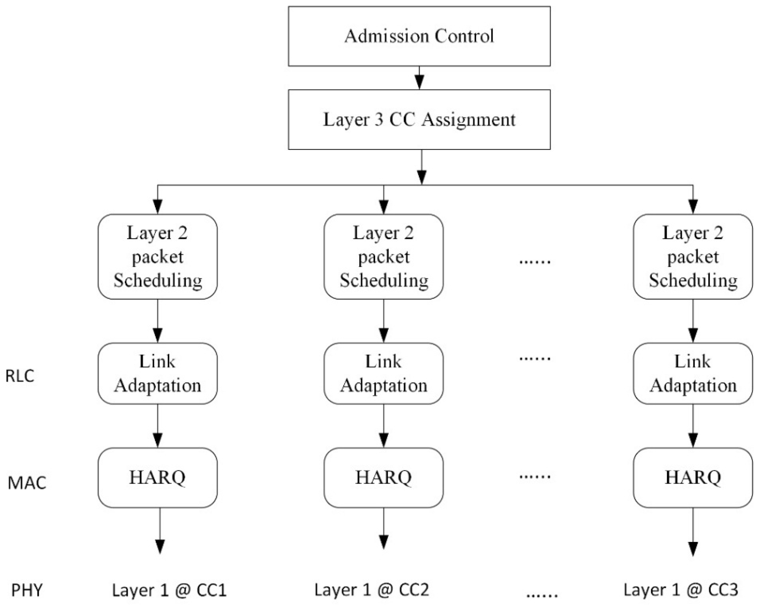
3. System Model
3.1. Problem Formulation
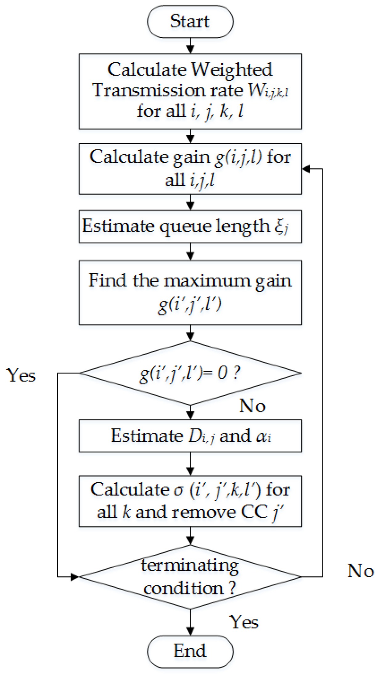
3.2. Proposed Greedy-Based Model
3.3. Computational Complexity
4. Results and Discussion
4.1. Simulation Settings
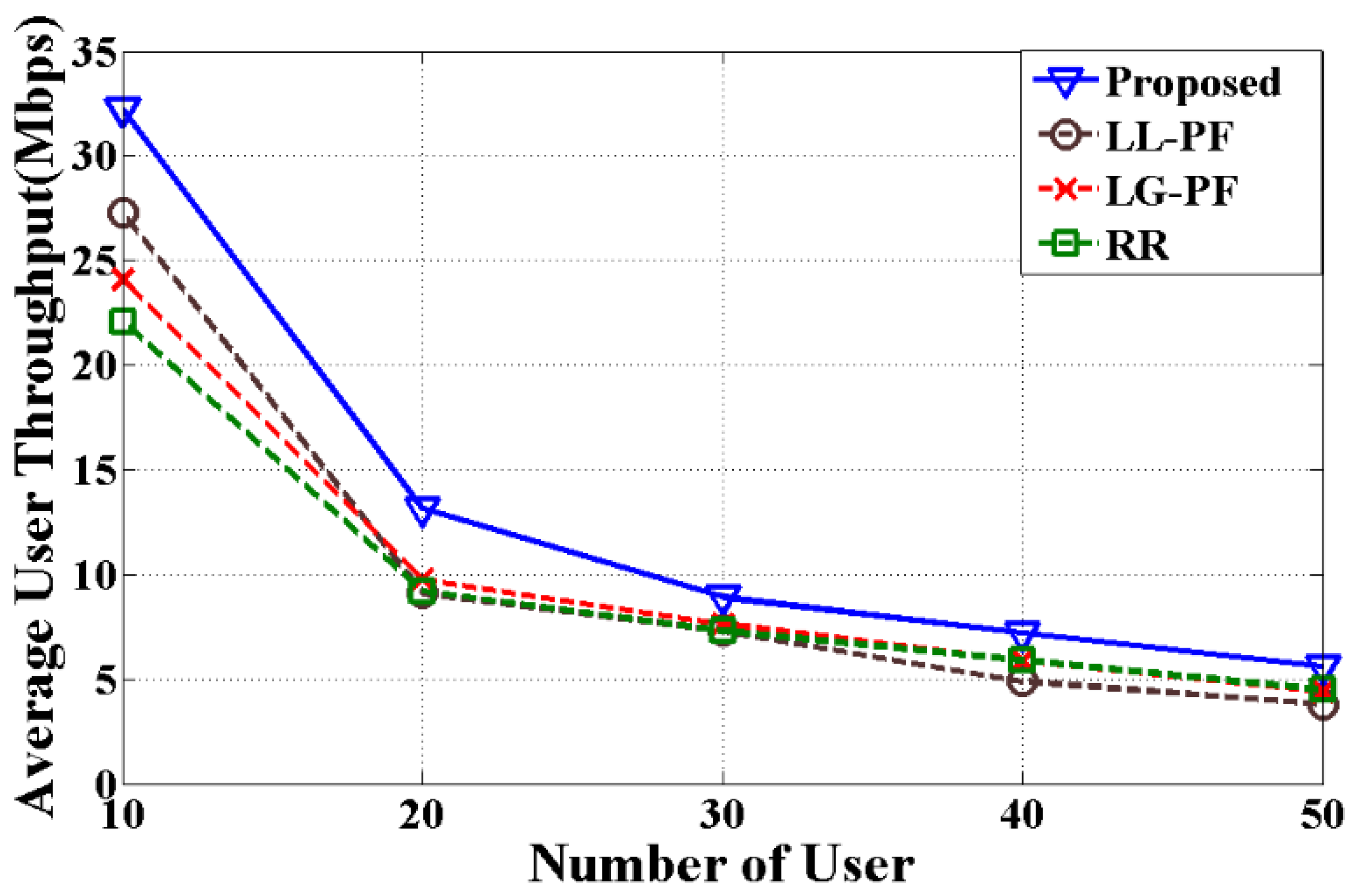
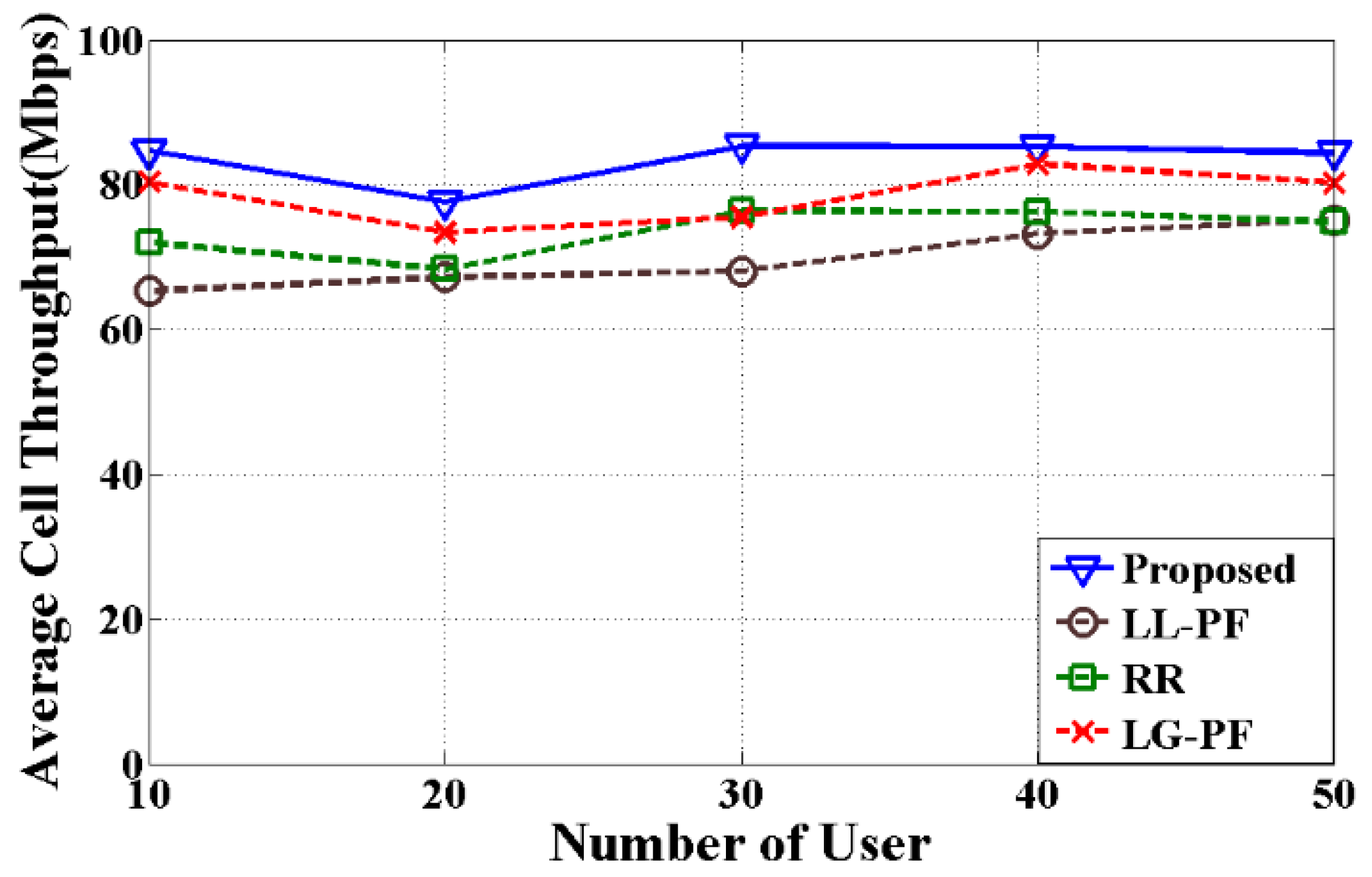
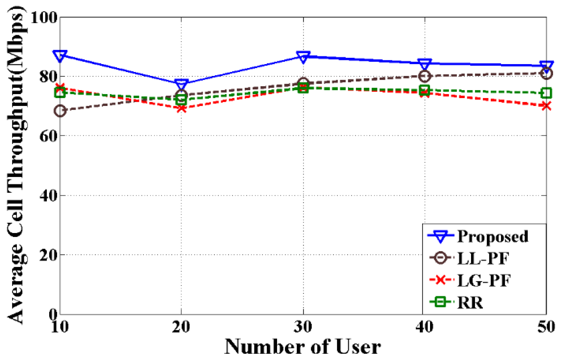
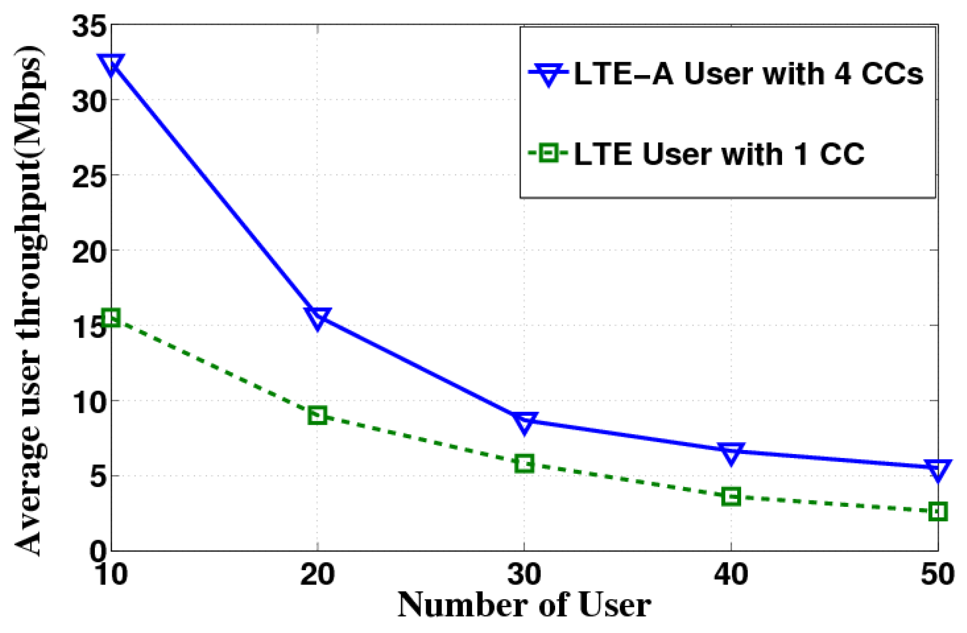
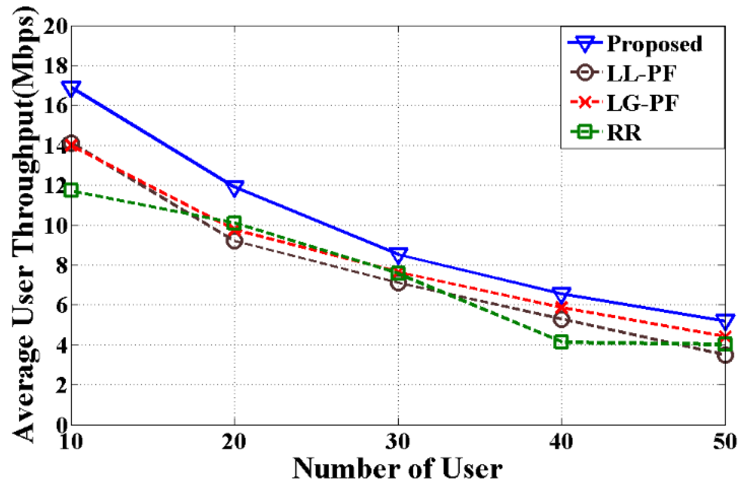
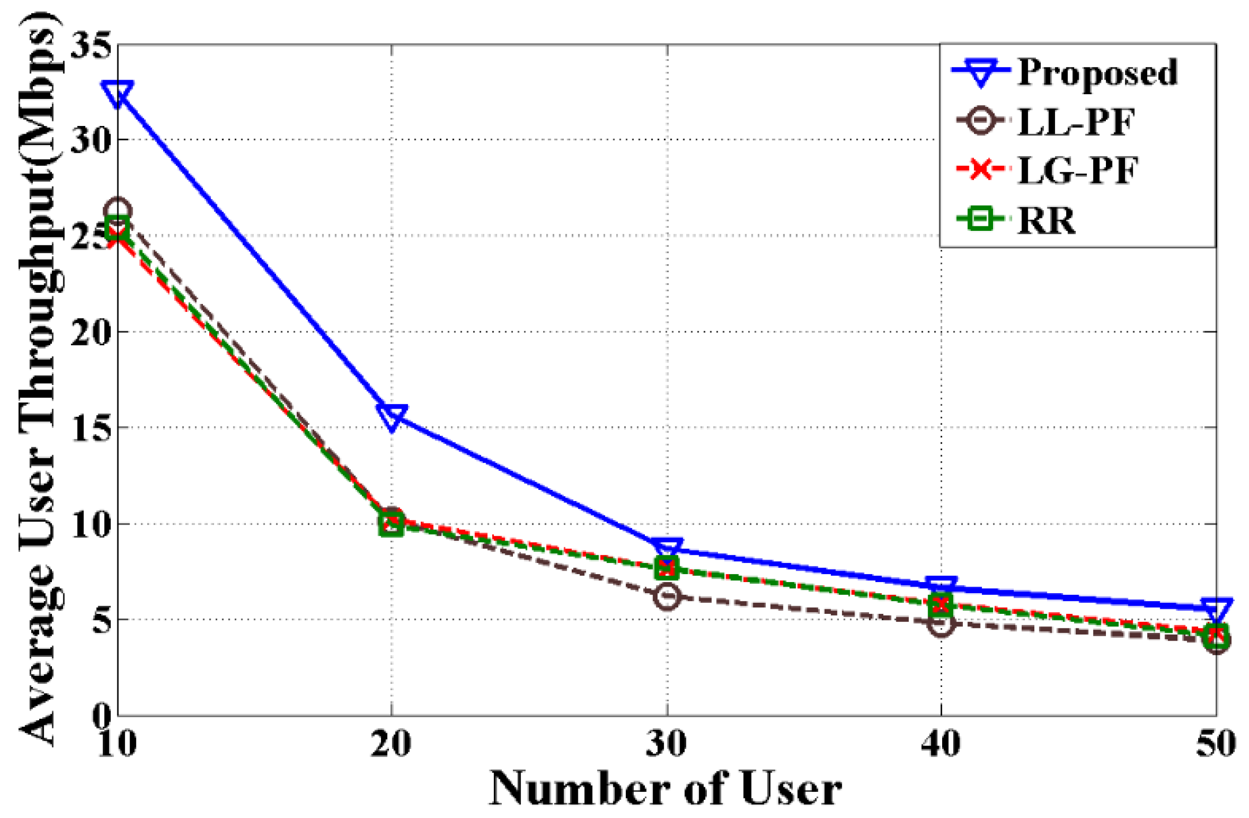
4.2. Simulation Results
5. Limitations and Future Work
6. Conclusions
Acknowledgments
Author Contributions
Conflicts of Interest
References
- Requirements for Further Advancements for Evolved Universal Terrestrial Radio Access (E-UTRA) (LTE-Advanced); Technical Report 36.913 V11.0.0; 3rd Generation Partnership Project (3GPP): Valbonne, France, September 2012.
- Evolved Universal Terrestrial Radio Access (E-UTRA) and Evolved Universal Terrestrial Radio Access Network (E-UTRAN); Overall Description; Stage 2, Technical Specification 36.300; 3rd Generation Partnership Project (3GPP): Valbonne, France, July 2012.
- LTE Carrier Aggregation Technology Development and Deployment Worldwide. White Paper. 4G Americas. October 2014. Available online: http://www.4gamericas.org/files/8414/1471/2230/4G_Americas_Carrier_Aggregation_FINALv1_0_3.pdf (accessed on 11 July 2016).
- Yuan, G.; Zhang, X.; Wang, W.; Yang, Y. Carrier aggregation for LTE-advanced mobile communication systems. IEEE Commun. Mag. 2010, 48, 88–93. [Google Scholar] [CrossRef]
- Rostami, S.; Arshad, K.; Rapajic, P. A joint resource allocation and link adaptation algorithm with carrier aggregation for 5G LTE-Advanced network. In Proceedings of the IEEE 22nd International Conference on Telecommunications (ICT), Sydney, Australia, 27–29 April 2015; pp. 102–106. [Google Scholar]
- Lee, H.; Vahid, S.; Moessner, K. A survey of radio resource management for spectrum aggregation in LTE-advanced. IEEE Commun. Surv. Tutor. 2014, 16, 745–760. [Google Scholar] [CrossRef]
- Wang, Y.; Pedersen, K.; Mogensen, P.E.; Sørensen, T.B. Resource allocation considerations for multi-carrier LTE-Advanced systems operating in backward compatible mode. In Proceedings of the IEEE 20th International Symposium on Personal, Indoor and Mobile Radio Communications, Toyko, Japan, 13–16 September 2009; pp. 370–374. [Google Scholar]
- Zhang, L.; Wang, Y.; Huang, L.; Wang, H.; Wang, W. QoS performance analysis on carrier aggregation based LTE-A systems. In Proceedings of the IET International Communication Conference on Wireless Mobile and Computing (CCWMC 2009), Shanghai, China, 7–9 December 2009; pp. 253–256. [Google Scholar]
- Zhang, L.; Liu, F.; Huang, L.; Wang, W. Traffic load balance methods in the LTE-Advanced system with carrier aggregation. In Proceedings of the IEEE International Conference on Communications, Circuits and Systems (ICCCAS), Chengdu, China, 28–30 July 2010; pp. 63–67. [Google Scholar]
- Wang, Y.; Pedersen, K.; Sørensen, T.B.; Mogensen, P.E. Utility maximization in LTE-advanced systems with carrier aggregation. In Proceedings of the IEEE 73rd Vehicular Technology Conference (VTC Spring), Budapest, Hungary, 15–18 May 2011; pp. 1–5. [Google Scholar]
- Ragaleux, A.; Baey, S.; Gueguen, C. Adaptive and Generic Scheduling Scheme for LTE/LTE-A Mobile Networks. Wirel. Netw. 2016, 22, 2753–2771. [Google Scholar] [CrossRef]
- Ferdosian, N.; Othman, M.; Ali, B.M.; Lun, K.Y. Multi-Targeted Downlink Scheduling for Overload-States in LTE Networks: Proportional Fractional Knapsack Algorithm with Gaussian Weights. IEEE Access 2017, 5, 3016–3027. [Google Scholar] [CrossRef]
- Ferdosian, N.; Othman, M.; Ali, B.M.; Lun, K.Y. Greedy–knapsack algorithm for optimal downlink resource allocation in LTE networks. Wirel. Netw. 2016, 22, 1427–1440. [Google Scholar] [CrossRef]
- Xenakis, D.; Passas, N.; Merakos, L.; Verikoukis, C. Mobility management for femtocells in LTE-advanced: Key aspects and survey of handover decision algorithms. IEEE Commun. Surv. Tutor. 2014, 16, 64–91. [Google Scholar] [CrossRef]
- Zorba, N.; Verikoukis, C. Joint uplink-downlink carrier aggregation scheme in LTE-A. In Proceedings of the IEEE 21st International Workshop on Computer Aided Modelling and Design of Communication Links and Networks (CAMAD), Toronto, ON, Canada, 23–25 October 2016; pp. 117–121. [Google Scholar]
- Zorba, N.; Verikoukis, C. Energy optimization for bidirectional multimedia communication in unsynchronized TDD systems. IEEE Syst. J. 2016, 10, 797–804. [Google Scholar] [CrossRef]
- Ramazanali, H.; Mesodiakaki, A.; Vinel, A.; Verikoukis, C. Survey of user association in 5G HetNets. In Proceedings of the 8th IEEE Latin-American Conference on Communications (LATINCOM), Medellin, Colombia, 16–18 November 2016; pp. 1–6. [Google Scholar]
- Andrews, M.; Kumaran, K.; Ramanan, K.; Stolyar, A.; Whiting, P.; Vijayakumar, R. Providing quality of service over a shared wireless link. IEEE Commun. Mag. 2001, 39, 150–154. [Google Scholar] [CrossRef]
- Stolyar, A.L.; Ramanan, K. Largest weighted delay first scheduling: Large deviations and optimality. Ann. Appl. Probab. 2001, 11, 1–48. [Google Scholar] [CrossRef]
- Ameigeiras, P.; Wigard, J.; Mogensen, P. Performance of the M-LWDF scheduling algorithm for streaming services in HSDPA. In Proceedings of the IEEE 60th Vehicular Technology Conference (VTC2004-Fall), Los Angeles, CA, USA, 26–29 September 2004; Volume 2, pp. 999–1003. [Google Scholar]
- Evolved Universal Terrestrial Radio Access (E-UTRA); Packet Data Convergence Protocol (PDCP); TS 25.323 V3.3.0; 3rd Generation Partnership Project (3GPP): Valbonne, France, April 2007.
- Ku, G.; Walsh, J.M. Resource allocation and link adaptation in LTE and LTE advanced: A tutorial. IEEE Commun. Surv. Tutor. 2014, 17, 1605–1633. [Google Scholar] [CrossRef]
- Lee, K.K.; Chanson, S.T. Packet loss probability for real-time wireless communications. IEEE Trans. Veh. Technol. 2002, 51, 1569–1575. [Google Scholar] [CrossRef]
- Meucci, F.; Cabral, O.; Velez, F.J.; Mihovska, A.; Prasad, N.R. Spectrum aggregation with multi-band user allocation over two frequency bands. In Proceedings of the IEEE Mobile WiMAX Symposium, Napa, CA, USA, 9–10 July 2009; pp. 81–86. [Google Scholar]
- Songsong, S.; Chunyan, F.; Caili, G. A resource scheduling algorithm based on user grouping for LTE-advanced system with carrier aggregation. In Proceedings of the International Symposium on Computer Network and Multimedia Technology (CNMT 2009), Wuhan, China, 18–20 December 2009; pp. 1–4. [Google Scholar]
- Liu, L.; Li, M.; Zhou, J.; She, X.; Chen, L.; Sagae, Y.; Iwamura, M. Component carrier management for carrier aggregation in LTE-advanced system. In Proceedings of the IEEE 73rd Vehicular Technology Conference (VTC Spring), Budapest, Hungary, 15–18 May 2011; pp. 1–6. [Google Scholar]
- Liao, H.-S.; Chen, P.-Y.; Chen, W.-T. An efficient downlink radio resource allocation with carrier aggregation in LTE-advanced networks. IEEE Trans. Mob. Comput. 2014, 13, 2229–2239. [Google Scholar] [CrossRef]
- Wang, Y.; Pedersen, K.; Sørensen, T.B.; Mogensen, P.E. Carrier load balancing and packet scheduling for multi-carrier systems. IEEE Trans. Wirel. Commun. 2010, 9, 1780–1789. [Google Scholar] [CrossRef]
- General Packet Radio Service (GPRS) enhancements for Evolved Universal Terrestrial Radio Access Network (E-UTRAN) Access; TS 23.401 V8.1.0; 3rd Generation Partnership Project (3GPP): Valbonne, France, April 2008.
- Nasralla, M.M.; Hewage, C.T.; Martini, M.G. Subjective and objective evaluation and packet loss modeling for 3d video transmission over LTE networks. In Proceedings of the IEEE International Conference on Telecommunications and Multimedia (TEMU), Heraklion, Crete, Greece, 28–30 July 2014; pp. 254–259. [Google Scholar]
- Anchora, L.; Canzian, L.; Badia, L.; Zorzi, M. A characterization of resource allocation in LTE systems aimed at game theoretical approaches. In Proceedings of the 15th IEEE International Workshop on Computer Aided Modeling, Analysis and Design of Communication Links and Networks (CAMAD), Miami, FL, USA, 3–4 December 2010; pp. 47–51. [Google Scholar]
- Rupp, M.; Schwarz, S.; Taranetz, M. The Vienna LTE-Advanced Simulators; Springer: Berlin, Germany, 2016. [Google Scholar]
- Institute of Telecommunications, Vienna University of Technology. Vienna LTE-A Simulators. Available online: https://www.nt.tuwien.ac.at/research/mobile-communications/vienna-lte-a-simulators/ (accessed on 22 April 2016).
- Evolved Universal Terrestrial Radio Access (E-UTRA); Physical Layer Procedures; Technical Specification 36.213 V11.0.0; 3rd Generation Partnership Project (3GPP): Valbonne, France, September 2012.
- Jain, R.; Chiu, D.-M.; Hawe, W.R. A Quantitative Measure of Fairness and Discrimination for Resource Allocation in Shared Computer System; Eastern Research Laboratory, Digital Equipment Corporation: Hudson, MA, USA, 1984; Volume 38. [Google Scholar]


| CC Selection Method | Packet Scheduler | Characteristics | Reference |
|---|---|---|---|
| Random selection with load balancing | Cross-CC PF |
| [7] |
| Circular selection | RR |
| [9] |
| Inter-band carrier switch | PF |
| [24] |
| Lowest path loss | User grouping PF (UG-PF) |
| [25] |
| Absolute and Relative policy | PF |
| [26] |
| Largest gain | PF |
| [27] |
| Least load | PF |
| [28] |
| Symbol | Definition |
|---|---|
| i | User, i ϵ Q = {1, …., Q} |
| j | CC, j ϵ R = {1, …., R} |
| k | RB, k ϵ S = {1, …., S} |
| l | MSC index, l ϵ T = {1, …., T} |
| m | Maximum number of CC can be assigned to a user |
| t | Time (TTI index) |
| ψi,j,k,l | A variable to denote whether or not CC j, RB k and MSC l is assigned to user i |
| Wi,j,k,l | Weighted transmission rate of user i, CC j, RB k, and MSC l |
| Di,j | Head of line delay of user i, CC j |
| ξj | Queue length of CC j |
| δi | Probability of packet loss of user i |
| Ω (j, k) | Transmission rate of user currently being allocated with CC j and RB k |
| g (i, j, l) | The gain after assigning CC j and MSC l to user i |
| σ (i, j, k, l) | Weighted transmission rate metric with packet loss and delay |
| Application | Delay Threshold in ms | Priority Level |
|---|---|---|
| Real time gaming | 50 | 3 |
| Live video streaming | 100 | 7 |
| Conversational voice | 100 | 2 |
| HTTP, FTP | 300 | 6 |
| Algorithm 1 Proposed method |
| 1: Ω (j, k) = 0 for all CC j and RB k |
| 2: Calculate Wi,j,k,l for all i ϵ Q, j ϵ R, k ϵ S, l ϵ T |
| 3: repeat |
| 4: Calculate gain g (i, j, l) for all i, j and l |
| 5: Calculate Queue length ξj for each CC j |
| 6: (i′, j′, l′) = argmax i ϵ Q, j ϵ R,lϵ T g (i, j, l)/ξj |
| 7: if g (i′, j′, l′) = 0 |
| 8: go to line 21; otherwise |
| 9: Assign CC j′ to user i′ with MSC l′ |
| 10: Calculate Head of Line Delay Di′, j′ of user i′ for CC j′ |
| 11: Estimate the variable αi′ of user i′ |
| 12: for each k ϵ S do |
| 13: σ (i′, j′, k, l′) = Wi′, j′, k, l′ * αi’ * Di′, j′ |
| 14: if σ (i′, j′, k, l′) > Ω (j′, k) then |
| 15: Assign RB k of CC j′ to user i′ |
| 16: Ω (j′, k) = σ (i′, j′, k, l′) |
| 17: end if |
| 18: end for |
| 19: Remove CC j′ associated with user i′ |
| 20: end if |
| 21: until reach any terminating condition |
| Parameters | Values |
|---|---|
| Operating frequency band | 900 MHz and 2100 MHz |
| Total bandwidth | 40 MHz (4 × 10 MHz) |
| Scenario | Urban (Random user deployment) |
| Number of users | 10, 20, 30, 40, 50 |
| User speed | 5 kmph |
| Scheduling algorithm | Proposed algorithm, LL-PF, LG-PF, RR |
| MSC index | 29 available MSCs as in 3GPP [34] |
| eNodeB power transmission | 46 dBm |
| Thermal noise density of the user | −174 dBm |
| Simulation time | 1000 TTI |
| Traffic model | Video, VoIP, HTTP |
| Operating frequency band | 900 MHz and 2100 MHz |
| Total bandwidth | 40 MHz (4 × 10 MHz) |
| Scenario | Urban (Random user deployment) |
| Traffic Model | Algorithm | Average User Throughput (%) | Average Cell Throughput (%) |
|---|---|---|---|
| Video | LG-PF | 16.73 | 13.43 |
| LL-PF | 28.30 | 19.86 | |
| RR | 32.51 | 6.38 | |
| HTTP | LG-PF | 26.82 | 14.70 |
| LL-PF | 35.62 | 10.48 | |
| RR | 31.29 | 12.64 | |
| VoIP | LG-PF | 27.95 | 16.87 |
| LL-PF | 39.40 | 31.81 | |
| RR | 29.71 | 17.14 |
© 2017 by the authors. Licensee MDPI, Basel, Switzerland. This article is an open access article distributed under the terms and conditions of the Creative Commons Attribution (CC BY) license (http://creativecommons.org/licenses/by/4.0/).
Share and Cite
Chayon, H.R.; Dimyati, K.; Ramiah, H.; Reza, A.W. An Improved Radio Resource Management with Carrier Aggregation in LTE Advanced. Appl. Sci. 2017, 7, 394. https://doi.org/10.3390/app7040394
Chayon HR, Dimyati K, Ramiah H, Reza AW. An Improved Radio Resource Management with Carrier Aggregation in LTE Advanced. Applied Sciences. 2017; 7(4):394. https://doi.org/10.3390/app7040394
Chicago/Turabian StyleChayon, Hasibur Rashid, Kaharudin Dimyati, Harikrishnan Ramiah, and Ahmed Wasif Reza. 2017. "An Improved Radio Resource Management with Carrier Aggregation in LTE Advanced" Applied Sciences 7, no. 4: 394. https://doi.org/10.3390/app7040394
APA StyleChayon, H. R., Dimyati, K., Ramiah, H., & Reza, A. W. (2017). An Improved Radio Resource Management with Carrier Aggregation in LTE Advanced. Applied Sciences, 7(4), 394. https://doi.org/10.3390/app7040394