Adaptive Feature Extraction of Motor Imagery EEG with Optimal Wavelet Packets and SE-Isomap

Abstract

Motor imagery EEG (MI-EEG), which reflects one’s active movement intention, has attracted increasing attention in rehabilitation therapy, and accurate and fast feature extraction is the key problem to successful applications. Based on wavelet packet decomposition (WPD) and SE-isomap, an adaptive feature extraction method is proposed in this paper. The MI-EEG is preprocessed to determine a more effective time interval through average power spectrum analysis. WPD is then applied to the selected segment of MI-EEG, and the subject-based optimal wavelet packets (OWPs) with top mean variance difference are obtained autonomously. The OWP coefficients are further used to calculate the time-frequency features statistically and acquire the nonlinear manifold structure features, as well as the explicit nonlinear mapping, through SE-isomap. The hybrid features are obtained in a serial fusion way and evaluated by a k-nearest neighbor (KNN) classifier. The extensive experiments are conducted on a publicly available dataset, and the experiment results of 10-fold cross-validation show that the proposed method yields relatively higher classification accuracy and computation efficiency simultaneously compared with the commonly-used linear and nonlinear approaches.

1. Introduction

A brain computer interface (BCI) system is an emerging technology that is regarded as a new way for the human brain to control external devices without the neural pathway [1]. People can control external devices by imagining the relevant action. Currently, BCI-based rehabilitation therapy is focused mainly on the recognition of motor imagery EEG (MI-EEG) [2,3,4] that is collected when a subject performs a specific motion imagination. However, the high dimension of the MI-EEG signal, which leads to high computational cost, usually brings an obstacle to the implementation of the on-line recognition algorithm and adversely affects the classification accuracy of MI-EEG. Therefore, how to effectively extract the low-dimensional representation hidden in the high-dimensional dataset has been a hotspot in the BCI and machine learning field in recent years [5,6,7]. To solve the computational complexity and data storage problem caused by the high dimension of signals, many dimensionality reduction methods have been used in traditional BCI technology, such as principal component analysis (PCA), independent components analysis (ICA) and multidimensional scaling (MDS). PCA assumes that the samples are not correlated, and its main idea is to calculate a group of new features arranged in the descending order of importance from the original ones that are linear combinations [8]; ICA is similar to PCA, except that the components are designed to be independent of each other; and MDS is an unsupervised data dimensionality reduction method, in which efforts are taken to find the low dimensional embedding that best preserves the pair-wise distances between the original data points [9]. All of these methods have been widely used in visualization and feature extraction, for they are well understood and easy to implement. Unfortunately, they have a common inherent limitation, i.e., they are all linear methods, while MI-EEG can be regarded as the output of the brain, which contains much nonlinear geometry information [10]. The features extracted by the methods will not be adequate and effective [11], and the classification accuracy will also be affected. The manifold learning theory provides a new way to solve the problem.

In 2000, two nonlinear dimensionality reduction methods, isomap and locally linear embedding (LLE) algorithms, were proposed by Tenenbaum et al. [12] and Roweis et al. [13]. They were published in the famous “Science” journal and created a new genre of manifold learning (ML) in machine learning. ML assumes that the high-dimensional spatial data observed in the real world are usually generated by a relatively small number of degrees of freedom [12], and the data can be embedded in a lower dimensional space according to its preserved geometry [14]. Since then, ML has begun to emerge in the BCI field. Sadatnejad et al. [15] proposed a new kernel function method for the symmetric positive definite (SPD) matrix of the MI-EEG signal, and the isomap algorithm was applied to the dimension reduction of the SPD matrix. The KNN classifier was used to classify features, and the experiments yielded a promising result when compared with the most popular manifold learning methods, as well as the common spatial pattern (CSP) technique; Mirsadeghi et al. [16] calculated the power, covariance and a series of the entropy of the EEG signal to obtain its original features, and the LLE algorithm was implemented to reduce the feature dimension. The depth of anesthesia was estimated by quadratic discriminant analysis, and the average classification rate was 88.4%. Krivov et al. [10], who came from the Kharkevich Institute, proposed a method to reduce the dimension of the covariance matrix of the MI-EEG signal by using the isomap algorithm, and the concept of Riemannian geometry was introduced. The useful information hidden in MI-EEG was explored from the perspective of spatial structure, and the classification accuracy is as good as the state-of-the-art CSP algorithm. These manifold learning methods have achieved surprising results in the research of MI-EEG. However, they cannot obtain the explicit mapping relationship from the high-dimensional space to the low-dimensional space while acquiring low-dimensional embedding representations. Therefore, it is impossible to directly extract the features from a new sample when carrying out a pattern recognition task. To solve the problem and enhance the resolvability of multi-class datasets, Li et al. [14,17] extended the original isomap and proposed the supervised explicit isomap (SE-isomap) algorithm, in which the geodesic distance matrix is calculated with respect to the class label information, and MDS with explicit transformation is adopted instead of the classical MDS used in the isomap. It is regretful that the SE-isomap has not been applied to the feature extraction of the MI-EEG signal.

As we know, MI-EEG is non-stationary and time varying, and it has a clear time-frequency distribution. Both wavelet transform (WT) and wavelet packet decomposition (WPD) are common and effective time-frequency analysis methods [18,19,20], and WPD, which is an extension of WT, can simultaneously decompose the signal into high-frequency components and low-frequency components; thus, the range of time-frequency analysis is broadened, and more time-frequency domain information embedded in a signal is then obtained. Additionally, WPD has been proven to be able to obtain the dynamic characteristics of a signal effectively [21]. Consequently, WPD has attracted increasing attention from the BCI field in recent years. Yang et al. [19] applied WPD to extracting the time-frequency features of MI-EEG, and the wavelet packet coefficients were input to the CSP algorithm to obtain a set of six-dimensional eigenvectors. The probabilistic neural network (PNN) was further used to classify the features, and the average recognition accuracy is 88.66%; Luo et al. [22] extracted the MI-EEG time-frequency information by using WPD and then applied the dynamic frequency feature selection (DFFS) algorithm to select the sub-WPD coefficients associated with the imaging task. The random forests algorithm was used to evaluate the features, and the average classification accuracy from nine different subjects reached 84.06%. It is obvious that WPD has been playing an important role in the feature extraction of MI-EEG. However, the frequency range of each wavelet packet subspace (WPS) is relatively fixed; the same WPSs are selected for different subjects by using the above WPD-based methods, namely as the time-frequency features; the WPD coefficients are covered by the same frequency ranges. This is not good for the extraction of subject-specific features and results in the poor adaptability of WPD-based feature extraction methods. In this paper, an adaptive feature extraction method is proposed for MI-EEG based on WPD and SE-isomap. The optimal wavelet packets (OWPs), reflecting the subject-based features, are autonomously selected, and the coefficients of OWPs are utilized to statistically calculate time-frequency features. In the meantime, SE-isomap is applied to obtain the nonlinear manifold structure features, as well as the explicit nonlinear mapping. The combined features show the perfect performance in classification accuracy and computation efficiency.

The rest of the paper is organized as follows: In Section 2, the basic principles of WPD, the SE-isomap algorithm and explicit-MDS are briefly introduced. Section 3 describes the feature extraction method with WPD and SE-isomap algorithm in detail. In the following section, extensive experiments are conducted on a publicly available dataset. Section 5 concludes the paper.

2. Primary Theory

2.1. Wavelet Packet Decomposition

The sampled signal in WT will be passed through the low-pass and high-pass filters to obtain the corresponding results. Each result is considered as a sub-space; however, only the low-pass filter results will be regarded as the input of the next step and then get another layer of low-pass and high-pass filtered results [23]. Different from the WT, WPD will transform the results of low-pass and high-pass filters further; therefore, the results of wavelet packet transform can be regarded as a complete binary tree whose root node is the original signal, and the sub-nodes of the next layer are the results of WT [20,24]. A three-level sub-band tree is shown in Figure 1, where s(0,0) represents the initial space of the dataset, s(j,n) denotes the decomposed WPS, j represents the number of decomposed levels and n represents the index of the subspace at the j-th level. The k-th WPD coefficient of the n-th wavelet packet at the j-th level can be expressed as:

$$d_j^n\left(k\right)=\{\begin{array}{c}{\displaystyle \sum _n}{h}_0\left(m-2k\right)d_{j-1}^{n/2}\left(m\right)\mathrm{if}n\mathrm{is}\mathrm{even}\\ {\displaystyle \sum _n}{h}_1\left(m-2k\right)d_{j-1}^{\left(n-1\right)/2}\left(m\right)\mathrm{if}n\mathrm{is}\mathrm{odd}\end{array}$$

(1)

where $h_0\left(k\right)$ and $h_1\left(k\right)$ are a pair of quadrature mirror filters that are irrelevant to the levels, and the relationship between them is as follows:

$$h_1\left(k\right)={\left(-1\right)}^{1-k}{h}_0\left(1-k\right)$$

(2)

After that, the decomposition coefficient of the j-th layer can be obtained by iteratively calculating the coefficients of the (j − 1)-th layer.

The frequency range corresponding to the subspace s(j,n) is [$\frac{n{f}_{\mathrm{s}}}{2^{j+1}},\left(n+1\right)f_{\mathrm{s}}/2^{j+1}$], where $f_{\mathrm{s}}$ represents the sampling frequency.

The energy of a signal is decomposed into the time-frequency domain by WPD, and it can be reflected by the unit value of WPD coefficients. Because of the perfect performance of WPD, it is superior to other methods in dealing with the typical non-stationary signals, like MI-EEG [25].

2.2. SE-Isomap Algorithm

As an extension of original isomap algorithm, SE-isomap [17] is able to effectively exploit the label information of the training samples to aggregate the samples belonging to the same class and disperse others properly; therefore, the separability of the samples is enhanced and the explicit mapping of the samples from the high-dimensional space to the target space is obtained, which significantly shortens the time of the feature extraction procedure. The basic principle is as follows:

Suppose that the dataset X contains two types of samples $C_b\left(b=1,2\right)$, namely $\mathit{X}=C_1{\displaystyle \cup }{C}_2,C_b=\left\{x_i^b,x_i^b\in R^D,i=1,2,\dots ,N_b\right\}$, where $N_b$ represents the number of samples in the $C_b$ class dataset, and D denotes the dimension of the observation space where the dataset is located. Assuming that the intrinsic dimension of the manifold embedded in the dataset is d $\left(d\ll D\right)$, the SE-isomap algorithm usually consists of three steps:

(1)

Constructing the intra-class distance matrix: Calculate the k-nearest neighbors for each sample ${\mathit{x}}_i\left(i=1,2,\dots ,N_b\right)$ in class $C_b\left(b=1,2\right)$ to get $x_i^1,x_i^2,\dots ,x_i^k$ and regard as $\mathit{N}\left({\mathit{x}}_i\right)$. Then, the neighborhood graph $G_b\left(V,E\right)$ is constructed with the sample $x_i$ as the vertex and the Euclidean distance $d\left({\mathit{x}}_i,{\mathit{x}}_j\right)$ between the sample as the edge. The shortest path distance in the neighbor graph $G_b\left(V,E\right)$ between the two vertexes will be regarded as an approximation of the geodesic distance between two corresponding samples. For convenience of expression, the geodesic distance $g\left({\mathit{x}}_i,{\mathit{x}}_j\right)$ is simplified to $g_{ij}$, then the geodesic distance between ${\mathit{x}}_i$ and ${\mathit{x}}_j$ is as follows:

$$g_{ij}=g\left({\mathit{x}}_i,{\mathit{x}}_j\right)=\{\begin{array}{c}{g}_{ij}\forall x_i\in N\left({\mathit{x}}_j\right)\mathrm{or}{x}_j\in N\left({\mathit{x}}_i\right)\\ \underset{k}{\min }\left\{g_{ij},g_{ik}+g_{kj}\right\}\mathrm{elsewise}\end{array}$$

(3)

Then, the intra-class geodesic distance matrix ${\mathit{G}}_{bb}={\left(g_{ij}\right)}_{N_b\times N_b}$ is constructed according to the approximate geodesic distance between two arbitrary points.

(2)

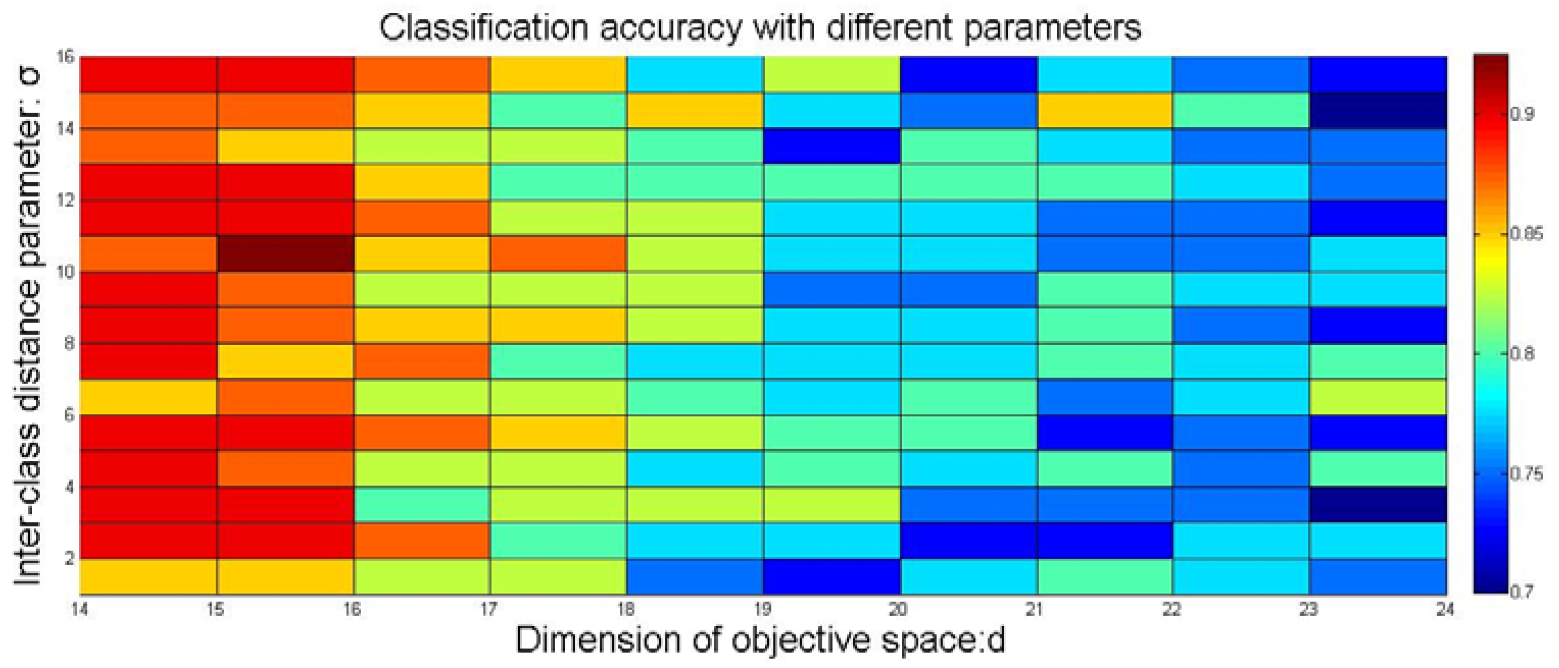
Constructing the global discriminative distance matrix: Calculate the inter-class geodetic distance $g^{*}\left({\mathit{x}}_i,{\mathit{x}}_j\right)$ between any two samples when ${\mathit{x}}_i\in C_1\mathrm{and}{\mathit{x}}_j\in C_2$, and the computational equation is as follows:

$$g^{*}\left({\mathit{x}}_i,{\mathit{x}}_j\right)=g\left({\mathit{x}}_i,x_{i^{*}}\right)+d\left(C_1,C_2\right)+g\left({\mathit{x}}_{j^{*}},{\mathit{x}}_j\right)$$

(4)

where the sample pairs $\left({\mathit{x}}_{i^{*}},{\mathit{x}}_{j^{*}}\right)=\arg \underset{\forall p\in C_1,q\in C_2}{\min }d\left(p,q\right)$; $\underset{\forall p\in C_1,q\in C_2}{\min }d\left(p,q\right)$ denotes the shortest euclidean distance between class $C_1$ and class $C_2$; $g\left({\mathit{x}}_i,{\mathit{x}}_{i^{*}}\right)$ and $g\left({\mathit{x}}_{j^{*}},{\mathit{x}}_j\right)$ denote the intra-class geodesic distance between ${\mathit{x}}_i$ and ${\mathit{x}}_{i^{*}}$, ${\mathit{x}}_{j^{*}}$ and ${\mathit{x}}_j$, respectively. In general, the calculative strategy of inter-class geodesic distance $d\left(C_1,C_2\right)$ is different when applied to different experimental tasks. Equation (5) is chosen for visualization to ensure the authenticity of the structure of the dataset:

$$d\left(C_1,C_2\right)=\underset{\forall {\mathit{x}}_i\in C_1,\forall {\mathit{x}}_j\in C_2}{\min }d\left({\mathit{x}}_i,{\mathit{x}}_j\right)$$

(5)

When the classify experiment is implemented to enhance the separability, Equation (6) will be taken into consideration:

$$d\left(C_1,C_2\right)=\sigma \underset{l=1,2}{\max }\left\{\underset{{\mathit{x}}_i,{\mathit{x}}_j\in C_l}{\max }\left\{d_{\mathit{G}}\left({\mathit{x}}_i,{\mathit{x}}_j\right)\right\}\right\}$$

(6)

The inter-class distance parameter $\sigma$ is used to balance the fidelity of visualization and the separability of data. Then, the inter-class distance matrix can be denoted as ${\mathit{G}}_{12}={(g_{ij}^{*})}_{N_1\times N_2}$. Finally, the global geodesic distance matrix G representing the distance between any individual sample points is constructed as:

$$\mathit{G}=\left(\begin{array}{c}{\rho }_1{\mathit{G}}_{11}{\mathit{G}}_{12}\\ {\mathit{G}}_{21}{\rho }_2{\mathit{G}}_{22}\end{array}\right)$$

(7)

where ${\mathit{G}}_{11}$ and ${\mathit{G}}_{22}$ are the intra-class geodesic distance matrices of class $C_1$ and class $C_2$, respectively, ${\mathit{G}}_{12}$ and ${\mathit{G}}_{21}$ are the inter-class geodesic distance matrices of the samples belong to different classes and ${\mathit{G}}_{12}={\mathit{G}}_{21}^{\mathrm{T}}$ and parameters $0<{\rho }_1\mathrm{and}{\rho }_2<1$ are used to reduce the intra-class distance properly for the reason that the gather effect will be reinforced.

(3)

Utilizing the explicit-MDS algorithm to obtain the low-dimensional embedding expression and the corresponding mapping relation of the dataset: The explicit-MDS algorithm is applied to obtain the low-dimensional expression $y\in R^d$ and explicit mapping matrix ${\mathit{W}}_{\mathrm{opt}}$.

2.3. Explicit-MDS

Utilizing the explicit-MDS algorithm on the global geodesic distance matrix G, the corresponding mapping $\mathit{f}=R^D\to R^d$ can be obtained while obtaining the low-dimensional representation of the data, where $\mathit{f}={\left(f_1,f_2,\dots ,f_d\right)}^{\mathrm{T}}$. For any $\mathit{x}\in R^D$,

$$y=f\left(x\right)={\mathit{W}}^{\mathrm{T}}\mathit{\Phi }\left(x\right)$$

(8)

where $\mathit{W}\in R^{r\times d}$ denotes the weight coefficient matrix, $\mathit{\Phi }\left(\mathit{x}\right)={\left({\mathit{\Phi }}_1\left(\mathit{x}\right),{\mathit{\Phi }}_2\left(x\right),\dots ,{\mathit{\Phi }}_r\left(\mathit{x}\right)\right)}^{\mathrm{T}}$ is the column vector, $\mathrm{y}\in R^d$ is the optimal low-dimensional expression of the original data in the target space and ${\mathit{\Phi }}_j:R^D\to R^1\left(j=1,\dots ,r\right)$ is a set of non-liner basis functions. Here, the radial basis function (RBF) is selected to construct the functions:

$${\mathit{\Phi }}_j\left({\mathit{x}}_i\right)=\exp \left\{-\frac{{\parallel {\mathit{x}}_i-{\mathit{c}}_j\parallel }^2}{\beta }\right\}$$

(9)

where ${\mathit{c}}_j\left(j=1,2,\dots ,\mathrm{l}\right)$ denotes the centers of the RBF ${\mathit{\Phi }}_j(·)$ and $\beta$ denotes the bandwidth parameter determined by the mean distance of the dataset. Correspondingly, the objective function is constructed as:

$$\epsilon \left(\mathit{W}\right)={\displaystyle \sum }_{i=1}^n{\displaystyle \sum }_{j=1}^l{\left(g_{ij}-q_{ij}\left(\mathit{W}\right)\right)}^2$$

(10)

where $q_{ij}\left(\mathit{W}\right)=\parallel {\mathit{W}}^{\mathrm{T}}\left({\mathit{\Phi }}_i-{\mathit{\Phi }}_j\right)\parallel$ denotes the pairwise Euclidean distance between the constructed points in the target space after dimensionality reduction. The problem is transformed to obtain the optimal weight matrix W that can minimize the objective function. An iterative optimization algorithm is used to resolve the problem of least squares on W. The algorithm steps are as follows:

• Step 1. Let t = 0, and initialize the weight matrix ${\mathit{W}}^{\left(t\right)}$;
• Step 2. Let V = ${\mathit{W}}^{\left(t\right)}$;
• Step 3. Update ${\mathit{W}}^{\left(t+1\right)}=\arg \underset{\mathit{W}}{\min }{\epsilon }_{\mathrm{m}}\left(\mathit{W},\mathit{V}\right)$; ${\mathit{W}}^{\left(t+1\right)}$ is the solution of minimization problem ${\epsilon }_{\mathrm{m}}\left(\mathit{W},\mathit{V}\right)$, and $\mathit{W}={\mathit{A}}^{+}\mathit{B}\left(\mathit{V}\right)\mathit{V}$, where:

  $$\mathit{A}={\displaystyle \sum }_{i,j}\left({\mathit{\Phi }}_i-{\mathit{\Phi }}_j\right){\left({\mathit{\Phi }}_i-{\mathit{\Phi }}_j\right)}^{\mathrm{T}}$$

  (11)

  ${\mathit{A}}^{+}$ is the Moore–Penrose inverse of A,

  $$\mathit{B}\left(\mathit{V}\right)={\displaystyle \sum }_{i,j}{b}_{ij}\left(\mathit{V}\right)\left({\mathit{\Phi }}_i-{\mathit{\Phi }}_j\right){\left({\mathit{\Phi }}_i-{\mathit{\Phi }}_j\right)}^{\mathrm{T}}$$

  (12)

  $$b_{ij}=\{\begin{array}{c}\frac{g_{ij}}{q_{ij}\left(V\right)},q_{ij}\left(\mathit{V}\right)>0;\\ 0,q_{ij}\left(\mathit{V}\right)=0\end{array}$$

  (13)
• Step 4. Check for convergence. If not, then let t = t + 1, and go to Step 2 to continue the iteration; otherwise, stop.

Finally, the optimal expression $\mathit{y}\in R^{1\times d}$ of the original data in the target space and the corresponding mapping weight matrix ${\mathit{W}}_{\mathrm{opt}}$ are obtained. The nonlinear manifold structure feature of a new test sample can be obtained by the explicit relation matrix ${\mathit{W}}_{\mathrm{opt}}$, multiplying its base function, that is,${\mathit{y}}_{\mathrm{test}}={\mathit{W}}_{\mathrm{opt}}^{\mathrm{T}}\mathit{\Phi }\left({\mathit{x}}_{\mathrm{test}}\right)$, through which the efficiency of the algorithm has been improved.

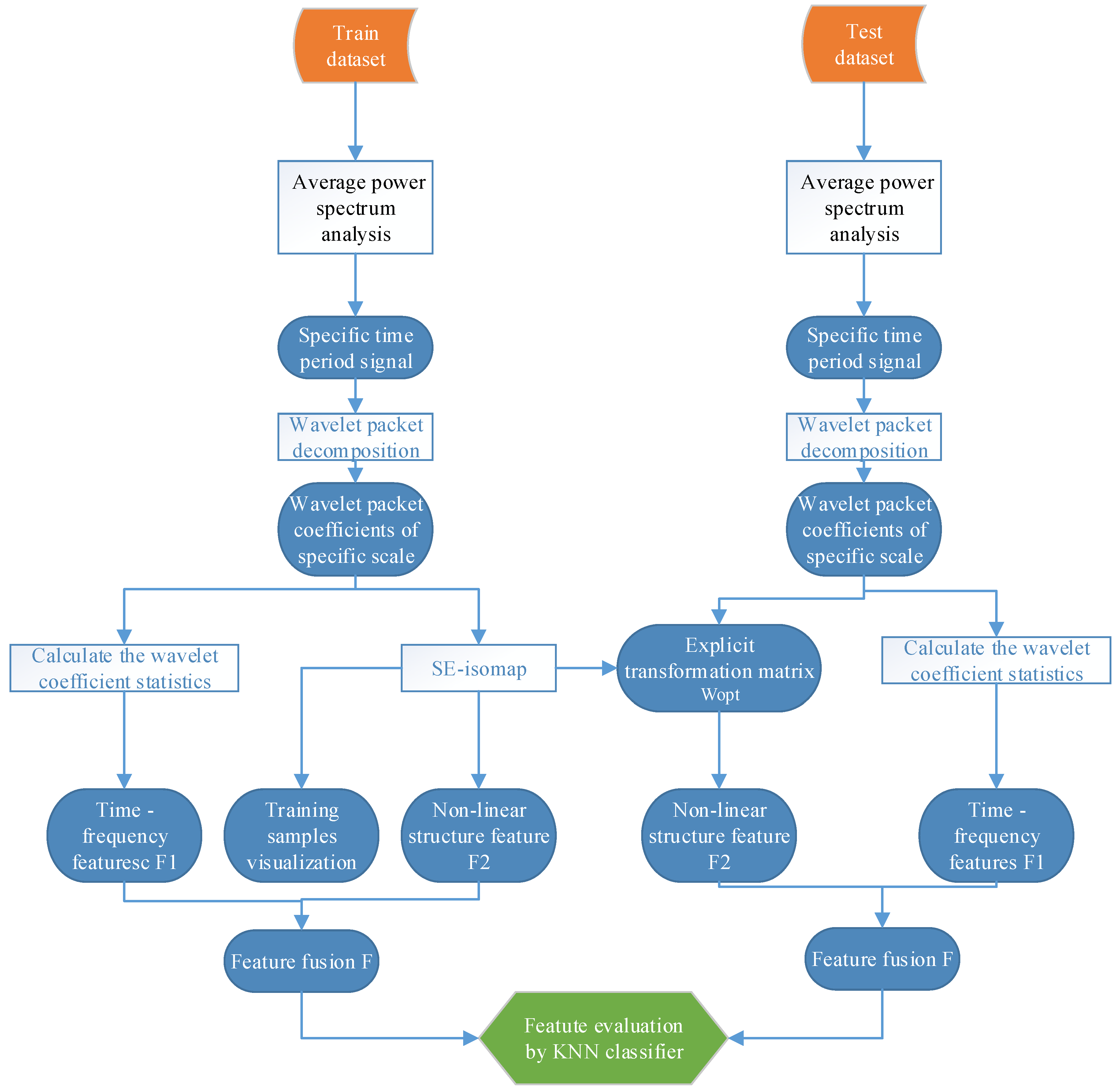
3. Feature Extraction Method Based on WPD and SE-Isomap

In this section, the feature extraction method is developed with WPD and SE-isomap, and it includes mainly three aspects: effective time segment selection, optimal wavelet packet selection and feature extraction and serial fusion. The flow chart of the proposed method is shown in Figure 2, in which the KNN classifier is used to evaluate the effectiveness of the MI-EEG features.

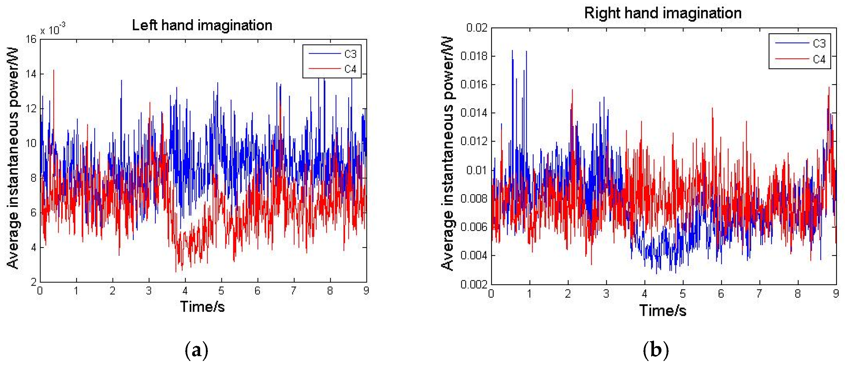
3.1. Instantaneous Power Spectra Analysis

In this study, the instantaneous power of each signal is calculated, and the instantaneous power of all signals is averaged to obtain the average instantaneous power spectrum of the signal. Suppose that dataset $\mathit{X}=\left[{\mathit{x}}_1,{\mathit{x}}_2,\dots ,{\mathit{x}}_i,\dots ,{\mathit{x}}_N\right]$, where N denotes the number of samples, ${\mathit{x}}_i={\left[x_i^1,x_i^2,\dots x_i^j,\dots ,x_i^D\right]}^{\mathrm{T}}$, $x_i^j$ is the j-th point of the i-th sample and D describes the original dimension of the samples. Then, the average power of the j-th point in the sample set can be calculated by:

$$P\left(j\right)=\frac{1}{N}{\displaystyle \sum }_{i=1}^N{(x_i^j)}^2$$

(14)

By comparing the average power spectrum over the entire time period, the most obvious time period of event-related synchronization (ERS)/event-related desynchronization (ERD) phenomenon [22] was determined, and the specific time interval was taken as the dataset for subsequent analysis.

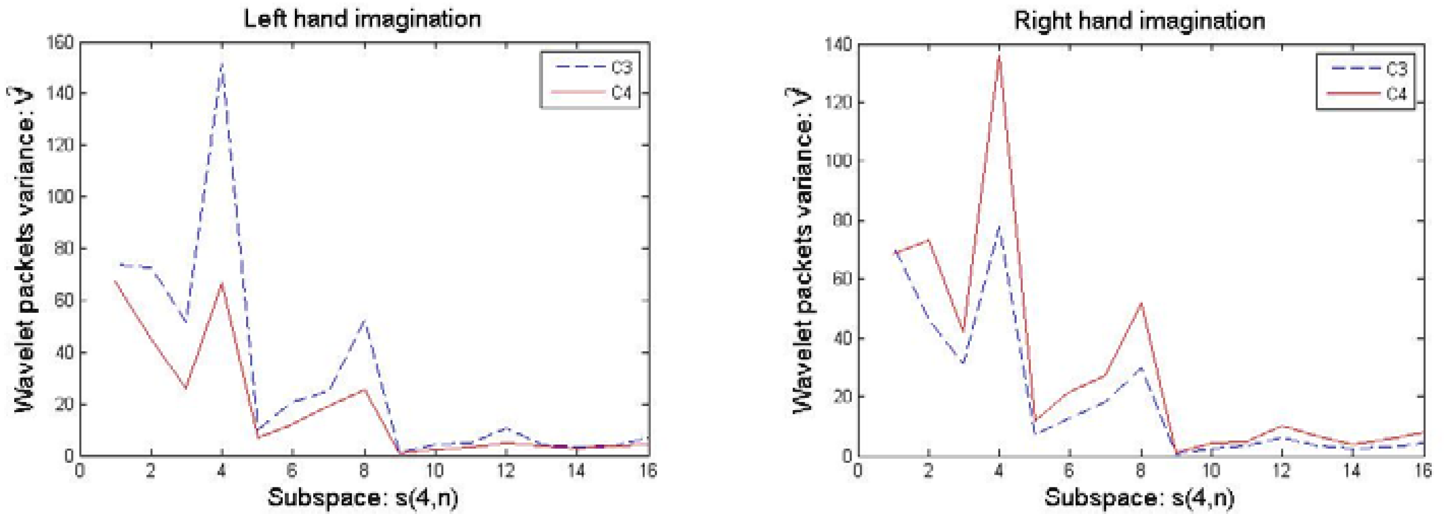
3.2. Selection of Optimal Wavelet Packets

The frequency bands and associated powers of the MI-EEG signal, which is collected through the brain and the cortical region related to motion, may change with different imaginary actions and different subjects. The recognition of MI-EEG is primarily based on the ERS/ERD-related motion-sensing rhythm characteristics. Therefore, the wavelet packet transform is the best choice to decompose the MI-EEG signal ${\mathit{x}}_i$ that is pre-determined by power spectra analysis, and wavelet packet variance is used to select the subject-based frequency bands or subject-specific wavelet packets. Suppose that the corresponding WPD coefficients to wavelet packet s(j,n) for the sample ${\mathit{x}}_i$ are denoted as $d_{l,j}^{n,i}\left(k\right)$, where l = 3 or 4; it is the label of channel C3 or C4; j is the number of decomposed levels; n is the number of wavelet packet subspaces in the j-th level; and k is the index of the coefficient sequence. According to the wavelet packet structure theory, if the wavelet basis function is orthogonal, the WPD will then comply with the energy conservation principle [21], that is the square sum of the WPD coefficients on each layer does not change when the number of decomposition layers changes. It can be formulated as:

$${\displaystyle \sum }_{n=0}^{2^j-1}{\displaystyle \sum }_{k=1}^K{\left|d_{l,j}^{n,i}\left(k\right)\right|}^2\equiv {\parallel f^2\parallel }^2$$

(15)

where K is the number of wavelet packet coefficients for subspace s(j,n) and ${\left|d_{l,j}^{n,i}\left(k\right)\right|}^2$ and ${\parallel f\parallel }^2$ represent the energy density and energy of the wavelet packet, respectively. The energy of n-th wavelet packet subspace is calculated as:

$$E_n={\displaystyle \sum }_{k=1}^K{\left|d_{l,j}^{n,i}\left(k\right)\right|}^2$$

(16)

The variance of the n-th WPS is defined as:

$$V_n^2={\sigma }_n^2=\frac{1}{K}{E}_n^2=\frac{1}{K}{\displaystyle \sum }_{k=1}^K{\left|d_{l,j}^{n,i}\left(k\right)\right|}^2$$

(17)

Then, the variance of different wavelet packets at a specific level is obtained.

After j-level WPD of the MI-EEG signal ${\mathit{x}}_i$, the WPD coefficients $d_{l,j}^{n,i}$ are divided into $2^j$ subspaces s(j,0) ~ s(j,$2^j-1$).

Then, according to Equation (17), the variance of the wavelet packet coefficients for each subspace under the specific layer j is calculated, and the wavelet packet variance of each subspace on this level is computed and added. The mean variance is obtained as follows:

$$\overline{V_n^2}=\frac{1}{N}{\displaystyle \sum }_{i=1}^N{\displaystyle \sum }_{k=1}^K{\left|d_{l,j}^{n,i}\left(k\right)\right|}^2$$

(18)

where $\overline{V_n^2}$ denotes the mean value of wavelet packet variance for all samples, N represents the number of samples and K is the dimension of wavelet packet coefficients.

For each motor imagery task, the j-level WPD of MI-EEG $x_i$ (i = 1, 2, …, N) on channels C3 and C4 is first completed. After that, the mean wavelet packet variances corresponding to channels C3 and C4 are calculated, respectively, for each wavelet packet s(j,n) ($n=0,1,\dots ,2^j-1$), and the difference between the mean wavelet packet variances is computed and sorted in the descending order. The partial wavelet packets referring to the top m mean variance difference are thought of as the OWP; this means they will have the most significant distinction for each motor imagery task. All of the OWP coefficients are constructed as a vector and denoted as:

$${\mathit{W}}_f^i={\left[d_{3,j}^{n_1,i}\left(1\right),\dots ,d_{3,j}^{n_1,i}\left(K\right),\dots ,d_{3,j}^{n_m,i}\left(1\right),\dots ,d_{3,j}^{n_m,i}\left(K\right),d_{4,j}^{n_1,i}\left(1\right),\dots ,d_{4,j}^{n_1,i}\left(K\right),\dots ,d_{4,j}^{n_m,i}\left(1\right),\dots ,d_{4,j}^{n_m,i}\left(K\right)\right]}^T\in R^{1\times \left(m\times K\times 2\right)},$$

where $n_1,n_2,\dots ,n_m$ are the indexes of the selected OWP subspaces.

3.3. Feature Extraction

3.3.1. Statistical Features Based on OWP

A series of WPD coefficients will be obtained after the MI-EEG signal is decomposed by WPD, and they carry the important time-frequency feature information. Here, the OWPs with the top q mean variance difference are found, and their coefficients are used in the calculation of statistical features. Let $d_{l,j}^{n,i}\left(k\right)$ be the decomposition coefficients of the s(j,n) subspace for the sample $x_i$ over channel Cl, then their statistics are defined as follows:

$${\overline{\mu }}_n^l=\frac{1}{K}{\displaystyle \sum }_{k=1}^K{d}_{l,j}^{n,i}\left(k\right)$$

(19)

$${\overline{E}}_n^l=\frac{1}{K}{\displaystyle \sum }_{k=1}^K{\left(d_{l,j}^{n,i}\left(k\right)\right)}^2$$

(20)

$${\overline{S}}_n^l=\sqrt{\frac{1}{K}{\displaystyle \sum }_{k=1}^K{\left(d_{l,j}^{n,i}\left(k\right)-{\overline{\mu }}_n^l\right)}^2}$$

(21)

where ${\overline{\mu }}_n^l$ represents the mean of the coefficients in the frequency band corresponding to the s(j,n) subspace and ${\overline{E}}_n^l$ and ${\overline{S}}_n^l$ denote the mean energy and mean standard deviation, respectively.

The ERS/ERD phenomenon can be expressed by C3 and C4 electrodes when the brain is implementing the imagination of left or right hand movement. To have the maximum separability for two motor imagery tasks, the time-frequency characteristics are defined as follows:

$$F_1=\left\{{\overline{\mu }}_{n_1}^3-{\overline{\mu }}_{n_1}^4,{\overline{E}}_{n_1}^3-{\overline{E}}_{n_1}^4,{\overline{S}}_{n_1}^3-{\overline{S}}_{n_1}^4,\dots ,{\overline{\mu }}_{n_q}^3-{\overline{\mu }}_{n_q}^4,{\overline{E}}_{n_q}^3-{\overline{E}}_{n_q}^4,{\overline{S}}_{n_q}^3-{\overline{S}}_{n_q}^4\right\}{R}^{1\times \left(3\times q\right)}$$

(22)

where $n_1,n_2,\dots ,n_q$ denote the indexes of the selected OWPs.

3.3.2. Non-Liner Structure Feature with SE-Isomap

Suppose that the OWP coefficient vectors ${\mathit{W}}_{\mathrm{f}}^i$(i = 1, 2, …, N) have been achieved from Section 3.2 for each class $C_b\left(b=1,2\right)$, which is really one of two motor imagery tasks. Then, the intra-class and inter-class geodesic distance between any two coefficient vectors are calculated according to Equations (3) and (4), and they are constructed as the matrices ${\mathit{G}}_{11}$, ${\mathit{G}}_{12}$ and ${\mathit{G}}_{22}$. Therefore, the global geodesic distance discriminant matrix $\mathit{G}=\left(\begin{array}{c}{\rho }_1{\mathit{G}}_{11}{\mathit{G}}_{12}\\ {\mathit{G}}_{21}{\rho }_2{\mathit{G}}_{22}\end{array}\right)$ can be obtained.

Next, the explicit MDS algorithm is applied to obtain the explicit mapping matrix ${\mathit{W}}_{\mathrm{opt}}$ by an iterative optimization algorithm and a low-dimensional representation of the training samples according to the global discriminant distance matrix G from the previous step. Then, the radial basis function $\mathit{\Phi }\left(x\right)$ of the test sample is obtained according to Equation (9). Finally, the low-dimensional representation of the test sample is obtained according to $\mathit{y}={\mathit{W}}_{\mathrm{opt}}^{\mathrm{T}}\mathit{\Phi }\left(x\right)$. The new nonlinear feature, representing the manifold structure, is denoted as ${\mathit{F}}_2=\left[y_1,y_2,\dots ,y_d\right]\in R^{1\times d}$, where d represents the feature dimension.

3.3.3. Feature Fusion

To take full advantage of the information obtained from multiple aspects, features ${\mathit{F}}_1$ and ${\mathit{F}}_2$ are integrated by using a serial connection, and they will be standardized before feature fusion to prevent the uneven weight caused by the difference of magnitude for two types of features. The equation is as follows:

$$\mathit{F}=\left[\frac{{\mathit{F}}_1}{\parallel {\mathit{F}}_1\parallel },\frac{{\mathit{F}}_2}{\parallel {\mathit{F}}_2\parallel }\right]\in R^{1\times （\left(3\times q\right)+d）}$$

(23)

where $\parallel ·\parallel$ denotes the two normal form.

3.4. Feature Evaluation

In the proposed extraction method, SE-isomap, as a nonlinear dimensionality reduction technology, is based mainly on the intrinsic geometry of the dataset; the extracted features contain the intrinsic geometry information of the data, and the geodesic distance between the features are the basis of the intrinsic geometry of the dataset. Therefore, the KNN algorithm with geodesic distance has the most direct and simple idea, and it will be the best choice for feature evaluation.

4. Experimental Research

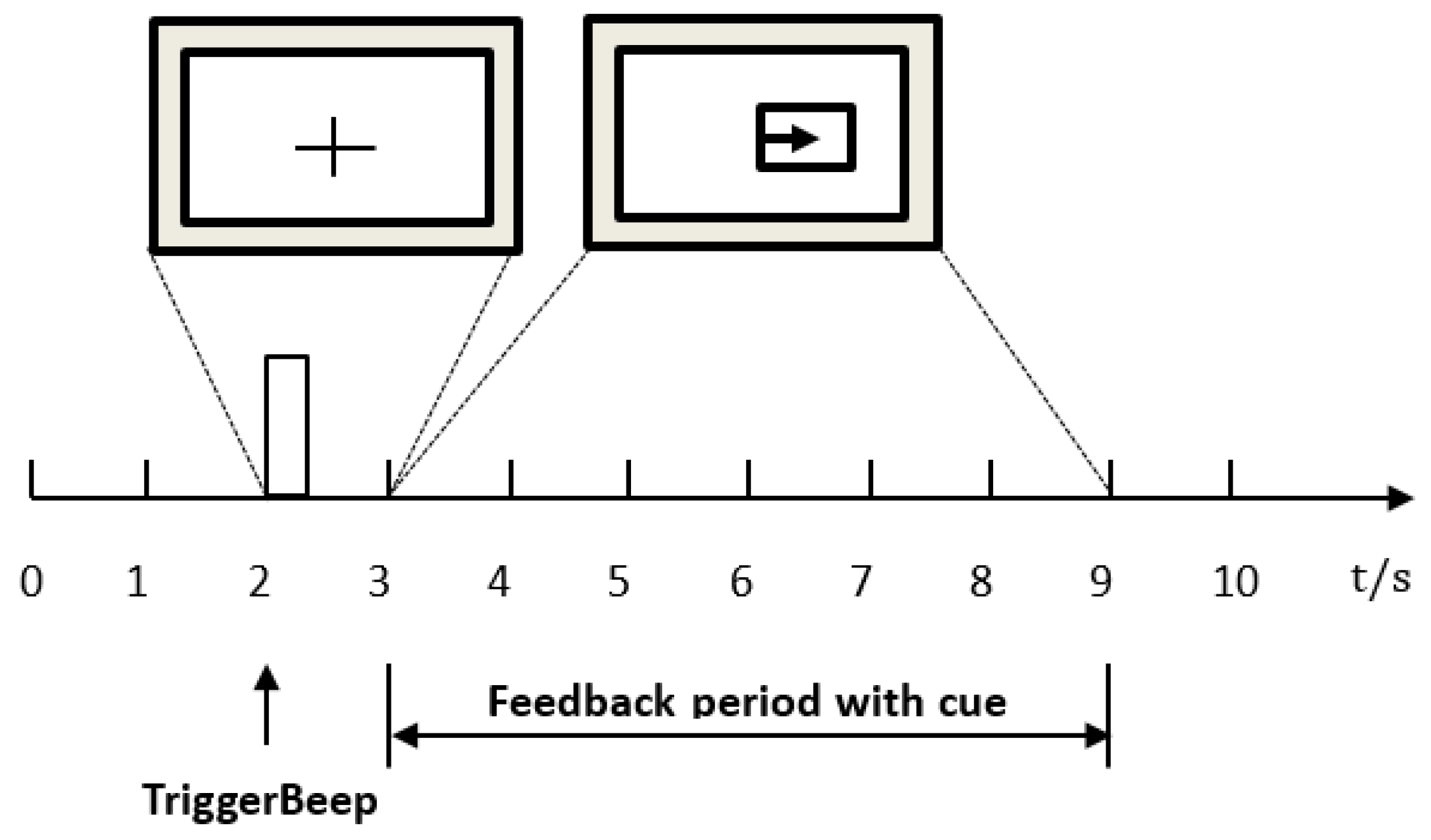
4.1. Dataset

The MI-EEG data in this study, published in BCI Competition 2003, are provided by BCI lab, Graz University of Technology. Signals were collected in a healthy adult female when imagining left and right hand movements. The dataset consists of 280 trials, in which 140 trials are left hand imagination and the rest are right hand imagination. The data are sampled at 128 Hz. Each trial lasts 9 s, and the sequence diagram of the experiment is shown in Figure 3. During the first 2 s, the subject keeps quiet and calm; when t = 2 s, a “+” cursor appears on the screen for 1 s, accompanied by a short beep indicating the start; at the third second, the “+” is replaced by the arrows indicating left or right direction as the direction of motor imagery.

4.2. Data Preprocessing and Determination of the Optimal Time Interval

The work in [22] showed that the ERS/ERD phenomenon in channels C3 and C4 is the most distinct when imagining the left and right hand movements. Therefore, to maximize the significant difference between ERD and ERS, the signals on channels C3 and C4 were selected in this study; channel Cz is discarded because of the lack of valid information related to the imaging task [26].

To determine the optimal time period related to the task and obtain the most distinguishable dataset, the average instantaneous power of MI-EEG over electrodes C3 and C4 under different imaging tasks was calculated, respectively, and this is shown in Figure 4.

It can be seen from Figure 4 that the average instantaneous power spectra of electrodes C3 and C4 show distinct ERS/ERD phenomena from 3.5 s to 6.5 s under different hand movement imagination tasks. Therefore, the time segment [3.5, 6.5] s is chosen as the optimal time period, on which the data are taken as the experimental sample in the follow-up study.

4.3. Time-Frequency Analysis with WPD

4.3.1. Selection of the Optimal Wavelet Packet Basis Function

WPD has been widely used in non-stationary signal processing. The multi-scale decomposition and time-frequency domain localization are implemented by using the scale and displacement operations, and the time-frequency resolution of a signal is effectively improved. Meanwhile, the specific time-frequency domain information is easily obtained [20]. It is noticeable that the analysis result is affected by the wavelet packet basis function [22], because the part of the signal whose wave form is similar to one of the selected basis function will be amplified. However, there are no reliable and effective methods to guide us to choose the basis function; therefore, the optimal wavelet packet basis function will be determined according to the classification effect through experiments. Here, several basis functions, including Symlets, Coiflets, Haar and Daubechies, which are similar to MI-EEG signal, are selected, and the proposed method is applied to extract the features of MI-EEG. The parameter setting is d = 16 and σ = 11 in SE-isomap, and the KNN classifier (parameter setting: k = 7) is adopted to identify the features and evaluate the suitability of basis functions. The average classification accuracy with 10-fold cross-validation is shown in

Table 1. Classification accuracy with different basis functions.

Basis Function	sym6	sym10	coif4	coif2	Haar	db4	db5
Accuracy (%)	81.7	82.4	87.2	88.3	90.1	92.7	89.8

.

As can be seen from Table 1, the classification result of the db4 basis function is significantly better than others; therefore, db4 is selected as the best wavelet basis function for the following research. In fact, among different types of basis functions, the Daubechies family is known for its orthogonality property and efficient filter implementation [27]. db4 was found to be the most appropriate basis for analysis of EEG data since the lower order wavelets of the family was too coarse to represent EEG spike properly, and the higher one cannot represent the spiky form of the EEG signal [28].

Additionally, the accuracy resulting from the Haar basis function also shows a comparable performance, and it is necessary to analyze the differences of the results between the Haar and db4 basic function statistically. In the following, a two-sample t-test is applied to identify whether there is a significant difference when they are used for MI-EEG feature extraction. Suppose that $M_{\mathrm{haar}}$ and $M_{\mathrm{db}4}$ stand for the mean value of the 10-fold cross-validation’s accuracies from the Haar and db4 basic function, respectively, $S_{\mathrm{haar}}^2$ and $S_{\mathrm{db}4}^2$ denote the variance, and $n_{\mathrm{haar}}$ and $n_{\mathrm{db}4}$ represent the number of the results. Then, the t-test statistic can be calculated as:

$$t=\frac{M_{\mathrm{db}4}-M_{\mathrm{haar}}}{\sqrt{\frac{\left(n_{\mathrm{db}4}-1\right)S_{\mathrm{db}4}^2+\left(n_{\mathrm{haar}}-1\right)S_{\mathrm{haar}}^2}{n_{\mathrm{db}4}+n_{\mathrm{haar}}-2}\left(\frac{1}{n_{\mathrm{db}4}}+\frac{1}{n_{\mathrm{haar}}}\right)}}$$

(24)

Assume that the null hypothesis is $H_0$: the results of Haar and db4 come from independent random samples from normal distributions with equal means; the alternative hypothesis is $H_1$: the results of Haar and db4 come from populations with unequal means. The significance level was chosen as $\alpha =0.05$. The decision rule is to reject $H_0$, if:

$$p=P\{t>t_{\alpha }\left(n_{\mathrm{haar}}+n_{\mathrm{db}4}-2\right)\}\le 0.05$$

(25)

After being calculated, the p-value is equal to 0.0131, which is less than 0.05; therefore, the null hypothesis is rejected at the 0.05 significance level. Hence, statistically, the performance of the db4 basic function significantly increases when compared with Haar.

4.3.2. Selection of Optimal Wavelet Packets

In this section, the four-level WPD is implemented for the MI-EEG sample on the time interval 3.5–6.5 s, and a series of WPD coefficients is obtained. Then, the mean variance of the wavelet packet coefficients is calculated for each subspace s(4,n) (n = 0, 1, …, 15) according to Equation (18). The results are shown in Figure 5.

It can be seen from Figure 5 that the difference of the wavelet packet variance is relatively obvious for the subspaces of s(4,1), s(4,2), s(4,3), s(4,5), s(4,6), s(4,7) and s(4,11), which are just the subject-specific optimal wavelet packets, and their corresponding sub-bands are 4–8 Hz, 8–12 Hz, 12–16 Hz, 20–24 Hz, 24–28 Hz, 28–32 Hz and 44–48 Hz, respectively.

4.3.3. Calculation of Time-Frequency Features

Based on the optimal wavelet packets and Equation (22), the time-frequency feature vector ${\mathit{F}}_1$ can be calculated in statistics, and the resulting classification accuracy can also be obtained. It is gratifying that the classification rate basically remains unchanged when the number of OWPs used for the computation of feature ${\mathit{F}}_1$ is more than three according to the experiments; therefore, q = 3, and${\mathit{F}}_1=\left\{{\overline{\mu }}_1^3-{\overline{\mu }}_1^4,{\overline{\mu }}_3^3-{\overline{\mu }}_3^4,{\overline{\mu }}_7^3-{\overline{\mu }}_7^4,{\overline{E}}_1^3-{\overline{E}}_1^4,{\overline{E}}_3^3-{\overline{E}}_3^4,{\overline{E}}_7^3-{\overline{E}}_7^4,{\overline{S}}_1^3-{\overline{S}}_1^4,{\overline{S}}_3^3-{\overline{S}}_3^4,{\overline{S}}_7^3-{\overline{S}}_7^4\right\}\in R^{1\times 9}.$

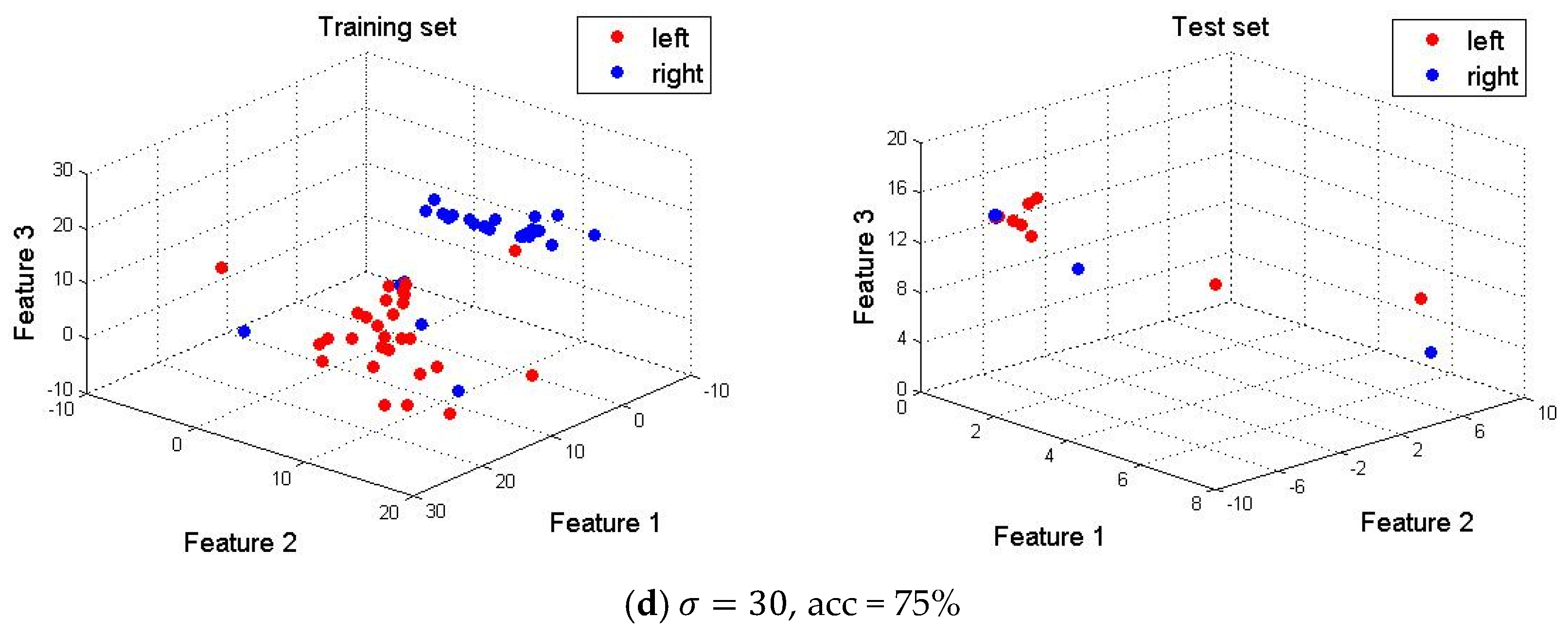
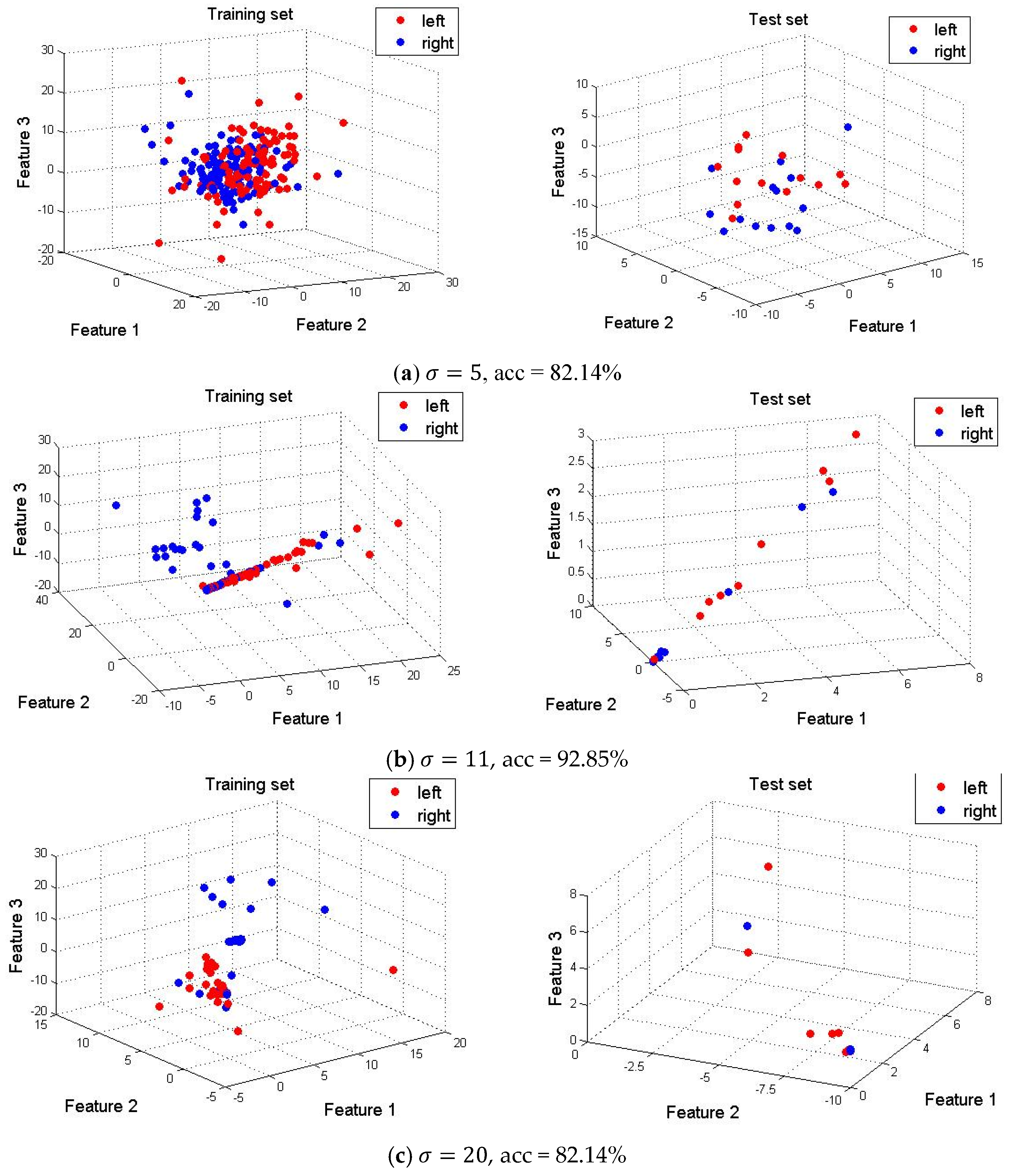
4.4. Dimension Reduction and Feature Visualization

On account of discovering the spatial structure information hidden in the MI-EEG, the SE-isomap algorithm is used to reduce the dimension of OWP coefficients. The inter-class distance σ and target spatial dimension d are two important parameters in SE-isomap. Under some different parameters σ, the proposed method is applied to dimension reduction for the training set and test set, respectively, and the most obvious three-dimensional features from the 16-dimension feature vector are visualized to discover the relationship and regularities between samples by a more intuitionistic way. Meanwhile, the accuracy of single experiment is provided to discuss the relationship between parameter $\sigma$ and the classification accuracy. The experiment results of visualization are as below. In Figure 6, acc represents the classification accuracy on the test dataset.

As shown in Figure 6, the features of training sample sets whose dimension is reduced by the SE-isomap algorithm show the clustering characteristics in a three-dimensional space, and with the increase of σ, the distance of the training datasets between different classes becomes larger at the same time. In Figure 6a, the aliasing still exists between the training samples. When the inter-class distance parameter σ increases, the separation of inter-class datasets is improved. It can be seen that the selection of parameter σ has a great influence on the feature visualization of EEG signals. It is clear from Figure 6b that the features of test samples show a linearly-separable distribution in the three-dimensional space. Although the visualization of the training samples is better when the inter-class distance parameter σ is larger, too large a value will bring a negative impact on the structure of the explicit mapping and also affect the true structural relationship between the data points, as shown in Figure 6c,d, which makes the distribution of the data points in the test set deviate significantly from their intrinsic geometry location, the overlapping phenomena occurring in a very small range due to the structural damage of some sample points, and ultimately leading to an unsatisfactory classification result. Therefore, it is very necessary to choose the value of σ reasonably for obtaining an ideal classification result.

4.5. Optimal Selection of Parameters in SE-Isomap

From Section 4.4, it can be seen that the feature visualization is affected by the inter-class distance parameter σ. In fact, the target spatial dimension d is another parameter impacting on the feature quality. To obtain the optimal values, the parameters are traversed in a reasonable range, and the optimal parameters are determined by the classification accuracy. The experiment results are shown in Figure 7.

As we can see from Figure 7, the classification accuracy changes with different parameters d and σ, and the best result is achieved when the parameters d = 16 and σ = 11. The optimal parameter values will remain in the subsequent experiments, and the nonlinear feature is easily obtained by ${\mathit{F}}_2=y\in R^{1\times 16}$.

4.6. Determination of Parameter k in the KNN Classifier

The KNN classifier is used to classify and evaluate the features in this research. However, the performance of the KNN classifier is influenced by the value of parameter k, and it is necessary to determine the optimal value of k through experiment. First, the geodesic distance from the feature points in the testing set to the ones in the training set is calculated, and the geodesic distance matrix G is obtained. Then, the matrix G is input in the KNN classifier together with the training sample label. Finally, the test sample label estimated by the KNN classifier is compared with the real label, and the classification result is shown in

Table 2. Comparison with different parameter k values.

k-Value	1	2	3	4	5	6	7	8	9
Accuracy (%)	82.9	83.1	86.2	87.5	88.3	90.6	92.7	89.1	91.2

.

It is clear that the classification accuracy reached the highest when k = 7. However, the result of k = 9 is close to that of k = 7. To ensure the rigor of the results, a two-sample t-test is applied to identify whether there is a significant difference of the results between k = 7 and k = 9, and the assumption is similar to the one in Section 4.3.1. The p-value is 0.0206, which is less than 0.05; therefore, the null hypothesis is rejected at the 0.05 significance level. Hence, statistically, the performance of k = 7 significantly increases when compared with k = 9. To guarantee the comparability, the parameter k = 7 will be kept constant in the next comparison experiments.

4.7. Comparison of Variety of Feature Extraction Algorithm Combined with WPD

To verify the validity of WPD combined with dimension reduction technology, this paper integrates the time-frequency features extracted by WPD with the nonlinear features extracted by different dimensionality reduction methods, and the new hybrid features are input in the KNN classifier. A series of classification results is shown in

Table 3. Comparison with other feature extraction methods (%). MDS, multidimensional scaling; LLE, locally linear embedding.

Methods	Feature Dimension	Accuracy	Methods	Feature Dimension	Accuracy
PCA	317	68.1 ± 6.3	WPD + PCA	96	73.1 ± 10.3
ICA	78	85.9 ± 8.9	WPD + ICA	42	87.3 ± 6.2
MDS	112	73.6 ± 7.4	WPD + MDS	84	77.4 ± 12.8
LLE	24	86.3 ± 4.2	WPD + LLE	33	91.8 ± 3.5
SE-isomap	16	88.5 ± 6.5	WPD + SE-isomap	25	92.7 ± 3.9

, in which the parameters for all feature extraction methods have been optimized, respectively.

It can be seen from Table 3 that when the WPD is combined with any one of the common dimension reduction algorithms, including PCA, ICA, MDS, LLE and SE-isomap, its classification result is superior to the corresponding dimension reduction algorithm alone. Additionally, the combination of WPD and SE-isomap, as a feature extraction method, yields the highest recognition accuracy and shows a good stability in this study. This also indicates the necessity and correctness of the combination of time-frequency information ${\mathit{F}}_1$ and of non-linear structure information ${\mathit{F}}_2$ in processing of the MI-EEG signal. In consideration of the results from the WPD + LLE and WPD + isomap methods being relatively close, a two-sample t-test, whose assumption is similar to the one in Section 4.3.1, was also implemented here to verify the statistical difference between the two feature extraction methods, and the p-value is 0.0497, which implies that the performance of WPD + isomap is significantly better than that of WPD + LLE.

4.8. Comparison of the Computational Cost with Multi-Feature Extraction Methods

The advantage of the SE-isomap algorithm is that both the low-dimensional representation of the data and the explicit mapping relationship of the data from the high-dimensional observation space to the low-dimensional representation space can be obtained at the same time, which facilitates the feature extraction of the new samples and improves the classification efficiency of the test sample. This is beneficial to the online realization of the recognition algorithm. Therefore, the training time and test time for multi-feature extraction methods, including PCA, MDS, etc., are recorded, respectively. The classification accuracies and their standard deviations are shown in

Table 4. Comparison of the computational cost.

Methods	Training Time (s)	Test Time (s)	Classification Rate (%)
PCA	152.2	1.7	68.1 ± 6.3
MDS	35.3	1.5	73.6 ± 7.4
LLE	207.2	2.7	86.3 ± 4.2
WPD	99.5	2.3	82.7 ± 8.8
SE-isomap	325.7	0.61	88.5 ± 6.5
WPD + PCA	258.7	7.9	73.1 ± 10.3
WPD + ICA	195.1	6.4	87.3 ± 6.2
WPD + MDS	140.5	4.3	77.4 ± 12.8
WPD + LLE	312.6	5.3	91.8 ± 3.5
WPD + SE-isomap	515.3	0.68	92.7 ± 3.9

. The experimental environment is the Windows 10 64-bit operating system; the CPU is Intel (R) Core (TM) i3 M370; the memory is 4 G; the software is MATLAB R2014a; and KNN is selected as the classifier in each experiment uniformly.

From Table 4, it can be seen that the SE-isomap method takes the longest time in the training procedure when WPD has not been implemented; however, the test time is the shortest. This is mainly resulting from the explicit mapping matrix. At the same time, the classification accuracy of SE-isomap is also the highest. As combined with WPD, the time consumption of WPD + SE-isomap in the training procedure is still the longest; however, the test time consumes slightly increases, and the classification accuracy increases from 88.5–92.7%. In addition, the classification accuracy of WPD + SE-isomap is the highest, and its standard deviation is nearly the lowest among all feature extraction methods. Hence, the proposed method is superior to other methods in terms of computational efficiency, classification accuracy and stability. It is verified that the explicit mapping matrix resulting from this method is helpful to reduce the computation cost, and extracted features are more complete and robust than that with other methods, showing the rationality of the combination of SE-isomap and WPD.

4.9. Comparison Study Based on a Multi-Subject MI-EEG Database

In order to verify the self-adaptive characteristic of the WPD + SE-isomap method, a comparison study is completed based on the BCI Competition 2008 Datasets 2b [29]. The database is composed of two classes, namely the motor imagery of left hand and right hand, and it consisted of the MI-EEG data from nine subjects. For each subject, five sessions are provided, whereby the first two sessions contain training data without feedback, and the last three sessions were recorded with feedback. Each session consisted of six runs with 10 trials per class and two classes of imagery. This resulted in 20 trials per run and 120 trials per person. In the following, a comparative experiment is conducted on the same training set and test set as [22]. The classification accuracies of two feature extraction methods for each subject are shown in

Table 5. Performance comparison of two feature extraction methods for 9 subjects (%). DFFS, dynamic frequency feature selection.

Subject	WPD + DFFS [22]	WPD + SE-Isomap
B01	73.24	84.58
B02	67.48	66.25
B03	63.01	62.92
B04	97.4	95.83
B05	95.49	89.17
B06	86.66	97.92
B07	84.68	82.08
B08	95.93	86.25
B09	92.61	97.08
Average	84.06	84.68

.

Table 5 indicates that the average recognition accuracy over nine subjects of WPD + SE-isomap has been improved slightly compared with WPD + DEFS [22]. Especially, the experiment results of the proposed method are better than WPD + DEFS for Subjects B01, B06 and B09, and they are as good as that of WPD + DEFS for Subjects B02, B03, B04 and B07. It is regretful that WPD + SE-isomap is not better than WPD + DEFS for Subjects B05 and B08. This is mainly because the proposed feature extraction needs sufficient training samples, and Sessions 1, 2 and 3 are provided as the training set only for Subjects B04, B06 and B09. It can be predicted that WPD + SE-isomap will show a clear advantage when the training set is adequate.

5. Conclusions

In this paper, an adaptive feature extraction method is proposed based on WPD and the SE-isomap algorithm for MI-EEG. The subject-specific optimal wavelet packets are selected; the associated wavelet packet coefficients are then used for the calculation of time-frequency statistical features and input in SE-isomap for the extraction of nonlinear manifold structure features. The hybrid features indicate the effectiveness in removing the redundant feature information and faithfully reconstructing the intrinsic structure for MI-EEG. Additionally, the explicit mapping relationship from the high-dimensional space to the low-dimensional space can be obtained by SE-isomap, and this is helpful for the reduction of the computational cost in feature extraction and the implementation of the on-line recognition algorithm. The extensive experiments are conducted on a public BCI dataset, and a relatively higher classification accuracy and smaller standard deviation are obtained simultaneously. In future work, the proposed method will be further improved to be suitable for more channels of the MI-EEG dataset and validated on more subjects. The technique of compressive sensing will be also taken into account to reduce the storage amount of MI-EEG [30].

References

- Wolpaw, J.R.; Birbaumer, N.; McFarland, D.J.; Pfurtscheller, G.; Vaughan, T.M. Brain–computer interfaces for communication and control. J. Clin. Neurophysiol. 2002, 113, 767–791. [Google Scholar] [CrossRef]
- Naseer, N.; Hong, K.S. Decoding answers to four-choice questions using functional near infrared spectroscopy. J. Infrared Spectrosc. 2015, 23, 23–31. [Google Scholar] [CrossRef]
- Hong, K.S.; Naseer, N.; Kim, Y.H. Classification of prefrontal and motor cortex signals for three-class fNIRS–BCI. Neurosci. Lett. 2015, 587, 87–92. [Google Scholar] [CrossRef] [PubMed]
- Naseer, N.; Hong, K.S. Classification of functional near-infrared spectroscopy signals corresponding to the right-and left-wrist motor imagery for development of a brain–computer interface. Neurosci. Lett. 2013, 553, 84–89. [Google Scholar] [CrossRef] [PubMed]
- Arvaneh, M.; Guan, C.; KengAng, K.; Quek, C. Optimizing spatial filters by minimizing within-class dissimilarities in electroencephalogram-based brain–computer interface. IEEE Trans. Neural Netw. Learn. Syst. 2013, 24, 610–619. [Google Scholar] [CrossRef] [PubMed]
- Liu, G.; Zhang, D.; Meng, J.; Huang, G.; Zhu, X. Unsupervised adaptation of electroencephalogram signal processing based on fuzzy C-means algorithm. Int. J. Adapt. Control Signal Process. 2012, 26, 482–495. [Google Scholar] [CrossRef]
- Millan, J.R. On the need for on-line learning in brain–computer interfaces. In Proceedings of the 2004 IEEE International Joint Conference on Neural Networks, Budapest, Hungary, 25–29 July 2004; pp. 2877–2882. [Google Scholar]
- Yu, X.; Chum, P.; Sim, K.B. Analysis the effect of PCA for feature reduction in non-stationary EEG based motor imagery of BCI system. Optik 2014, 125, 1498–1502. [Google Scholar] [CrossRef]
- Geng, X.; Zhan, D.C.; Zhou, Z.H. Supervised nonlinear dimensionality reduction for visualization and classification. IEEE Trans. Syst. Man Cybern. B Cybern. 2005, 35, 1098–1107. [Google Scholar] [CrossRef] [PubMed]
- Krivov, E.; Belyaev, M. Dimensionality reduction with isomap algorithm for EEG covariance matrices. In Proceedings of the 2016 4th International Winter Conference on Brain-Computer Interface (BCI), Yongpyong, Korea, 22–24 February 2016. [Google Scholar]
- Amin, H.U.; Malik, A.S.; Ahmad, R.F.; Badruddin, N.; Kamel, N.; Hussain, M.; Chooi, W.-T. Feature extraction and classification for EEG signals using wavelet transform and machine learning techniques. J. Australas. Phys. Eng. Sci. Med. 2015, 38, 139–149. [Google Scholar] [CrossRef] [PubMed]
- Tenenbaum, J.B.; Silva, V.; Langford, J.C. A Global Geometric Framework for Nonlinear Dimensionality Reduction. Science 2000, 290, 2319–2323. [Google Scholar] [CrossRef] [PubMed]
- Roweis, T.; Saul, K. Nonlinear dimensionality reduction by locally linear embedding. Science 2000, 29, 2323–2326. [Google Scholar] [CrossRef] [PubMed]
- Li, C.G.; Guo, J.; Chen, G.; Nie, X.F.; Yang, Z. A version of isomap with explicit mapping. In Proceedings of the Fifth International Conference on Machine Learning and Cybernetics, Dalian, China, 13–16 August 2006. [Google Scholar]
- Sadatnejad, K.; Ghidary, S.S. Kernel learning over the manifold of symmetric positive definite matrices for dimensionality reduction in a BCI application. J. Neurocomput. 2016, 179, 152–160. [Google Scholar] [CrossRef]
- Mirsadeghi, M.; Behnam, H.; Shalbaf, R.; Moghadam, H. Characterizing awake and anesthetized states using a dimensionality reduction method. J. Med. Syst. 2016, 40, 13–21. [Google Scholar] [CrossRef] [PubMed]
- Li, C.G.; Guo, J. Supervised isomap with explicit mapping. In Proceedings of the First International Conference on Innovative Computing, Information and Control (ICICIC’2006), Beijing, China, 30 August–1 September 2006. [Google Scholar]
- Li, M.; Luo, X.; Yang, J. Extracting the nonlinear features of motor imagery EEG using parametric t-SNE. J. Neurocomput. 2016, 218, 371–381. [Google Scholar] [CrossRef]
- Yang, B.; Li, H.; Wang, Q.; Zhang, Y. Subject-based feature extraction by using fisher WPD-CSP in brain–computer interfaces. Comput. Methods Programs Biomed. 2016, 129, 21–28. [Google Scholar] [CrossRef] [PubMed]
- Wu, T.; Yan, G.Z.; Yang, B.H.; Sun, H. EEG feature extraction based on wavelet packet decomposition for brain computer interface. Measurement 2008, 41, 618–625. [Google Scholar]
- Kevric, J.; Subasi, A. Comparison of signal decomposition methods in classification of EEG signals for motor-imagery BCI system. J. Biomed. Signal Process. Control 2017, 31, 398–406. [Google Scholar] [CrossRef]
- Luo, J.; Feng, Z.; Zhang, J.; Lu, N. Dynamic frequency feature selection based approach for classification of motor imageries. J. Comput. Biol. Med. 2016, 75, 45–53. [Google Scholar] [CrossRef] [PubMed]
- Boonnak, N.; Kamonsantiroj, S. Wavelet Transform Enhancement for Drowsiness Classification in EEG Records Using Energy Coefficient Distribution and Neural Network. Int. J. Mach. Learn. Comput. 2015, 5, 288–293. [Google Scholar] [CrossRef]
- Yan, S.; Zhao, H.; Liu, C.; Wang, H. Brain-Computer Interface Design Based on Wavelet Packet Transform and SVM. In Proceedings of the 2012 International Conference on Systems and Informatics (ICSAI 2012), Yantai, China, 19–20 May 2012. [Google Scholar]
- Xu, B.G. Feature extraction and classification of single trial motor imagery EEG. J. Southeast Univ. 2007, 37, 629–633. [Google Scholar]
- Pfurtscheller, G.; Da Silva, F.H.L. Event-related EEG/MEG synchronization and desynchronization: Basic principles. J. Clin. Neurophysiol. 1999, 110, 1842–1857. [Google Scholar] [CrossRef]
- Hu, D.; Li, W.; Chen, X. Feature extraction of motor imagery EEG signals based on wavelet packet decomposition. In Proceedings of the IEEE/ICME International Conference on Complex Medical Engineering (CME), Harbin, China, 22–25 May 2011; pp. 694–697. [Google Scholar]
- Adeli, H.; Zhou, Z.; Dadmehr, N. Analysis of EEG records in an epileptic patient using wavelet transform. J. Neurosci. Methods 2003, 123, 69–87. [Google Scholar] [CrossRef]
- Leeb, R.; Brunner, C.; Müller-Putz, G.; Schlögl, A.; Pfurtscheller, G. BCI Competition 2008—Graz Data Set B; Graz University of Technology: Graz, Austria, 2008. [Google Scholar]
- Morabito, F.; Labate, D.; Bramanti, A.; La Foresta, F.; Morabito, G.; Palamara, I.; Szu, H.H. Enhanced compressibility of EEG signal in Alzheimer’s disease patients. IEEE Sens. J. 2013, 13, 3255–3262. [Google Scholar] [CrossRef]