Hierarchical Wavelet-Aided Neural Intelligent Identification of Structural Damage in Noisy Conditions

Abstract

A sophisticated hierarchical neural network model for intelligent assessment of structural damage is constructed by the synergetic action of auto-associative neural networks (AANNs) and Levenberg-Marquardt neural networks (LMNNs). With the model, AANNs aided by the wavelet packet transform are firstly employed to extract damage features from measured dynamic responses and LMNNs are then utilized to undertake damage pattern recognition. The synergetic functions endow the model with a unique mechanism of intelligent damage identification in structures. The model is applied for the identification of damage in a three-span continuous bridge, with particular emphasis on noise interference. The results show that the AANNs can produce a low-dimensional space of damage features, from which LMNNs can recognize both the location and the severity of structural damage with great accuracy and strong robustness against noise. The proposed model holds promise for developing viable intelligent damage identification technology for actual engineering structures.

1. Introduction

Structural damage identification has been an active research focus that has been receiving increased attention over the years in the civil engineering field. Structural accidents have once again demonstrated the necessity of developing valid techniques for early-stage structural damage identification [1,2]. In general, structural damage identification can be divided into four progressive levels: judgment of damage occurrence, determination of damage location, discrimination of damage severity, and assessment of remaining structural life [3,4]. Typical damage identification methods found in the literature are usually developed by processing structural dynamic responses. Such methods can be largely categorized into two groups: vibration-based damage detection methods [5,6,7] and wave-propagation-based damage inspection methods [8,9,10].

An active branch of vibration-based damage identification is damage pattern recognition based on artificial intelligence methods [11,12,13,14,15]. The most popular artificial intelligence method used in structural damage diagnosis is artificial neural networks (ANNs), providing the advantages of self-adaptiveness, generalization, and real-time processing [16,17,18]. Representative studies of ANN-based damage pattern recognition are described as follows. Worden et al. [19,20] applied ANNs to evaluate the location and severity of damage in monotonic structures. Ni et al. [21] proposed an ANN-based method using measured modal properties to detect damage in steel frames, testifying to the effectiveness of discriminating positions and degrees of multiple instances of damage. Zubaydi et al. [22] used ANNs to interrogate damage in the side shells of a ship structure, illustrating the capacity of ANNs to discover such damage. Sahoo et al. [23] proposed a hybrid neuro-genetic algorithm to automate the design of a neural network for different types of structures. The neural network was trained considering frequency and strain as the input parameters, location and the amount of damage as the output parameters. Its performance was demonstrated using two test problems and the results were quite encouraging. Hakim and Razak [24] summarized the existing studies of using measured frequent response functions (FRFs) as inputs to ANNs for structural damage identification, with the conclusion that FRFs held fair advantages over modal parameters in damage characterization.

In recent years, the wavelet signal processing technique, referring to the wavelet transform (WT) [25,26,27,28] and the wavelet packet transform (WPT) [29,30,31,32,33,34,35], has been incorporated into ANN-based damage pattern recognition, and that technique has become an active research focus of vibration-based structural damage identification. In this aspect, representative studies are as follows. Yam et al. [36] developed a method integrating ANNs and WT to locate and quantify damage in polyvinyl chloride sandwich plates, with satisfactory results obtained. Zhu et al. [37] integrated a wavelet real-time filtering algorithm, adaptive neuro-fuzzy inference system (ANFIS), and an interval modeling technique to process structural response signals and excitation data. The method they proposed could rapidly identify unknown damage and small damage. Diao et al. [38] combined WPT and ANNs to establish a two-step damage detection method that could locate and quantify damage with great robustness. Tara et al. [39] proposed a synergetic approach of damage detection by linking ANNs and WT, in which the wavelet energy was used as a damage feature to discriminate different damage patterns. Yan et al. [40] used probabilistic neural networks aided by the WPT to detect structural damage under ambient vibration. Evagorou et al. [41] extracted features from the moments of the probability density functions of the wavelet coefficients obtained through WPT, and then developed a classification algorithm on the basis of a probabilistic neural network. Torres et al. [42] preprocessed the acoustic-ultrasonic responses using the discrete WT to produce wavelet coefficients. The produced wavelet coefficients are then processed by the AANN for outlier analysis-based damage detection in pipeworks, with the damage detected accurately. In general, studies have emphasized the advances of ANNs in recognizing different damage patterns, aside from stating the capability of WT or WPT in extracting damage features.

Despite the prevalence of using ANNs for structural damage identification, a notable imperfection is that ANNs commonly take on the sole function of damage pattern recognition [43,44,45], they have barely played any role in extracting damage features to date. Owing to the flexibility and versatility, ANN techniques have marked potential for creating damage features. This potential can be of important significance in expanding the capacity of ANNs to be used in the field of structural damage identification. To this effect, this study presents an innovative hierarchical wavelet-aided neural intelligent diagnosis model that can achieve the functions not only of damage pattern recognition but also of damage feature extraction.

2. Fundamental Theories

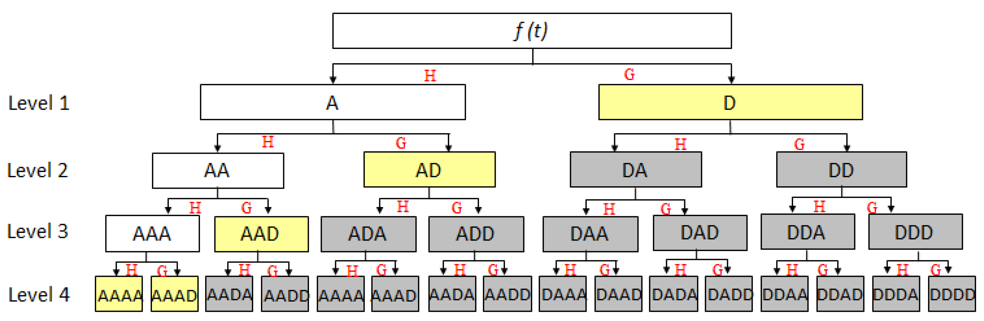
2.1. Wavelet Packet Transform (WPT)

The WPT is defined by the expressions [46,47]:

$$\{\begin{array}{c}{u}_{2n}^{(j)}(t)=\sqrt{2}{\displaystyle {\sum }_{k}h(k)u_n^{(j)}(2t-k)}\\ u_{2n+1}^{(j)}(t)=\sqrt{2}{\displaystyle {\sum }_{k}g(k)u_n^{(j)}(2t-k)}\end{array};n,k=0,1,2,\cdots$$

(1)

where $u_0^{(0)}(t)=\phi (t)$ is the scaling function, $u_1^{(0)}(t)=\psi (t)$ is the wavelet function, $j$ is the decomposition level, $k$ is the translation parameter, and $n$ is the modulation parameter. The terms $h(k)$ and $g(k)$ are quadrature mirror filters, and the corresponding function sets $H={\left\{h(k)\right\}}_{k=z}$ and $G={\left\{g(k)\right\}}_{k=z}$ denote the low pass filter and the high pass filter, respectively. The recursive relations between the $j\mathrm{th}$ and the $(j+1)\mathrm{th}$ level components of WPT are given in the equations:

$$f_j^i(t)=f_{j+1}^{2i-1}(t)+f_{j+1}^{2i}(t)$$

(2)

$$f_{j+1}^{2i-1}(t)=H{f}_j^i(t)$$

(3)

$$f_{j+1}^{2i}(t)=G{f}_j^i(t)$$

(4)

After being decomposed for $j$ times, the sum of the component signals can represent the original signal $f(t)$ as:

$$f(t)={\displaystyle \sum _{i=1}^{2^j}{f}_j^i(t)}$$

(5)

The process of WPT for the original signal can be perceived as a binary tree (Figure 1), in which $f(t)$ is at the top layer. At the first decomposition layer, $f(t)$ is decomposed by the filters H and G, giving its approximate component signal A and detail component signal D. A and D are then decomposed by H and G again, respectively, leading to two new pairs of approximate and detail component signals, {AA, AD} and {DA, DD}. For the next layer, the filters H and G are used in the same way to process each component signal AA, AD, DA, and DD, creating new pairs of approximate and detail component signals, and so on. In the end, at the $j\mathrm{th}$ layer, a total of $2^j$ component signals can be produced. All the component signals generated by the WPT up to the fourth layer are displayed in Figure 1, in which each component signal is termed a wavelet packet node.

In Figure 1, the upper-left part is the WT procedure; the component signals with yellow backgrounds D, AD, AAD, AAAD and AAAA are just the results of the WT. Hence, the WT is a subset of the WPT. Unlike the WT that merely covers the lower frequency part, the WPT provides even more and exhaustive decomposition along the whole frequency scope, because each left detail signal is decomposed again in a similar way to decompose the approximation signal. The down sampling operation of WPT causes the switch of the order of the low and high-pass components in a subsequent decomposition, hence producing a frequency content that follows a Gray code sequence [47].

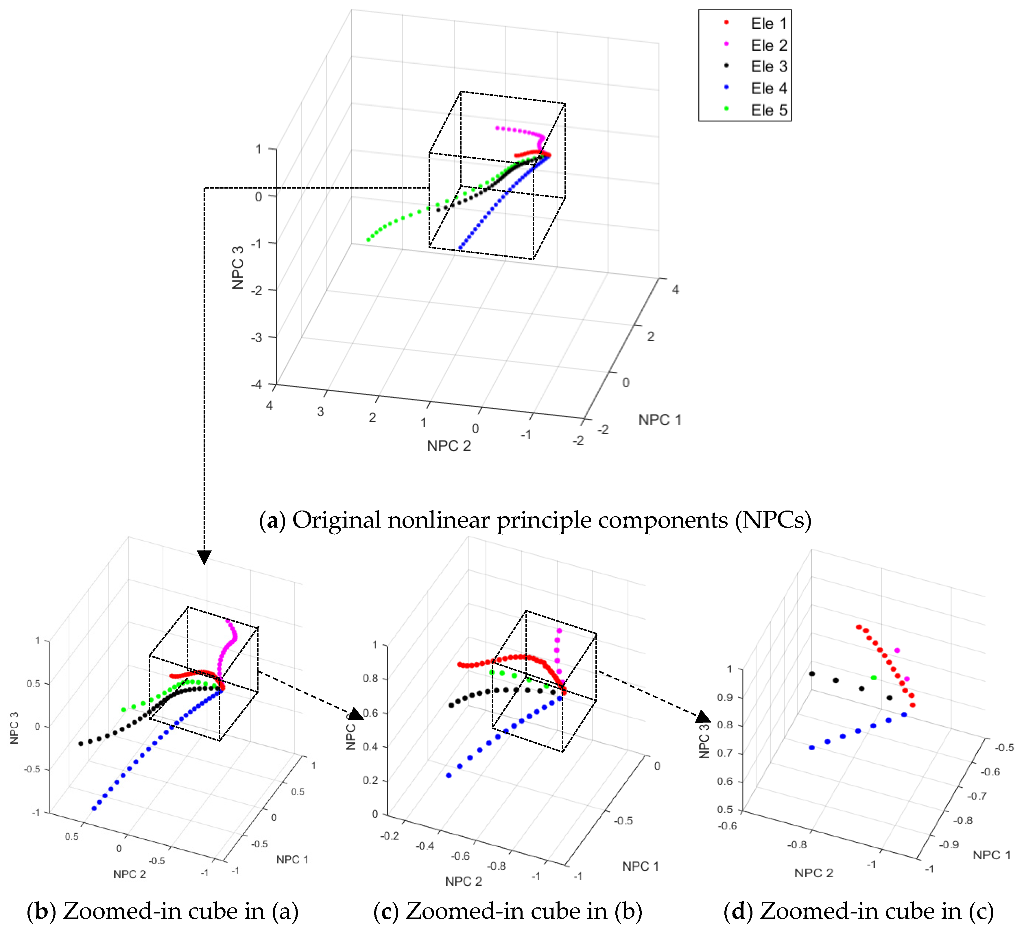
2.2. Nonlinear Principal Component Analysis

Nonlinear principal component analysis (NLPCA) is deemed to be a nonlinear generalization of principal component analysis (PCA) [48], generally used for data compression and dimension reduction, and can be realized by the following procedure.

Let $X$ be an original data set of high dimension. $X$ is projected by a nonlinear function vector $U$ into a new data set $T$ of low dimension:

$$T=U(X)$$

(6)

$T$ can be projected back into the original space by another nonlinear function vector $V$, giving $\widehat{X}$

$$\widehat{X}=V(T)$$

(7)

$\widehat{X}$ is the reconstruction of $X$ with the residual error $\tilde{X}$

$$\tilde{X}=X-\widehat{X}$$

(8)

The functions $U$ and $V$ are properly chosen to minimize the residual error. With appropriate $U$ and $V$, Equations (6) and (7) can be used to project a high-dimensional data set $X$ to a low-dimensional data set $T$ with little information loss, which is the essence of NLPCA.

Compared to the PCA, the NLPCA has two distinctive features: (i) it has advantages over the standard PCA in removing not only linear but also nonlinear correlations in variables; (ii) the nonlinear principal components (NPCs) from NLPCA are parallel in importance rather than being in decreasing order like those of the PCA.

Recent studies have reported that ANNs can implement some component analysis methods such as sensitivity analysis [49]. Likewise, they can be used to conduct NLPCA. Auto-associative neural networks (AANNs) have been demonstrated as a sophisticated strategy to carry out NLPCA [50]. The technological key lies in constructing an auto-associative learning framework by placing the high-dimensional data set $X$ at both the input and target output layers. As shown in Figure 2, AANNs consist of five layers: the input layer, the mapping layer, the bottleneck layer (low-dimensional space), the remapping layer, and the output layer. After being well trained by controlling the resident error defined by Equation (8), AANNs perform Equation (6) by projecting $X$ of high dimension from the input layer to $T$ of low dimension in the bottleneck layer via the mapping layer; meanwhile, AANNs perform Equation (7) by projecting $T$ from the bottleneck layer to $\widehat{X}$ in the output layer via the remapping layer.

Alternatively, AANNs can be seen as a combination of two individual networks, NN1 and NN2, with symmetrical structures. NN1 consists of the input layer, the mapping layer, and the bottleneck layer, whereas NN2 consists of the bottleneck layer, the remapping layer, and the output layer. The two networks integrate by sharing the bottleneck layer. It has been illustrated that for a neural network, one hidden layer with a nonlinear activation function is sufficient for modeling arbitrary nonlinear functions, so both NN1 and NN2 are able to model a nonlinear function if their activation functions in the hidden layer are nonlinear [50]. To ensure that the AANNs are capable for NLPCA, they should have nonlinear activation functions for the mapping and remapping layers.

3. Damage Identification Paradigm

A hierarchical neural intelligent model for structural damage identification is established by integrating the function of AANNs for extracting damage features with that of the LMNNs for recognizing damage patterns.

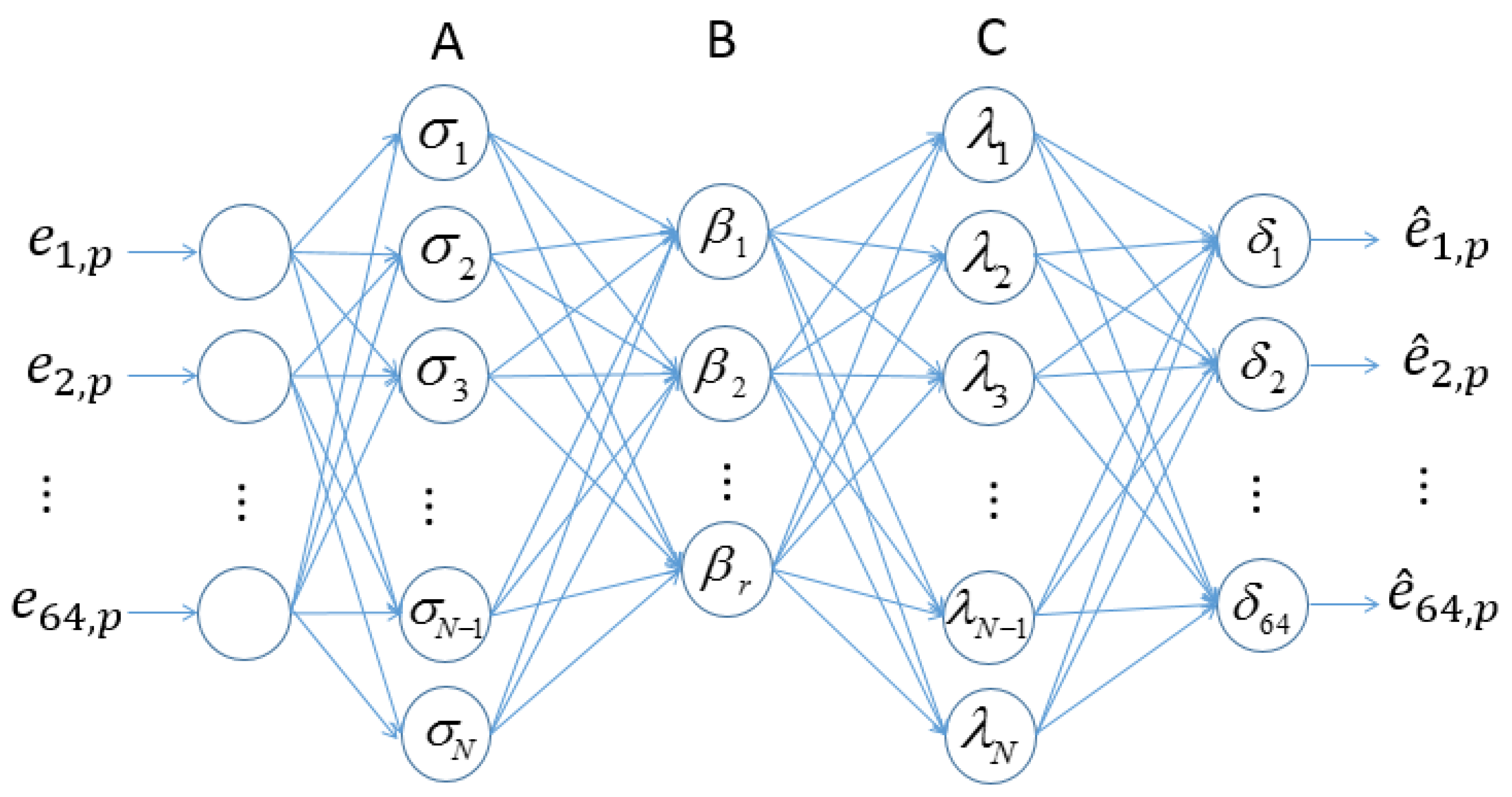
3.1. Formation of Damage Features Using AANNs

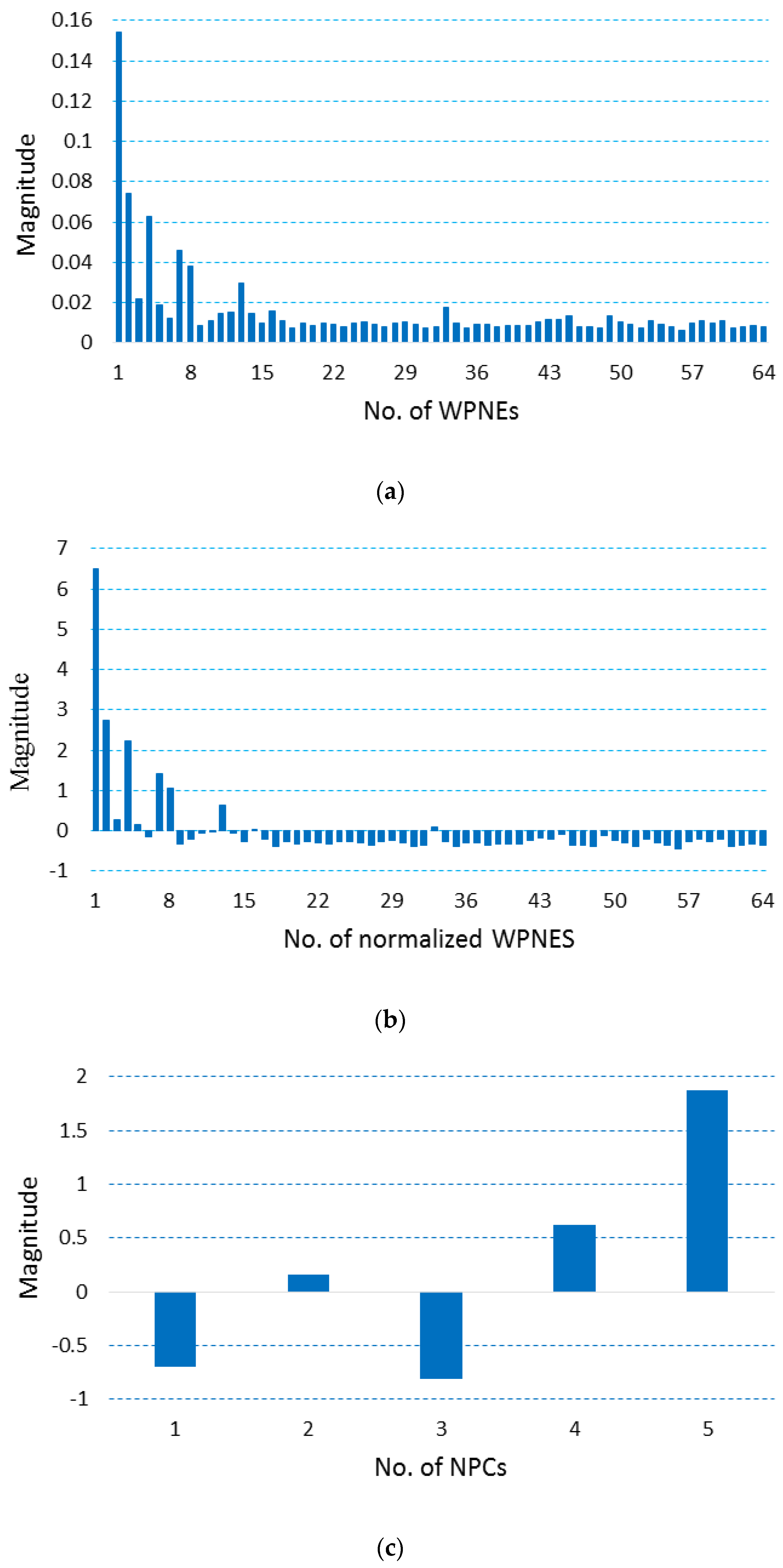
3.1.1. Wavelet Packet Node Energies (WPNEs)

The WPNEs of structural dynamic responses are newly emerging damage indices used in intelligent damage identification methods in recent studies [29,51]. Let $f(t)$ be an acceleration response of a structure subjected to an excitation. The WPNEs can be defined on $f(t)$ as:

$$E(i,j)={{\displaystyle {\sum }_k\left|d_j^i\left[k\right]\right|}}^2$$

(9)

$$d_j^i\left[k\right]=\langle f,u_{j,k}^n(t)\rangle ={\displaystyle \int f(t)u_{j,k}^n(t)}$$

(10)

where $i$ labels the $i\mathrm{th}$ wavelet packet node at the $j\mathrm{th}$ layer, $d_j^i\left[k\right]$ is the WPT coefficient of the $i\mathrm{th}$ wavelet packet node, $k$ is the translation parameter, and $u_{j,k}^n(t)$is the wavelet packet function. The principle of using WPNEs to represent damage is that damage can modulate the structural dynamic response, and therefore it can change the WPNE distribution derived from the dynamic response. Compared to traditional dynamic features such as frequency or modal shape, WPNEs are much more sensitive to damage. Moreover, WPNEs are more robust than some newer damage features such as the WPT coefficient. In what follows, WPNEs are used to characterize damage.

The operation of WPNEs in characterizing damage are related to the wavelet packet function and the decomposition level of the WPT. In this study, the wavelet packet function is set at Daubechies4 (db4) and the number of decomposition layers is set at six. The choice of the db4 wavelet as the mother wavelet in the WPT to decompose the acceleration for damage identification is based on the trial-and-error method. The trial-and-error method is a general method for determining the proper mother wavelet for use in the WT-based structural damage detection, typically referring to [42,51]. Equations (9) and (10) give rise to the vector of WPNEs, $e_p={\left(e_{1,p},e_{2,p},\cdots e_{64,p}\right)}^T$. Although this vector carries sufficient damage information, its high dimensionality causes considerable difficulty in the efficient representation of damage. In particular, it is unfeasible to employ the vector of WPNEs as damage features to frame an intelligent damage pattern recognition paradigm. This instance entails a procedure of extracting damage features from WPNEs. The extracted damage features should have the characteristic of low dimensionality and also preserve the damage information of the WPNEs.

3.1.2. Damage Feature Extraction

NLPCA was previously introduced in the field of structural damage detection, where it was mainly used to deal with environmental effects [52,53]. In this article, it helps build damage features. Considering that the WPNEs vector $e_p$ is a column vector, a matrix $E$ is constructed from the WPNEs vectors $e_p$ of $m$ samples as follows:

$$E=\left[\begin{array}{ccc}\begin{array}{cccc}{e}_{1,1}& e_{1,2}& \cdots & e_{1,p}\\ e_{2,1}& e_{2,2}& \cdots & e_{2,p}\\ ⋮& ⋮& \ddots & ⋮\\ e_{64,1}& e_{64,2}& \cdots & e_{64,p}\end{array}& \begin{array}{c}\cdots \\ \cdots \\ \ddots \\ \cdots \end{array}& \begin{array}{c}{e}_{1,m}\\ e_{2,m}\\ ⋮\\ e_{64,m}\end{array}\end{array}\right]=\left(\begin{array}{ccc}\begin{array}{ccc}\begin{array}{cc}{e}_1& e_2\end{array}& \cdots & e_p\end{array}& \cdots & e_m\end{array}\right)$$

(11)

Extraction of damage features from WPNEs is tackled by the NLPCA strategy that is implemented by the AANNs, with the structure depicted in Figure 2. The number of neurons at the input layer or output layer (M) fits the dimensions of the WPNEs. According to [49], the number of neurons of either the mapping layer or the remapping layer N should be chosen such that:

2N < M

(12)

The bottleneck layer will produce NPCs that represent the extracted damage features. Therefore, the number of NPCs (r) equals the number of neurons in the bottleneck layer. r is properly chosen to ensure that the extracted damage features contain the sufficient damage information stored in the WPNEs. The activation functions in the mapping and remapping layers are the sigmoid functions $\sigma$ and $\lambda$, respectively, whereas the activation functions at the bottleneck and output layers are the pure line functions $\beta$ and $\delta$, respectively, as indicated in the circle of the corresponding layer in Figure 2. The cost function, measured by the mean squared error (MSE), directs the training of the AANNs, with the MSE defined by [50]:

$$MSE={\displaystyle \sum _{p=1}^m{\displaystyle \sum _{i=1}^{64}{\left(e_{i,p}-{\widehat{e}}_{i,p}\right)}^2}}$$

(13)

where $m$ is the number of samples. $e_{i,p}$ and ${\widehat{e}}_{i,p}$ are the target values and prediction values of the AANNs, respectively.

When the inputs and the target output are both set to WPNEs, the AANNs are forced to build a mapping from the inputs to the outputs. This mapping can produce a converted low-dimensional vector of WPNEs, i.e., the NPCs of WPNEs. In a well-trained AANN, the matrix of NPCs $C_{r\times m}$ with $r\ll 64$ is generated from the bottleneck layer. The $C$ matrix is formed:

$$C=\left[\begin{array}{ccc}\begin{array}{cccc}{c}_{1,1}& c_{1,2}& \cdots & c_{1,p}\\ c_{2,1}& c_{2,2}& \cdots & c_{2,p}\\ ⋮& ⋮& \ddots & ⋮\\ c_{r,1}& c_{r,2}& \cdots & c_{r,p}\end{array}& \begin{array}{c}\cdots \\ \cdots \\ \ddots \\ \cdots \end{array}& \begin{array}{c}{c}_{1,m}\\ c_{2,m}\\ ⋮\\ c_{r,m}\end{array}\end{array}\right]=\left(\begin{array}{ccc}\begin{array}{ccc}\begin{array}{cc}{c}_1& c_2\end{array}& \cdots & c_p\end{array}& \cdots & c_m\end{array}\right)$$

(14)

where $c_p$ is a vector of NPCs for a damage sample. The NPCs carry almost all the damage information of WPNEs but have lower dimensionality than the WPNEs. This peculiarity enables NPCs to be valid damage features for intelligent damage pattern recognition.

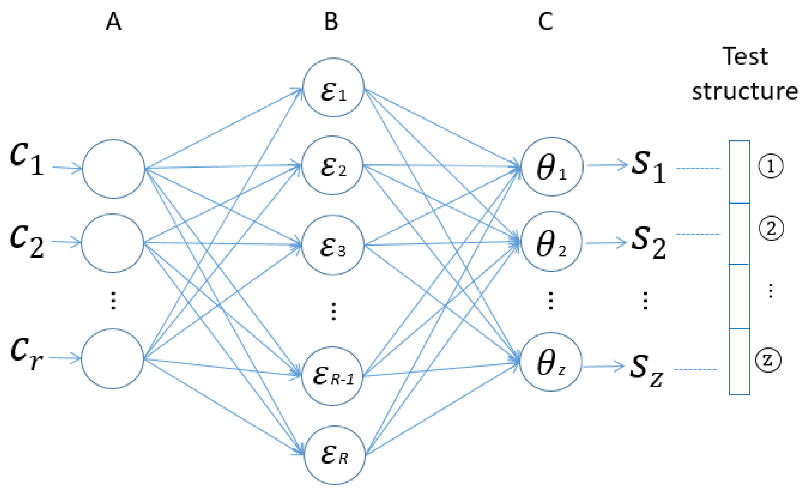
3.2. Damage Pattern Recognition

With the damage features extracted by AANNs as inputs, LMNNs are utilized to perform damage pattern recognition. The LMNNs are back-feed forward neural networks equipped with the Levenberg-Marquardt algorithm. This algorithm endows LMNNs with distinctive efficiency and precision in convergence [54]. As shown in Figure 3, the LMNNs consist of three layers: an input layer, a hidden layer, and an output layer. The Greek letters in the neuron circles represent activation functions of the corresponding layer. In the hidden layer, the activation function $\epsilon$ is the sigmoid function and in the output layer, $\theta$ is the pure line function. The inputs are the NPCs constructed from the AANNs, $C_{r\times m}$ with $r\ll 64$; the outputs $S_{z\times m}$ describe the spatial element distribution of the structure being inspected (Figure 3). The value of each entry from 0 to $a$ denotes the extent of the damage, with $a$ denoting the upper limit of the severity of possible damage. The spatial position of this entry in $S_{z\times m}$ indicates the damaged element of the structure.

To train the LMNNs, a certain number of damaged cases of the test structure need to be considered to construct the training sample set. Furthermore, more different damaged cases are demanded as testing samples for the network, to test its generalization ability after being well trained. For the particular model proposed here, due to the validity of the choices of inputs, relatively fewer training samples can train the LMNNs adequately. During the course of training, the LMNNs try to find out the underlying relationship between damage features (inputs) and damage states (outputs) by constantly adjusting the weight and bias of the hidden layer and output layer. MSEs between the outputs and the targets are considered as the cost function of the LMNNs. After being well trained, the LMNNs can build nonlinear mapping between damage features and damage states. This mapping will be able to recognize new unknown structural damage states.

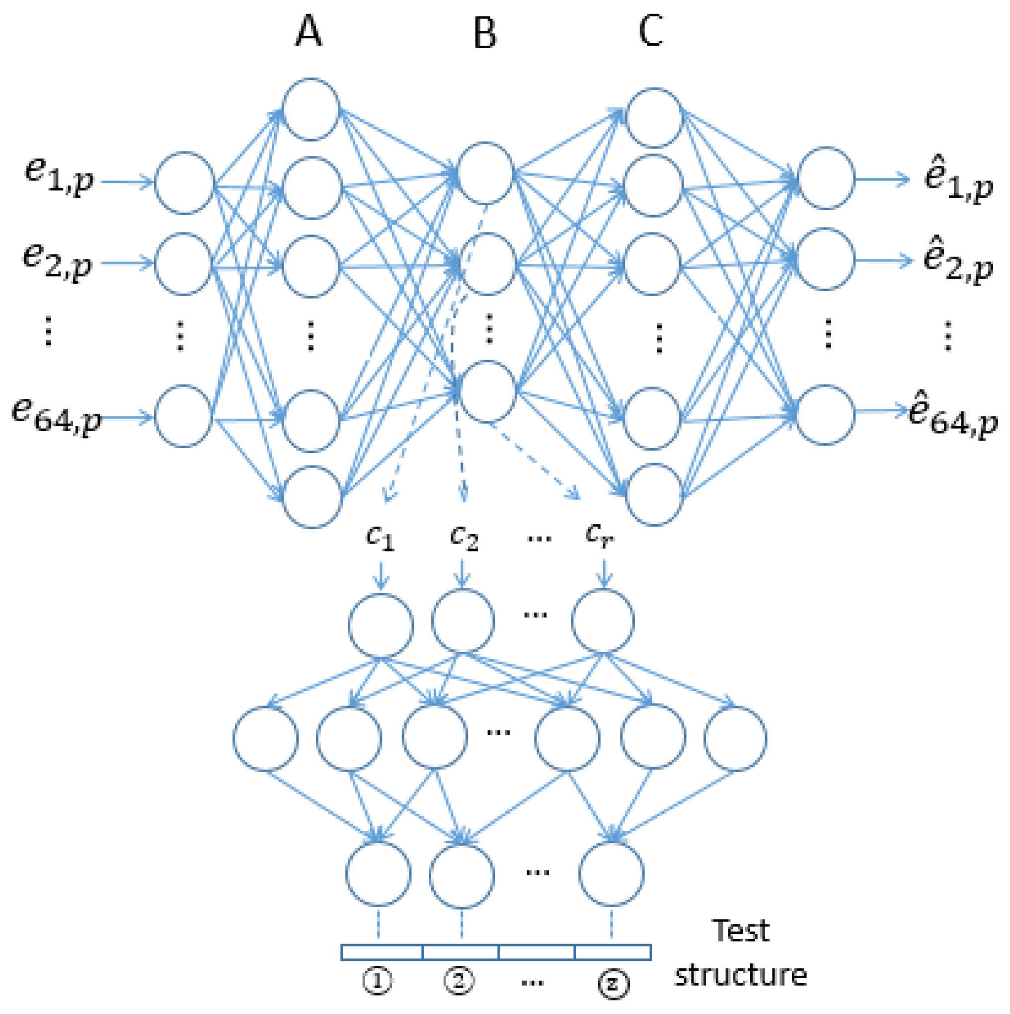
3.3. Hierarchical Neural Network Model

The synergetic action of AANNs and LMNNs constructs a hierarchical neural network model for intelligent damage assessment, as shown in Figure 4. In the process of damage identification, AANNs are responsible for damage feature extraction and LMNNs account for damage pattern recognition. Distinctive features of the proposed model in damage assessment are:

(i)

WPNEs are much more sensitive to damage than WPT coefficients, natural frequencies, and mode shapes.

(ii)

AANNs acting as a smart NLPCA tool can extract damage features from WPNEs. Such extracted damage features have lower dimensionality than WPNEs while preserving enough damage information.

(iii)

LMNNs can capture the underlying relations between damage features and damage states, on which they can recognize structural damage patterns.

(iv)

The special structure of the hierarchical neural network model requires a small set of training samples of damaged cases to produce accurate prediction results of damage identification with great noise robustness.

(v)

The hierarchical neural network model is easily implemented in a computational language, e.g., Matlab, to create an automatic program of intelligent damage assessment.

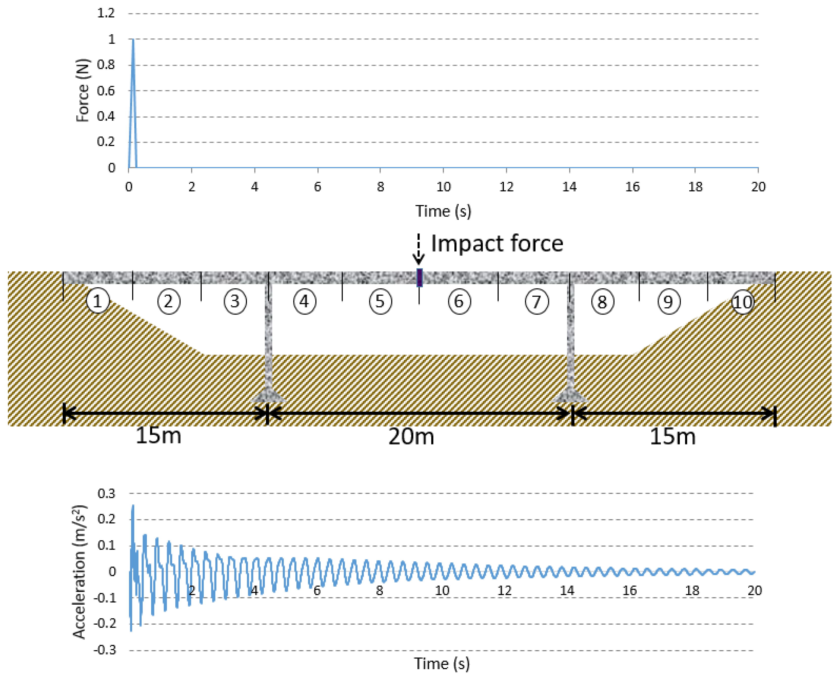
4. Numerical Verification

The three-span continuous bridge is a typical item in civil infrastructure. The effectiveness of the proposed model is verified by detecting damage in a three-span continuous bridge (Figure 5) with span lengths 15, 20, and 15 m, respectively, similar to the engineering case used in [55]. The material properties of the bridge are listed in

Table 1. Material properties of the bridge.

Properties	Values
Mass density	$7800$ ${\mathrm{kg}/\mathrm{m}}^2$
Young’s modulus	$200$ ${\mathrm{GN}/\mathrm{m}}^2$
Cross-sectional area	$5\times {10}^{-2}$ ${\mathrm{m}}^2$
Moment of inertial	$4.17\times {10}^{-6}$ ${\mathrm{m}}^2$
Damping ratio	$0.01$

and this bridge is modeled using ten beam elements. An impact force with a maximum magnitude of 100 N is exerted at the midpoint of the bridge, and the acceleration response of this point is measured. A duration of 20 s of acceleration response is recorded, with the sampling frequency of 100 Hz. From the acceleration response, the traditional modal properties including natural frequencies and mode shapes are first analyzed for damage characterization. Unfortunately, in the cases of damage with the stiffness reduction ratio (SRR) below 10%, the maximum change in the traditional parameters induced by the damage is less than 5%, insufficient to reflect the damage. This example, illustrating the incapacity of traditional modal characteristics to portray damage, calls for a more sophisticated method to undertake damage identification of the bridge.

4.1. Damage Cases

Damage is fabricated by reducing the stiffness of a finite element of the bridge. Damage severity is described by the SRR. For each element, a set of 30 damaged cases is elaborated with SRRs ranging from 1% to 30% (

Table 2. Layout of damage cases.

Case Number	Damaged Element	SRR (%)
1–30	1	1, 2, …, 30
31–60	2	1, 2, …, 30
61–90	3	1, 2, …, 30
91–120	4	1, 2, …, 30
121–150	5	1, 2, …, 30

). In total, 150 damaged cases are created in which damage occurs independently in one element of half of the bridge with various severities, considering the structure’s symmetry. For each damaged case, an impact force is exerted to vibrate the bridge, with the acceleration responses measured at the midpoint of the bridge.

4.2. Damage Feature Extraction

For preprocessing, the WPT is employed to process the acceleration responses and generate WPNEs. Let $f_p(t)$ be the acceleration response generated from the $p\mathrm{th}$ damaged case. The db4 wavelet optimally selected is used to decompose $f_p(t)$ up to the sixth layer, resulting in 64 WPNEs. Figure 6a,b show the WPNEs and their normalized forms of the intact case, where the normalization is conducted as:

$$e_{i,p}=\frac{\left(e_{i,p}-\overline{e}\right)}{\sigma }$$

(15)

where $\overline{e}$ and $\sigma$ are the mean value and the standard deviation of the WPNE vector.

In accordance with the procedure described in Section 3.2, the AANNs are employed to extract damage features from the WPNEs. By the trial-and-error method, the optimal number of neurons in the bottleneck layer of the AANNs is determined as 5; by the rule stated in Equation (12), the number of neurons in the mapping layer as well as the remapping layer is given as 20. When the WPNEs are individually placed in the input layer and the output layer, the AANNs can be driven to train under the control of the cost function, i.e., MSE. Once the AANNs are well trained, as indicated by the MSE arriving at the stop criterion, the outputs of the bottleneck layer generate the NPCs, leading to five NPCs. These NPCs are the damage features extracted from the WPNEs, as illustrated in Figure 6c for the intact case.

The damaged cases listed in Table 2 can be divided into five groups in terms of the damaged elements (locations), from Ele 1 to Ele 5, with Ele being an abbreviation of element. Damaged cases in same group differ from each other according to their different damage severities. Visualization of the NPCs is utilized to indicate their feasibility to characterize damage. The first three NPCs of all damage cases are plotted in Figure 7a, with Figure 7b–d providing progressively zoomed-in displays of the portion covered by the zoomed-in window. In these figures, there are five dotted curves extending to different directions, each comprising a sequence of separated dots. Each curve denotes a group of damage cases with the damage located at the same element; each dot of a curve labels a damage case of specific damage severity. The dispersion of the dotted curves indicates the effectiveness of the NPCs to reflect different damage locations; the separation of the dots in one curve designates the efficiency of the NPCs to characterize different damage severities. Clearly, the NPCs can be used to characterize not only the damage location but also the damage severity, even in damaged cases with the SRR less than 5%.

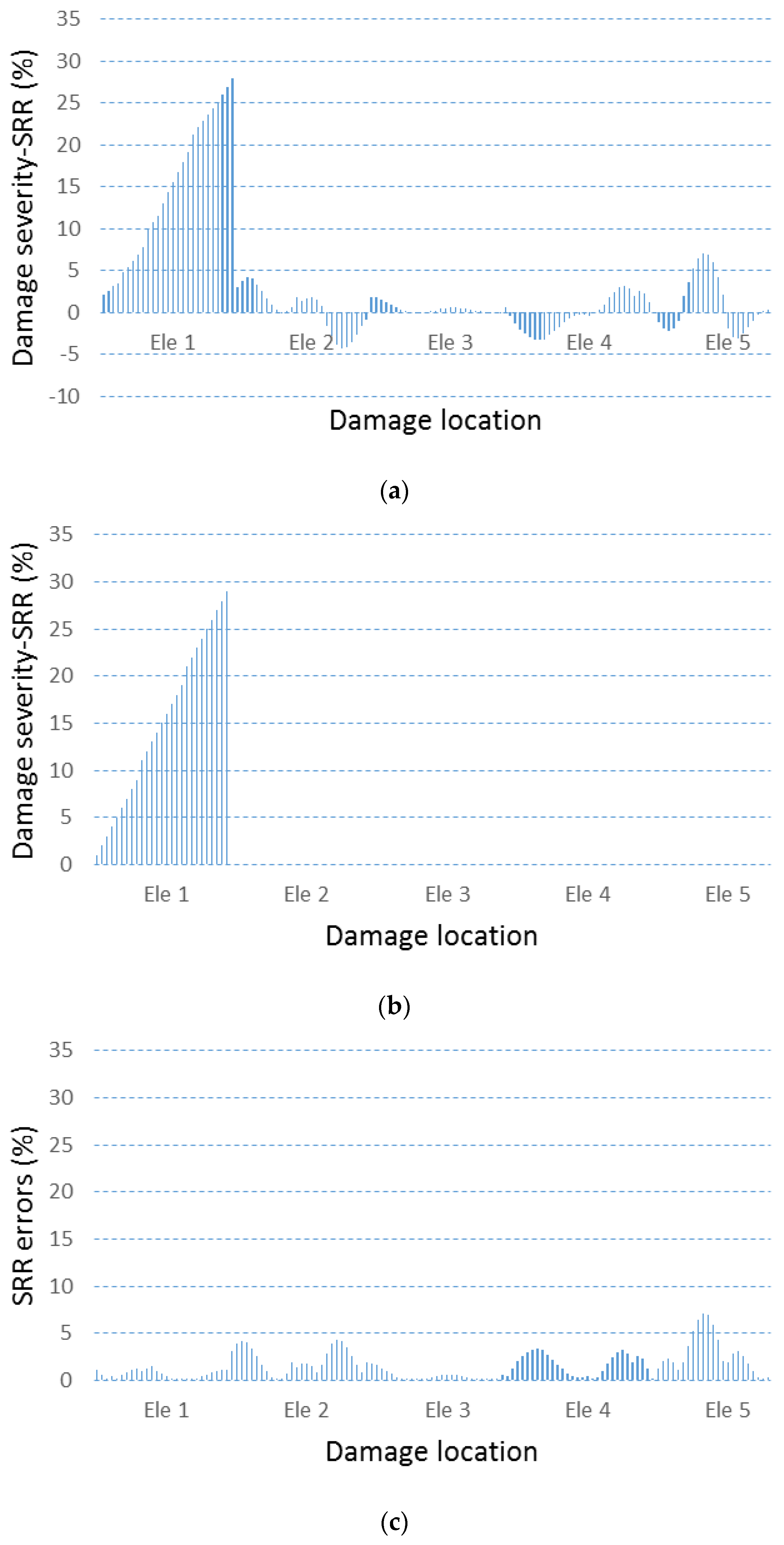
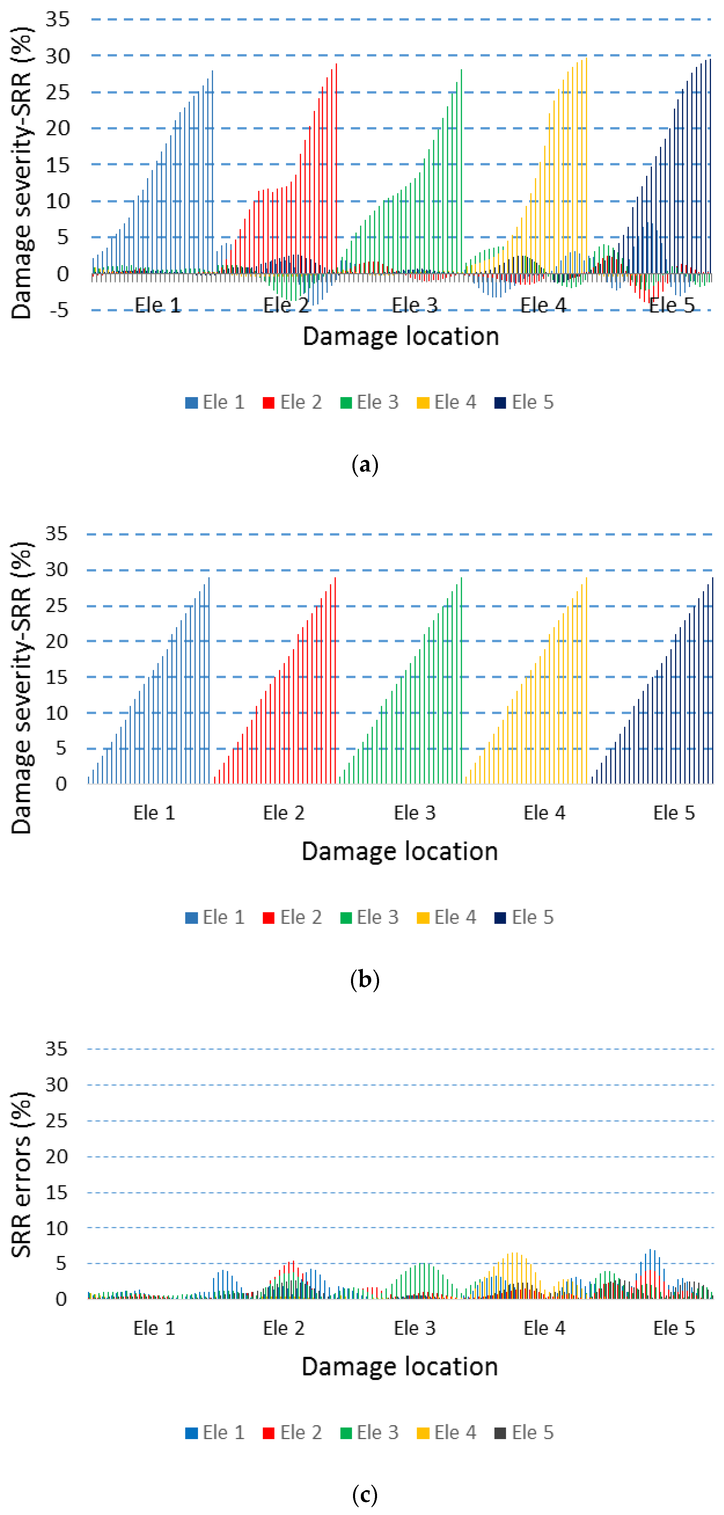
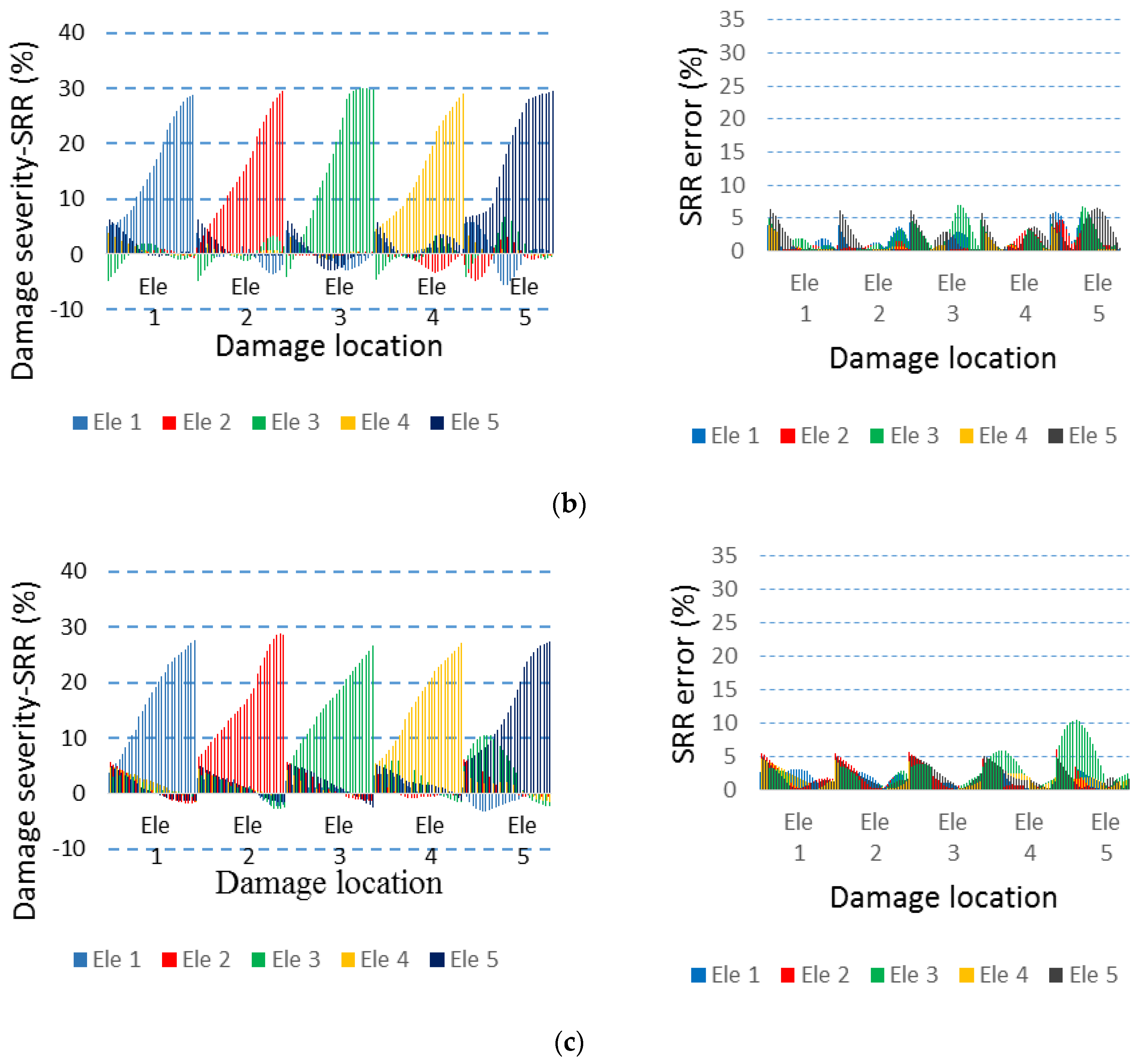
4.3. Damage Pattern Recognition

Following damage feature extraction using the AANNs, the LMNNs are used to recognize the damage location and severity. The inputs of LMNNs are the extracted damage features as illustrated in Figure 6c, and the outputs are five dimensional vectors [S_{Ele 1}, S_{Ele 2}, S_{Ele 3}, S_{Ele 4}, S_{Ele 5}], among which S_{Ele k} denotes the SRR of the $k\mathrm{th}$ element of the bridge. S_{Ele k} takes the value of the interval [0, 0.3], suggesting that the maximum severity of damage considered is SRR = 30%. When the SRR varies from 1% to 30% for each element, 150 damaged cases are elaborated, as listed in

Table 3. Training and testing set of samples for damage identification.

Element	Training Set	Testing Set
	SRR (%)	SRR (%)
1	10	1, 2, …, 9
	20	11, 12, …, 19
	30	21, 22, …, 29
2	10	1, 2, …, 9
	20	11, 12, …, 19
	30	21, 22, …, 29
3	10	1, 2, …, 9
	20	11, 12, …, 19
	30	21, 22, …, 29
4	10	1, 2, …, 9
	20	11, 12,…, 19
	30	21, 22, …, 29
5	10	1, 2, …, 9
	20	11, 12, …, 19
	30	21, 22, …, 29

Note: the intact bridge (SRR = 0) is a case of the training set.

. These damaged cases and the intact case are divided into a training set and a testing set of samples. The training set consists of 16 cases including 15 damaged cases that the SRR = 10%, 20%, 30% for each element and the intact case; the testing set comprises 135 damaged cases with SRRs differing from those in the training set. The training sample set is used to train the LMNNs with the cost function of MSE to control the training.

The LMNNs are considered well trained when the MSE reaches the stop criterion of $2\times {10}^{-5}$. This criterion is determined by a trial-and-error method to ensure enough accuracy (avoiding excessive training) and high efficiency. At this stage, fed with the damage feature vectors of the test samples, the LMNNs produce the estimated vectors of [S_{Ele 1}, S_{Ele 2}, S_{Ele 3}, S_{Ele 4}, S_{Ele 5}] for every sample. The difference between the estimated vectors and the target output vectors indicates the error of the damage identification. For instance, for the result corresponding to Ele 1, Figure 8a presents the output of Ele 1 estimated by the LMNNs for all the test samples; Figure 8b presents the associated target outputs; Figure 8c depicts the difference between the estimated values and the target outputs, i.e., the damage identification error. Clearly, the Ele 1 output of the LMNN approximates the target very well. For all the test samples, the damage identification results are given in Figure 9a–c for the estimated values, targets outputs, as well as the identification error. Firstly, the damage location can be detected with great accuracy; there are few incorrect judgments of the damage location. For the aspect of damage severity, some errors obstruct from obtaining a very precise prediction of the severity of damage. However, those errors are within a small range. As seen in Figure 9c, the errors are all below an upper limit of about seven, indicating that the detection may only fail for some minor damage. In a word, the results show that the proposed hierarchical neural network model can effectively detect both the location and severity of damage.

Notably, the proposed model has considerable generalization capability; it can capture the underlying relations between damage features and damage states on the basis of a fairly limited number of training samples.

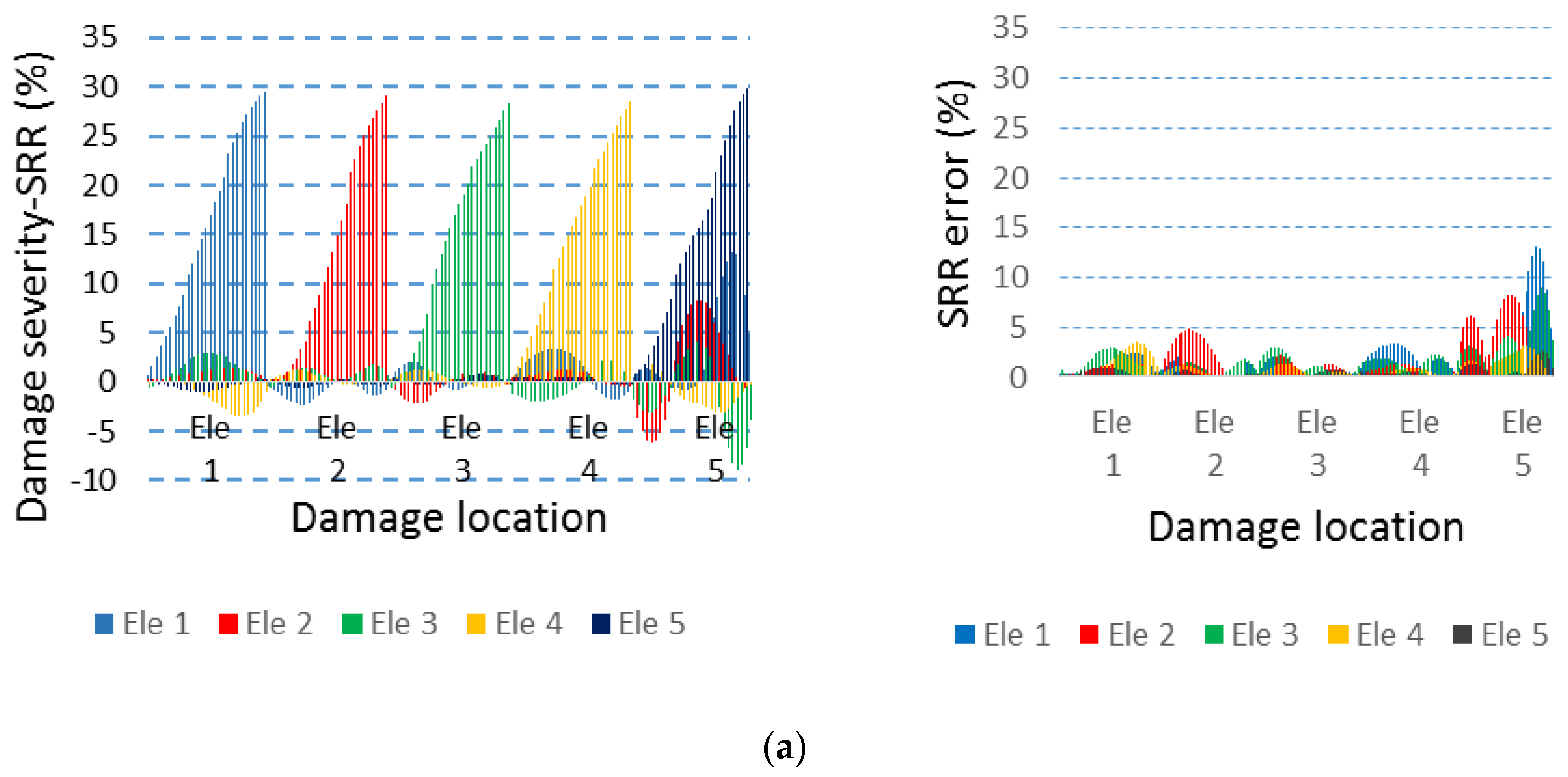
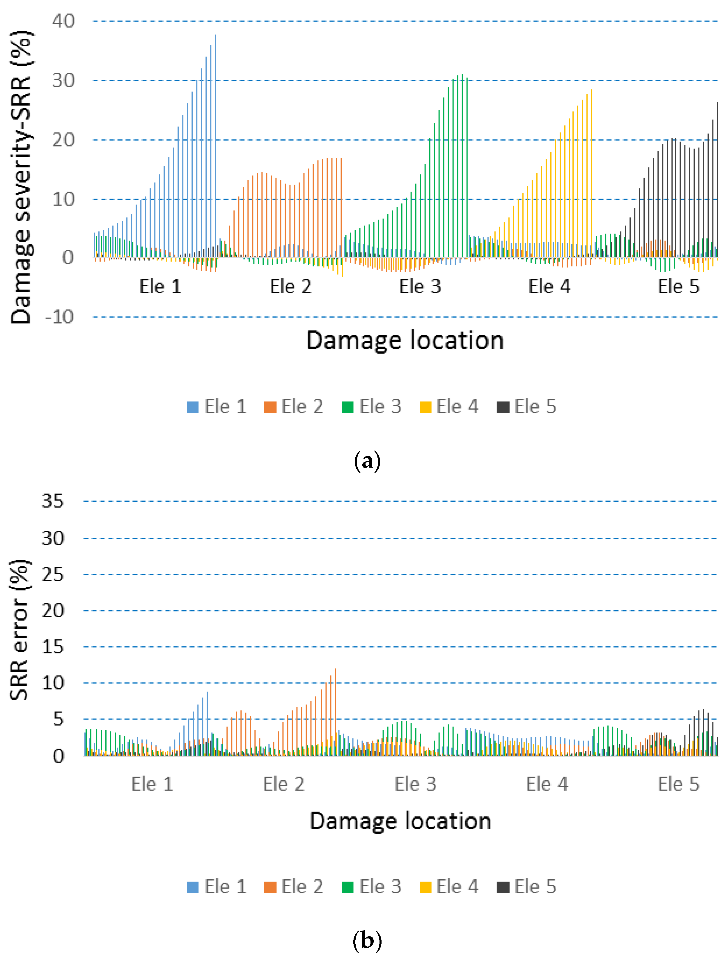
4.4. Robustness Against Noise

Robustness against measurement noise is a key factor for assessing the performance of the damage detection methods [56,57]. The capability of the proposed model to identify damage in noisy conditions is examined by using noisy acceleration responses to simulate actual measurements. The noisy acceleration response is elaborated by adding random Gaussian white noise to the acceleration response obtained from the numerical simulation of the bridge. The noise intensity is quantified by the signal-to-noise ratio (SNR):

$$SNR=20{\log }_{10}\frac{A_S}{A_N}$$

(16)

where $A_S$ and $A_N$ denote the root mean squares of the numerical acceleration response and the noise, respectively. Three high noise levels of SNR = 10 dB, 20 dB, and 30 dB are considered to be used in the analysis of damage identification. At each noise level, the hierarchical neural network model is implemented, with the identification results presented in Figure 10a–c for SNR = 10 dB, 20 dB, and 30 dB, respectively. From the figures, (i) damage location can be discriminated by the model, with errors merely obstructing the judgment in some minor damaged cases; (ii) the results in the noisy conditions show that the model gives an excellent prediction of damage severity, even better than that for the noise-free condition. The effect of noise on damage identification is indicated by the MSE and maximum error, given in

Table 4. Mean square error (MSE) of damage identification in noisy conditions.

Noise	SNR (dB)
	10	20	30	$\mathrm{\infty }$
MSE	4.892	4.94	7.138	3.309
Maximum error	13.1	7.048	10.462	7.044

. From the MSE, we can see that this model still functions in noisy conditions with quite a low error; from the maximum error, it is evident that errors are mostly controlled below the medium level, so that they may only interfere with the identification of minor damage. Therefore, conclusions can be obtained that the proposed hierarchical neural network model can locate and quantify damage in the bridge with great accuracy and strong robustness against noise.

The merit of the robustness against noise of the proposed model is primarily attributed to two factors, i.e., the WPT and the NLPCA: ① WPT. The WPT is an integral transform that has the function of denoising. Moreover, a WPNE resulting from the WPT is formed with the summation of wavelet packet node coefficients squared, which is an operation of assimilating noise. ② NLPCA. For some WPNEs of lower magnitude, they are commonly dominated by noise. Such WPNEs can be almost eliminated by the NLPCA due to their insignificance when conducting NLPCA for feature extraction, resulting in the reduction of noise. The two factors endow the proposed model with the merit of robustness against noise.

5. Comparison with Traditional Methods

The performance of the proposed model is compared to that of a traditional neural-network-based damage assessment method that integrates the general linear PCA and back-propagation neural networks (BPNNs) to identify structural damage [58]. By the way of illustration, this method is used to re-perform the procedure of identifying damage in the bridge in noisy condition. As an alternative to the NLPCA, the PCA is employed to extract damage features from the WPNEs, and then the BPNNs are utilized to recognize damage patterns. Fed with the extracted damage features using PCA, the BPNNs predict the location and severity of the damage, giving the results of the damage identification shown in Figure 11. The results of damage prediction measured by MSE is 5.365 and by maximum error is 12.763. Conspicuously, this traditional model does not identify the severity of the damage with great accuracy. In particular, a relatively significant error of damage identification occurs in the cases whose damage is located in Ele 2 and Ele 5. By comparing Figure 11 with Figure 9, it can be easily seen that the proposed hierarchical identification model assesses the damage with greater accuracy, the performance of which is superior to that of the traditional method. This conclusion is further verified quantitatively by much lower magnitude of MSE and smaller value of maximum error for the proposed model than the traditional one for other cases. The comparison between the two methods demonstrates the great significance and effectiveness of the proposed hierarchical neural network based model.

6. Concluding Remarks

This study proposes a hierarchical neural network model for intelligent damage identification of bridge structures. This model features the synergetic functions of AANNs in extracting damage features from WPNEs, together with the functions of LMNNs in recognizing damage patterns. The model is applied to damage identification in a three-span bridge structure, with its high accuracy of identifying the location and severity of damage and its strong robustness against noise substantiated. The marked strength of the model in portraying damage is attributed to three factors: (i) The WPNEs contain much richer damage information than some traditional modal features, in that the WPNEs carry not only modal damage information but also non-modal damage information; (ii) Damage features, i.e., NPCs, extracted from WPNEs using AANNs, inherit the advantages of both WPT in denoising and NLPCA in accommodating noise. Firstly, the noise is spread during the wavelet packet decomposition, and their effects are greatly weakened during this procedure. Secondly, using NLPCA to process the energy can also remove a part of the noise as this technique omitting some less important information of the original data. Hence, the damage features can characterize damage in severely noisy conditions; (iii) LMNNs are powerful in capturing the underlying relations between damage features and damage states, providing the possibility of recognizing damage patterns efficiently. The proposed model provides a prototype for creating effective technologies to identify damage intelligently in realistic, complex engineering structures.

References

1. Sohn, H.; Farrar, C.R.; Hemez, F.M. A Review of Structural Health Monitoring Literature: 1996–2001; LA-13976-MS; Los Alamos National Laboratory: Los Alamos, NM, USA, 2003. [Google Scholar]
2. Farrar, C.R.; Worden, K. An introduction to structural health monitoring. Philos. Trans. R. Soc. A Math. Phys. Eng. Sci. 2007, 365, 303–315. [Google Scholar] [CrossRef] [PubMed]
3. Ou, J.P.; Li, H. Structural health monitoring in mainland China: Review and future trends. Struct. Health Monit. 2010, 9, 219–231. [Google Scholar]
4. Ciang, C.C.; Lee, J.R.; Bang, H.J. Structural health monitoring for a wind turbine system: A review of damage detection methods. Meas. Sci. Technol. 2008, 19, 310–314. [Google Scholar] [CrossRef]
5. Yan, Y.J.; Cheng, L.; Wu, Z.Y. Development in vibration-based structural damage detection technique. Mech. Syst. Signal Proc. 2007, 21, 2198–2211. [Google Scholar] [CrossRef]
6. Yan, G.; Duan, Z.; Ou, J.P. Review on structural damage detection based on vibration data. Earthq. Eng. Eng. Vib. 2007, 27, 95–103. [Google Scholar]
7. Fan, W.; Qiao, P.Z. Vibration-based damage identification methods: A review and comparative study. Struct. Health Monit. 2010, 9, 83–111. [Google Scholar]
8. Su, Z.Q.; Ye, L.; Lu, Y. Guided Lamb waves for identification of damage in composite structures: A review. J. Sound Vib. 2006, 295, 753–780. [Google Scholar] [CrossRef]
9. Zumpano, G.; Meo, M. A new damage detection technique based on wave propagation for rails. Int. J. Solids Struct. 2006, 43, 1023–1046. [Google Scholar] [CrossRef]
10. Ostachowicz, W. Damage detection of structures using spectral finite element method. Comput. Struct. 2008, 86, 454–462. [Google Scholar] [CrossRef]
11. Vakil-Baghmisheh, M.T.; Peimani, M.; Sadeghi, M.H. Crack detection in beam-like structures using genetic algorithms. Appl. Soft Comput. 2008, 8, 1150–1160. [Google Scholar] [CrossRef]
12. Lam, H.F.; Yuen, K.V.; Beck, J.L. Structural health monitoring via measured Ritz vectors utilizing artificial neural networks. Comput. Aided Civ. Infrastruct. Eng. 2006, 21, 232–241. [Google Scholar] [CrossRef]
13. Ding, Z.C.; Cao, M.S.; Jia, H.L.; Pan, L.X.; Xu, H. Structural dynamics-guided hierarchical neural-networks scheme for locating and quantifying damage in beam-type structures. J. Vibroeng. 2014, 16, 3595–3608. [Google Scholar]
14. Mehrjoo, M.; Khaji, N. Ghafory-Ashtiany, Application of genetic algorithm in crack detection of beam-like structures using a new cracked Euler–Bernoulli beam element. Appl. Soft Comput. 2013, 13, 867–880. [Google Scholar] [CrossRef]
15. Beena, P.; Ganguli, R. Structural damage detection using fuzzy cognitive maps and Hebbian learning. Appl. Soft Comput. 2011, 11, 1014–1020. [Google Scholar] [CrossRef]
16. Cao, M.S.; Qiao, P.Z.; Ren, Q.W. Improved hybrid wavelet neural network methodology for time-varying behavior prediction of engineering structures. Neural Comput. Appl. 2009, 18, 821–832. [Google Scholar] [CrossRef]
17. Hossain, M.S.; Ong, Z.C.; Ismail, Z.; Noroozi, S.; Khoo, S.Y. Artificial neural networks for vibration based inverse parametric identifications: A review. Appl. Soft Comput. 2017, 52, 203–219. [Google Scholar] [CrossRef]
18. Hakim, S.J.S.; Razak, H.A. Modal parameters based structural damage detection using artificial neural networks—A review. Smart Struct. Syst. 2014, 14, 159–189. [Google Scholar] [CrossRef]
19. Worden, K.; Burrows, A.P. Optimal sensor placement for fault detection. Eng. Struct. 2001, 23, 885–901. [Google Scholar] [CrossRef]
20. Worden, K.; Ball, A.D.; Tomlinson, G.R. Fault location in structures using neural networks. In Proceedings of the 75th Meeting of the AGARD Structures and Materials Panel on Smart Structures for Aircraft and Spacecraft, Lindau, Germany, 5–7 October 1992; pp. 1–9. [Google Scholar]
21. Ni, Y.Q.; Wang, B.S.; Ko, J.M. Constructing input vectors to neural networks for structural damage identification. Smart Mater. Struct. 2002, 11, 825–833. [Google Scholar] [CrossRef]
22. Zubaydi, A.; Haddara, M.R.; Swamidas, A.S.J. Damage identification in a ship’s structure using neural networks. Ocean Eng. 2002, 29, 1187–1200. [Google Scholar] [CrossRef]
23. Sahoo, B.; Maity, D. Damage assessment of structures using hybrid neuro-genetic algorithm. Appl. Soft Comput. 2007, 7, 89–104. [Google Scholar] [CrossRef]
24. Hakim, S.J.S.; Razak, H.A. Frequency response function-based structural damage identification using artificial neural networks—A review. Res. J. Appl. Sci. Eng. Technol. 2014, 7, 1750–1764. [Google Scholar] [CrossRef]
25. Cao, M.S.; Qiao, P.Z. Integrated wavelet transform and its application to vibration mode shapes for the damage detection of beam-type structures. Smart Mater. Struct. 2008, 17, 6777–6790. [Google Scholar] [CrossRef]
26. Hou, Z.K.; Noori, M.N.; Amand, R.S. Wavelet-based approach for structural damage detection. J. Eng. Mech. 2000, 126, 677–683. [Google Scholar] [CrossRef]
27. Taha, M.M.R. Wavelet transform for structural health monitoring: A compendium of uses and features. Struct. Health Monit. 2006, 5, 267–295. [Google Scholar] [CrossRef]
28. Cao, M.S.; Cheng, L.; Su, Z.Q. A multi-scale pseudo-force model in wavelet domain for identification of damage in structural components. Mech. Syst. Signal Proc. 2012, 28, 638–659. [Google Scholar] [CrossRef]
29. Yen, G.G.; Lin, K.C. Wavelet packet feature extraction for vibration monitoring. IEEE Trans. Ind. Electron. 2000, 47, 650–667. [Google Scholar] [CrossRef]
30. Han, J.G.; Ren, W.X.; Sun, Z.S. Wavelet packet based damage identification of beam structures. Int. J. Solids Struct. 2005, 42, 6610–6627. [Google Scholar] [CrossRef]
31. Law, S.S.; Zhu, X.Q.; Tian, Y.J. Statistical damage classification method based on wavelet packet analysis. Struct. Eng. Mech. 2013, 46, 459–486. [Google Scholar] [CrossRef]
32. Jiang, X.; Mahadevan, S.; Adeli, H. Bayesian wavelet packet denoising for structural system identification. Struct. Control Health Monit. 2007, 14, 333–356. [Google Scholar] [CrossRef]
33. Ravanfar, S.A.; Razak, H.A.; Ismail, Z. A hybrid wavelet based–approach and genetic algorithm to detect damage in beam-like structures without baseline data. Exp. Mech. 2016, 56, 1–16. [Google Scholar] [CrossRef]
34. Chiariotti, P.; Martarelli, M.; Revel, G.M. Delamination detection by Multi-Level Wavelet Processing of Continuous Scanning Laser Doppler Vibrometry data. Opt. Lasers Eng. 2017. [Google Scholar] [CrossRef]
35. Asgarian, B.; Aghaeidoost, V.; Shokrgozar, H.R. Damage detection of jacket type offshore platforms using rate of signal energy using wavelet packet transform. Mar. Struct. 2016, 45, 1–21. [Google Scholar] [CrossRef]
36. Yam, L.H.; Yan, Y.J.; Jiang, J.S. Vibration-based damage detection for composite structures using wavelet transform and neural network identification. Compos. Struct. 2003, 60, 403–412. [Google Scholar] [CrossRef]
37. Zhu, F.; Deng, Z.; Zhang, J. An integrated approach for structural damage identification using wavelet neuro-fuzzy model. Expert Syst. Appl. 2013, 40, 7415–7427. [Google Scholar] [CrossRef]
38. Diao, Y.S.; Li, H.J.; Wang, Y. A two-step structural damage detection approach based on wavelet packet analysis and neural network. In Proceedings of the IEEE International Conference on Machine Learning and Cybernetics, 13–16 August 2006; pp. 3128–3133. [Google Scholar]
39. Taha, M.M.R. A neural-wavelet technique for damage identification in the ASCE benchmark structure using phase II experimental data. Adv. Civ. Eng. 2010, 2010, 1–13. [Google Scholar] [CrossRef]
40. Yan, G.R.; Duan, Z.D.; Ou, J.P. Structural damage detection by wavelet transform and probabilistic neural network. Smart Struct Mater. 2005, 5765, 892–900. [Google Scholar]
41. Evagorou, D.; Kyprianou, A.; Lewin, P.L. Feature extraction of partial discharge signals using the wavelet packet transform and classification with a probabilistic neural network. IET Sci. Meas. Technol. 2010, 4, 177–192. [Google Scholar] [CrossRef]
42. Torres-Arredondo, M.A.; Buethe, I.; Tibaduiza, D.A. Damage detection and classification in pipework using acousto-ultrasonics and non-linear data-driven modelling. J. Civ. Struct. Health Monit. 2013, 3, 297–306. [Google Scholar] [CrossRef]
43. Sahin, M.; Shenoi, R.A. Quantification and localization of damage in beam-like structures by using artificial neural networks with experimental validation. Eng. Struct. 2003, 25, 1785–1802. [Google Scholar] [CrossRef]
44. Jeyasehar, C.A.; Sumangala, K. Nondestructive evaluation of prestressed concrete beams using an artificial neural network (ANN) approach. Struct. Health Monit. 2006, 5, 313–323. [Google Scholar] [CrossRef]
45. Chakraverty, S.; Gupta, P.; Sharma, S. Neural network-based simulation for response identification of two-storey shear building subject to earthquake motion. Neural Comput. Appl. 2010, 19, 367–375. [Google Scholar] [CrossRef]
46. Law, S.S.; Li, X.Y.; Zhu, X.Q. Structural damage detection from wavelet packet sensitivity. Eng. Struct. 2005, 27, 1339–1348. [Google Scholar] [CrossRef]
47. Gao, R.X.; Yan, R.Q. Wavelet Packet Transform-Theory and Applications for Manufacturing; Springer: Berlin, Germany, 2011. [Google Scholar]
48. Kruger, U.; Zhang, J.; Xie, L. Developments and applications of nonlinear principal component analysis—A review. Lect. Notes Comput. Sci. Eng. 2008, 58, 1–43. [Google Scholar]
49. Cao, M.S.; Pan, L.X.; Gao, Y.F. Neural network ensemble-based parameter sensitivity analysis in civil engineering systems. Neural Comput. Appl. 2015, 26, 1–8. [Google Scholar] [CrossRef]
50. Kramer, M.A. Nonlinear principal component analysis using autoassociative neural networks. AICHE J. 1991, 37, 233–243. [Google Scholar] [CrossRef]
51. Sun, Z.; Chang, C.C. Structural damage assessment based on wavelet packet transform. J. Struct. Eng. 2002, 128, 1354–1361. [Google Scholar] [CrossRef]
52. Sohn, H. Effects of environmental and operational variability on structural health monitoring. Philos. Trans. R. Soc. A Math. Phys. Eng. Sci. 2007, 365, 539–560. [Google Scholar] [CrossRef] [PubMed]
53. Sohn, H.; Worden, K.; Farrar, C.R. Statistical damage classification under changing environmental and operational conditions. J. Intell. Mater. Syst. Struct. 2002, 13, 561–574. [Google Scholar] [CrossRef]
54. Suratgar, A.A.; Tavakoli, M.B.; Hoseinabadi, A. Modified Levenberg-Marquardt method for neural networks training. World Acad. Sci. Eng. Technol. 2005, 6, 46–48. [Google Scholar]
55. Maeck, J.; Peeters, B.; Deroeck, G. Damage identification on the Z24 bridge using vibration monitoring. Smart Mater. Struct. 2001, 10, 512–517. [Google Scholar] [CrossRef]
56. Reynders, E.; Wursten, G.; Roeck, G.D. Output-only structural health monitoring in changing environmental conditions by means of nonlinear system identification. Struct. Health Monit. 2013, 13, 82–93. [Google Scholar] [CrossRef]
57. Spiridonakos, M.D.; Chatzi, E.N.; Sudret, B. Polynomial chaos expansion models for the monitoring of structures under operational variability. ASCE-ASME J. Risk Uncertain. Eng. Syst. A Civ. Eng. 2016, 2. [Google Scholar] [CrossRef]
58. Sun, Y. Combined neural network and PCA for complicated damage detection of bridge. In Proceedings of the International Conference on Natural Computation, Tianjin, China, 14–16 August 2009; pp. 524–528. [Google Scholar]
Figure 1. Schematic of wavelet packet transform (WPT) of a time-domain signal. A: approximate component signal; D: detail component signal.
Applsci 07 00391 g001
Figure 2. Auto-associative neural networks (AANNs) for damage feature extraction from wavelet packet node energies (WPNEs). (A) mapping layer; (B) bottleneck layer; (C) remapping layer.
Applsci 07 00391 g002
Figure 3. Levenberg-Marquardt neural networks (LMNNs) for damage pattern recognition. (A) input layer; (B) hidden layer; (C) output layer.
Applsci 07 00391 g003
Figure 4. Hierarchical neural network model.
Applsci 07 00391 g004
Figure 5. Three-span continuous bridge.
Applsci 07 00391 g005
Figure 6. Extracted nonlinear principle components (NPCs) from wavelet packet node energies (WPNEs) using AANNs. (a) WPNEs; (b) Normalized WPNEs; (c) Normalized NPCs.
Applsci 07 00391 g006
Figure 7. Visualization of the capability of NPCs to characterize damage by a progressively zoomed-in cube.
Applsci 07 00391 g007
Figure 8. Identification of damage in Ele 1 of the bridge. (a) Damage estimate; (b) Target output; (c) Damage identification error.
Applsci 07 00391 g008
Figure 9. Identification of damage in the bridge in noise-free condition. (a) Damage estimate; (b) Target output; (c) Damage identification error.
Applsci 07 00391 g009
Figure 10. Identification of damage in the bridge in severely noisy conditions. (a) signal-to-noise ratio (SNR) = 10 dB; (b) SNR = 20 dB; (c) SNR = 30 dB.
Applsci 07 00391 g010aApplsci 07 00391 g010b
Figure 11. Identification of damage using a typical method in the noise-free condition. (a) Damage estimate; (b) Identification error.
Applsci 07 00391 g011