
A Timed Colored Petri Net Simulation-Based Self-Adaptive Collaboration Method for Production-Logistics Systems


Abstract
:1. Introduction
- (1)
- How can the advantages of IoT and CC technology be leveraged to model the behaviors of key production and logistics equipment and make the equipment ‘smart’? Generally, key equipment such as machines and AGVs simply execute the commands of the preset programs or workers. The equipment is not aware and cannot make decisions based on dynamic changes in the manufacturing environment. Thus, they cannot adjust the schedule according to real-time scenarios.
- (2)
- How can a production-logistics collaboration strategy be designed to undertake active response and self-organizing configuration? In traditional manufacturing systems, the behaviors of both machines and AGVs are event-driven. The logistics task generates after the machine processing is finished. However, this kind of production-logistics system is time-consuming, which may cause high costs.
- (3)
- How can key manufacturing resources be integrated with cloud service platforms to provide the foundations for production-logistics collaboration? Despite the achievements in Industry 4.0 and CPS models, it is not clear how to implement production-logistics collaboration in an FMS. An integrated framework is needed to describe the relationships among different components of the FMS and the cloud service platform.
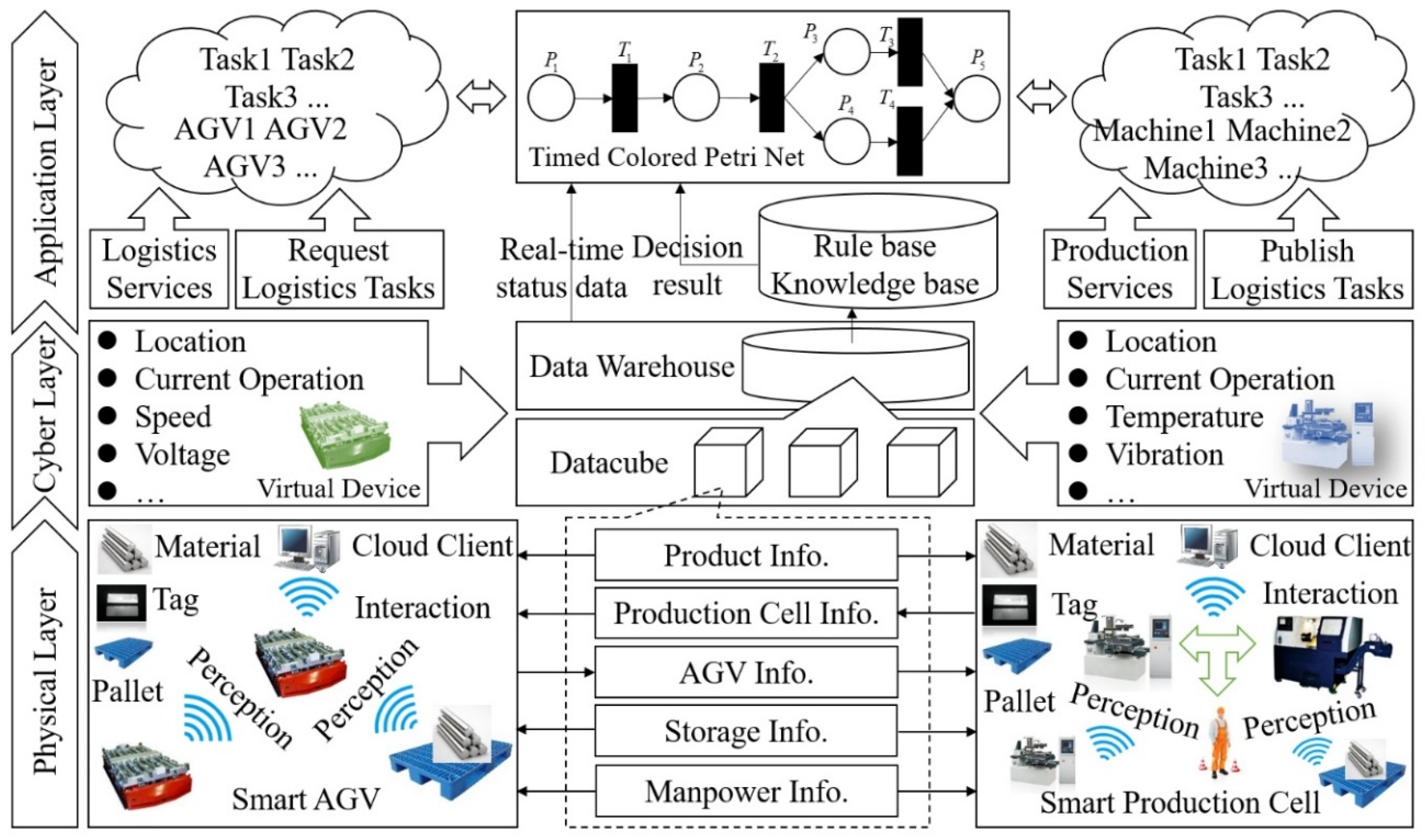
2. Framework
2.1. The Physical Layer
2.2. The Cyber Layer
2.3. The Application Layer
3. Method
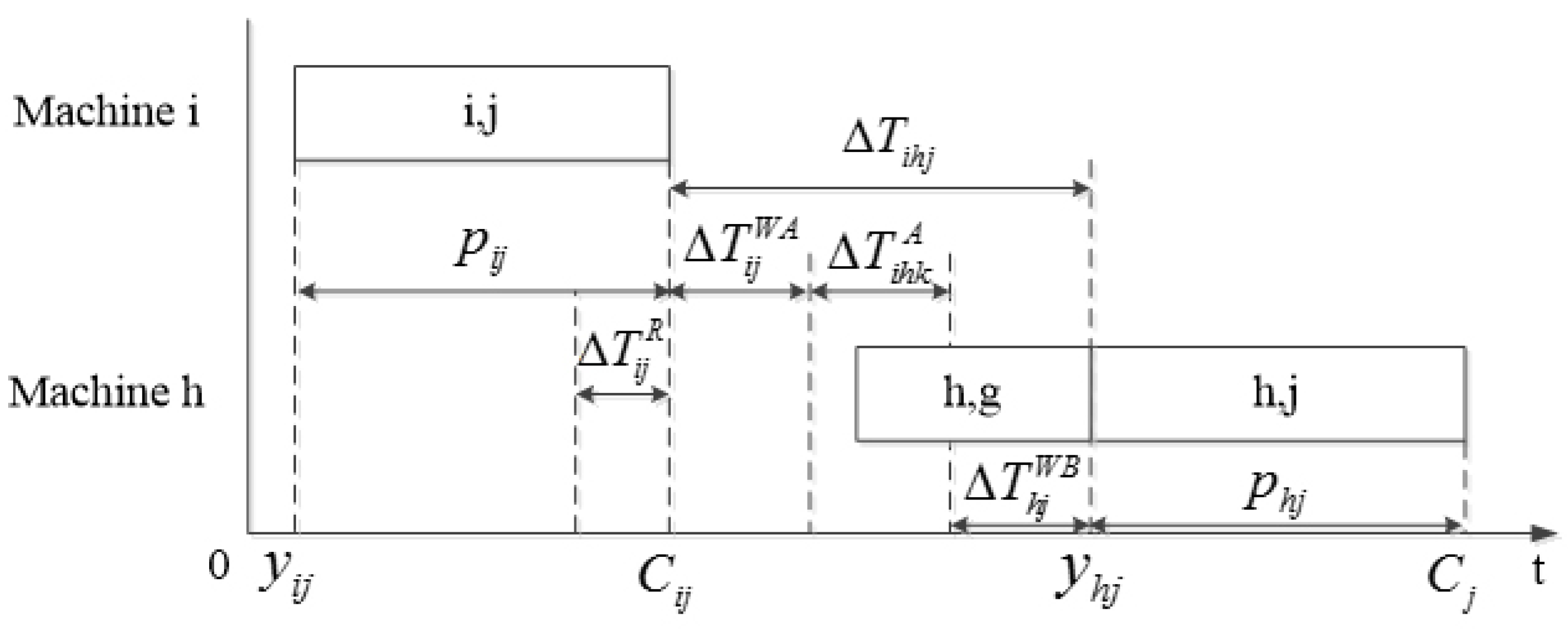
3.1. Problem Definition and Notations
- : machine
- : job
- : an operation that job is processed on machine
- : job should be firstly processed on machine and then on machine
- : current time
- : starting time of operation
- : processing time of operation
- : remaining time of operation
- : priority of logistics task between operation and operation
- : volume of parts transported from machine to machine
- : remaining space of AGV at time
- : path length of road segment
- : speed of AGV
- : time cost of AGV passing road segment
- : time cost of AGV arriving at machine
- : time cost of AGV going from machine to machine
- : total waiting time
- : waiting time between operation and operation
- : waiting time of job on machine before processing
- : waiting time of job on machine after processing
- : makespan
- : completion time of job
- : completion time of operation
- : total electricity consumption
- : electricity consumption of machine
- : electricity consumption of AGV
- : average power of machine when processing
- : average power of machine when idle
- : average power of AGV
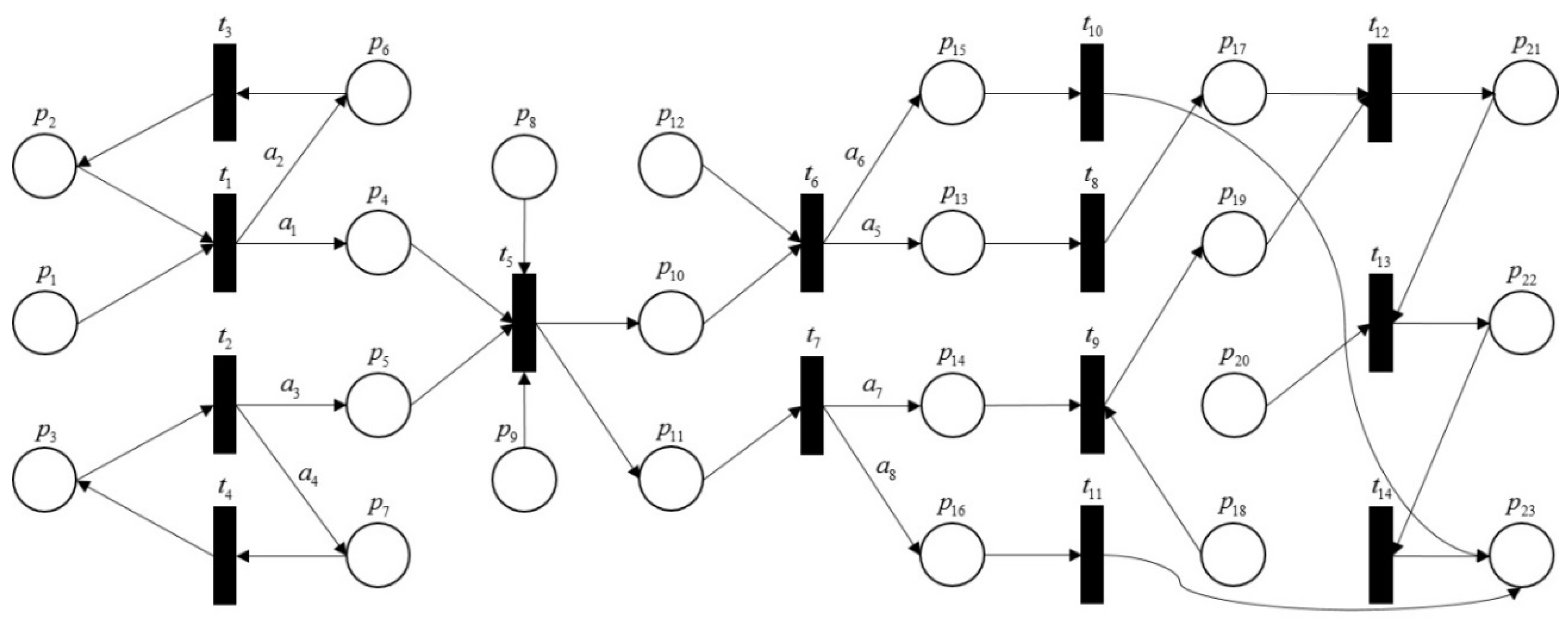
3.2. Timed Colored Petri Net Model
- is a finite set of places.
- is a finite set of transitions, and .
- is a finite set of directed arcs, .
- is a finite set of non-empty color sets.
- is a node function defined from into .
- : is a color set function that assigns a color set to each place.
- : is a guard function that assigns a guard to each transition such that:
- : is an arc expression function that assigns an arc expression to each arc such that:where is the place of .
- : is an initialization function that assigns an initialization expression to each place such that:denotes the type of the variable . denotes a set of variables in the expression .
3.3. Mechanism of Self-Adaptive Collaboration
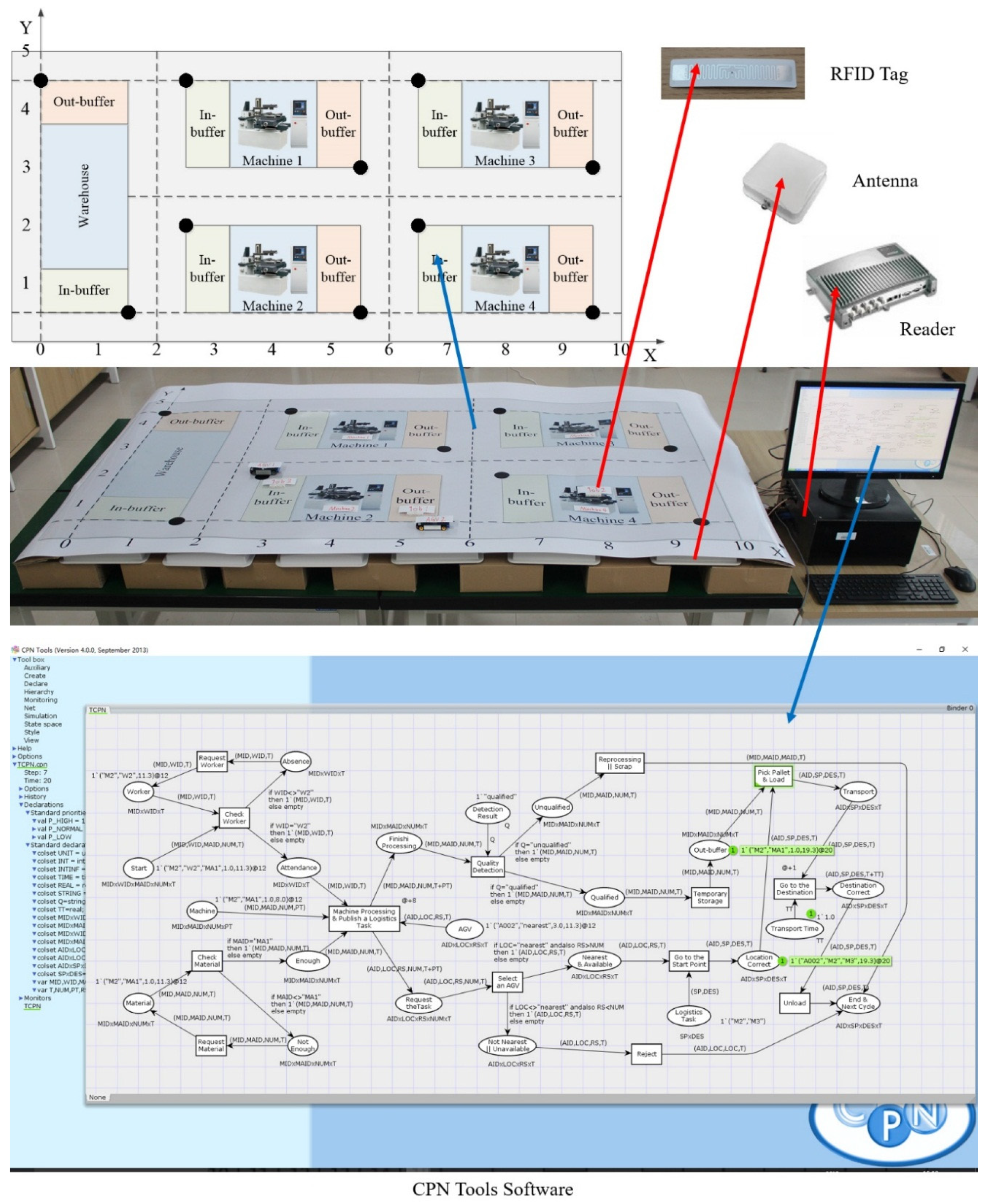
4. Simulation Results
5. Conclusions
Acknowledgments
Author Contributions
Conflicts of Interest
References
- Herrero, D.; Mart, H. Modeling Distributed Transportation Systems Composed of Flexible Automated Guided Vehicles in Flexible Manufacturing Systems. IEEE Trans. Ind. Inform. 2010, 6, 166–180. [Google Scholar] [CrossRef]
- Li, D.X.; He, W.; Li, S. Internet of Things in Industries: A Survey. IEEE Trans. Ind. Inform. 2014, 10, 2233–2243. [Google Scholar]
- Xu, X. From cloud computing to cloud manufacturing. Robot. Comput. Integr. Manuf. 2012, 28, 75–86. [Google Scholar] [CrossRef]
- Zhang, Y.; Qian, C.; Lv, J.; Liu, Y. Agent and cyber-physical system based self-organizing and self-adaptive intelligent shopfloor. IEEE Trans. Ind. Inform. 2017, in press. [Google Scholar] [CrossRef]
- Girbea, A.; Suciu, C.; Nechifor, S.; Sisak, F. Design and implementation of a service-oriented architecture for the optimization of industrial applications. IEEE Trans. Ind. Inform. 2014, 10, 185–196. [Google Scholar] [CrossRef]
- Zhang, Y.F.; Ren, S.; Liu, Y.; Si, S.B. Big data based analysis architecture of complex product manufacturing and maintenance process for sustainable production. J. Clean. Prod. 2017, 142, 626–641. [Google Scholar] [CrossRef]
- Zhang, Y.; Zhang, G.; Wang, J.; Sun, S.; Si, S.; Yang, T. Real-time information capturing and integration framework of the internet of manufacturing things. Int. J. Comput. Integr. Manuf. 2015, 28, 811–822. [Google Scholar] [CrossRef]
- Li, X.; Song, J.; Huang, B. A scientific workflow management system architecture and its scheduling based on cloud service platform for manufacturing big data analytics. Int. J. Adv. Manuf. Technol. 2016, 84, 119–131. [Google Scholar] [CrossRef]
- Um, I.; Cheon, H.; Lee, H. The simulation design and analysis of a flexible manufacturing system with automated guided vehicle system. J. Manuf. Syst. 2009, 28, 115–122. [Google Scholar] [CrossRef]
- Uzam, M.; Zhou, M. An Iterative Synthesis Approach to Petri Net-Based Deadlock Prevention Policy for Flexible Manufacturing Systems. IEEE Trans. Syst. Man Cybern. A Syst. Hum. 2007, 37, 362–371. [Google Scholar] [CrossRef]
- Li, Z.W.; Zhou, M.C.; Wu, N.Q. A survey and comparison of Petri net-based deadlock prevention policies for flexible manufacturing systems. IEEE Trans. Syst. Man Cybern. C Appl. Rev. 2008, 38, 173–188. [Google Scholar]
- Silva, M. Individuals, Populations and fluid approximations: A Petri net based perspective. Nonlinear Anal. Hybrid Syst. 2016, 22, 72–97. [Google Scholar] [CrossRef]
- Wang, S.; You, D.; Wang, C. Optimal supervisor synthesis for petri nets with uncontrollable transitions: A bottom-up algorithm. Inf. Sci. 2016, 363, 261–273. [Google Scholar] [CrossRef]
- Baruwa, O.T.; Piera, M.A. A coloured Petri net-based hybrid heuristic search approach to simultaneous scheduling of machines and automated guided vehicles. Int. J. Prod. Res. 2016, 54, 4773–4792. [Google Scholar] [CrossRef]
- Raj, J.A.; Ravindran, D.; Saravanan, M.; Prabaharan, T. Simultaneous scheduling of machines and tools in multimachine flexible manufacturing systems using artificial immune system algorithm. Int. J. Comput. Integr. Manuf. 2014, 27, 401–414. [Google Scholar] [CrossRef]
- Xia, H.; Li, X.; Gao, L. A hybrid genetic algorithm with variable neighborhood search for dynamic integrated process planning and scheduling. Comput. Ind. Eng. 2016, 102, 99–112. [Google Scholar] [CrossRef]
- Lacomme, P.; Larabi, M.; Tchernev, N. Job-shop based framework for simultaneous scheduling of machines and automated guided vehicles. Int. J. Prod. Econ. 2013, 143, 24–34. [Google Scholar] [CrossRef]
- Qu, T.; Lei, S.P.; Wang, Z.Z.; Nie, D.X.; Chen, X.; Huang, G.Q. IoT-based real-time production logistics synchronization system under smart cloud manufacturing. Int. J. Adv. Manuf. Technol. 2016, 84, 147–164. [Google Scholar] [CrossRef]
- Luo, H.; Wang, K.; Kong, X.T.R.; Lu, S.; Qu, T. Synchronized production and logistics via ubiquitous computing technology. Robot. Comput. Integr. Manuf. 2017, 45, 99–115. [Google Scholar] [CrossRef]
- Li, W.; Zhao, Y.; Lu, S.; Chen, D. Mechanisms and challenges on mobility-augmented service provisioning for mobile cloud computing. IEEE Commun. Mag. 2015, 53, 89–97. [Google Scholar] [CrossRef]
- Lee, J.; Kim, Y.; Kwak, Y.; Zhang, J.; Papasakellariou, A.; Novlan, T.; Sun, C.; Li, Y. LTE-advanced in 3GPP Rel-13/14: An evolution toward 5G. IEEE Commun. Mag. 2016, 54, 36–42. [Google Scholar] [CrossRef]
- Baruwa, O.T.; Piera, M.A.; Guasch, A. TIMSPAT—Reachability graph search-based optimization tool for colored Petri net-based scheduling. Comput. Ind. Eng. 2016, 101, 372–390. [Google Scholar] [CrossRef]
- Baruwa, O.T.; Piera, M.A.; Guasch, A. Deadlock-Free Scheduling Method for Flexible Manufacturing Systems Based on Timed Colored Petri Nets and Anytime Heuristic Search. Int. J. Prod. Res. 2014, 45, 831–846. [Google Scholar] [CrossRef]
- Jensen, K.; Kristensen, L.M. Formal Definition of Timed Coloured Petri Nets. In Coloured Petri Nets; Springer: Berlin/Heidelberg, Germany, 2009; pp. 257–271. [Google Scholar]
- Pinedo, M.L. Machine Scheduling and Job Shop Scheduling. In Planning and Scheduling in Manufacturing and Services; Springer: New York, NY, USA, 2009; pp. 83–115. [Google Scholar]


| Transition | Description of Transitions |
|---|---|
| The transition aims at modeling the check of the worker | |
| The transition aims at modeling the check of the material | |
| The transition aims at modeling requesting the worker | |
| The transition aims at modeling requesting the material | |
| The transition aims at modeling the machine processing and publishing a logistics task | |
| The transition aims at modeling the quality detection | |
| The transition aims at modeling the selection of the AGV | |
| The transition aims at modeling the temporary storage | |
| The transition aims at modeling the selected AGV going to the start point | |
| The transition aims at modeling the reprocessing or the scarp | |
| The transition aims at modeling the rejection of the AGV | |
| The transition aims at modeling picking pallet and loading | |
| The transition aims at modeling the selected AGV going to the destination | |
| The transition aims at modeling the unloading |
| Place | Description of Places |
|---|---|
| A token in this place represents a production task | |
| A token in this place represents a worker | |
| A token in this place represents a material | |
| A token in this place represents the attendance of the worker | |
| A token in this place represents enough materials | |
| A token in this place represents the absence of the worker | |
| A token in this place represents insufficient materials | |
| A token in this place represents the sataus information of a machine | |
| A token in this place represents the sataus information of an AGV | |
| A token in this place represents the finish of the machine processing | |
| A token in this place represents the request to the logistics task | |
| A token in this place represents the detection result | |
| A token in this place represents the qualified WIP | |
| A token in this place represents the nearest and available AGV | |
| A token in this place represents the unqualified WIP | |
| A token in this place represents the remote or unavailable AGV | |
| A token in this place represents an out-buffer | |
| A token in this place represents the selected logistics task | |
| A token in this place represents the correct start point | |
| A token in this place represents the transport time | |
| A token in this place represents the transport to the destination | |
| A token in this place represents the correct destination | |
| A token in this place represents the end and next cycle |
| Color Set | Place |
|---|---|
| colset UNIT = unit; colset INT = int; colset REAL = real; colset STRING = string; | |
| colset MIDxWIDxMAIDxNUMxT = product STRING*STRING*STRING*REAL*REAL timed; | |
| colset MIDxMAIDxNUMxT = product STRING*STRING*REAL*REAL timed; | , , , , , , |
| colset MIDxWIDxT = product STRING*STRING*REAL timed; | , , |
| colset MIDxMAIDxNUMxPT = product STRING*STRING*REAL*REAL timed; | |
| colset AIDxLOCxRSxT = product STRING*STRING*REAL*REAL timed; | , , |
| colset AIDxLOCxRSxNUMxT = product STRING*STRING*REAL*REAL*REAL timed; | |
| colset Q = string; | |
| colset SPxDES = product STRING*STRING; | |
| colset AIDxSPxDESxT = product STRING*STRING*STRING*REAL timed; | , , , |
| colset TT = real; | |
| var MID,WID,MAID,AID,LOC,Q,SP,DES: STRING; var T,NUM,PT,RS,TT: REAL; |
| Jobs | Machine Sequence | Processing Times | Volume |
|---|---|---|---|
| 1 | 1, 2, 3 | 1 | |
| 2 | 2, 1, 4, 3 | 2 | |
| 3 | 1, 2, 4 | 1.5 |
| Task ID | Start Point (X, Y) | Destination (X, Y) | Job ID | Priority | AGV ID | Remaining Space | Waiting Time | Computing Time (s) | ||
|---|---|---|---|---|---|---|---|---|---|---|
| After | Transport | Before | ||||||||
| T0001 | W(0, 4.5) | M1(2.5, 4.5) | 1 | 0-t | A001 | 2 | 0 | 0.5 | 0 | <0.01 |
| T0002 | W(0, 4.5) | M2(2.5, 2) | 2 | 0-t | A002 | 1 | 0 | 1 | 0 | <0.01 |
| T0003 | W(0, 4.5) | M1(2.5, 4.5) | 3 | 10-t | A001 | 0.5 | 0 | 0.5 | 10 | <0.01 |
| T0004 | M1(5.5, 3) | M2(2.5, 2) | 1 | 10-t | A002 | 2 | 0 | 0.8 | 0 | <0.01 |
| T0005 | M2(5.5, 0.5) | M1(2.5, 4.5) | 2 | 14-t | A002 | 1 | 4.1 | 1.4 | 0 | <0.01 |
| T0006 | M1(5.5, 3) | M4(6.5, 2) | 2 | 17-t | A002 | 1 | 0 | 0.4 | 0 | <0.01 |
| T0007 | M1(5.5, 3) | M2(2.5., 2) | 3 | 18-t | A001 | 1.5 | 4 | 0.8 | 0 | <0.01 |
| T0008 | M2(5.5, 0.5) | M3(6.5., 4.5) | 1 | 18-t | A002 | 2 | 0 | 1 | 0 | <0.01 |
| T0009 | M4(9.5, 0.5) | M3(6.5., 4.5) | 2 | 22-t | A002 | 1 | 0 | 1.4 | 0 | <0.01 |
| T0010 | M2(5.5, 0.5) | M4(6.5., 2) | 3 | 25-t | A001 | 1.5 | 0 | 0.5 | 0 | <0.01 |
| KPI | Event-Driven Method | Self-Adaptive Collaboration Method |
|---|---|---|
| Total waiting time | 37.1 | 26.4 |
| Makespan | 36.3 | 30.3 |
| Total electricity consumption | 1035.3 | 993.5 |
© 2017 by the authors. Licensee MDPI, Basel, Switzerland. This article is an open access article distributed under the terms and conditions of the Creative Commons Attribution (CC BY) license ( http://creativecommons.org/licenses/by/4.0/).
Share and Cite
Guo, Z.; Zhang, Y.; Zhao, X.; Song, X. A Timed Colored Petri Net Simulation-Based Self-Adaptive Collaboration Method for Production-Logistics Systems. Appl. Sci. 2017, 7, 235. https://doi.org/10.3390/app7030235
Guo Z, Zhang Y, Zhao X, Song X. A Timed Colored Petri Net Simulation-Based Self-Adaptive Collaboration Method for Production-Logistics Systems. Applied Sciences. 2017; 7(3):235. https://doi.org/10.3390/app7030235
Chicago/Turabian StyleGuo, Zhengang, Yingfeng Zhang, Xibin Zhao, and Xiaoyu Song. 2017. "A Timed Colored Petri Net Simulation-Based Self-Adaptive Collaboration Method for Production-Logistics Systems" Applied Sciences 7, no. 3: 235. https://doi.org/10.3390/app7030235
APA StyleGuo, Z., Zhang, Y., Zhao, X., & Song, X. (2017). A Timed Colored Petri Net Simulation-Based Self-Adaptive Collaboration Method for Production-Logistics Systems. Applied Sciences, 7(3), 235. https://doi.org/10.3390/app7030235