
Measurement and Analysis of Channel Characteristics in Reflective Environments at 3.6 GHz and 14.6 GHz

 , ,
, , 
Abstract
:1. Introduction
- A detailed insight into the channel characteristics of the path loss, RMS (root-mean-square) delay spread and coherence bandwidth in the corridor scenario with the directional antennas at 3.6 GHz and 14.6 GHz frequency bands is presented.
- A comparative analysis is made for statistical metrics of the propagation channel between the two frequency bands.
- The underlying factors that lead to the influence of frequency on the channel characteristics are investigated. It is found that, in the corridor, the differences between the two frequency bands in RMS delay spread are minimal (less than 1 ns). Measurements in the reverberation chamber (RC) verify this inference.
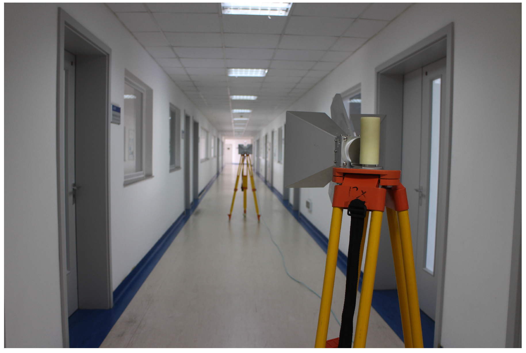
2. Measurements
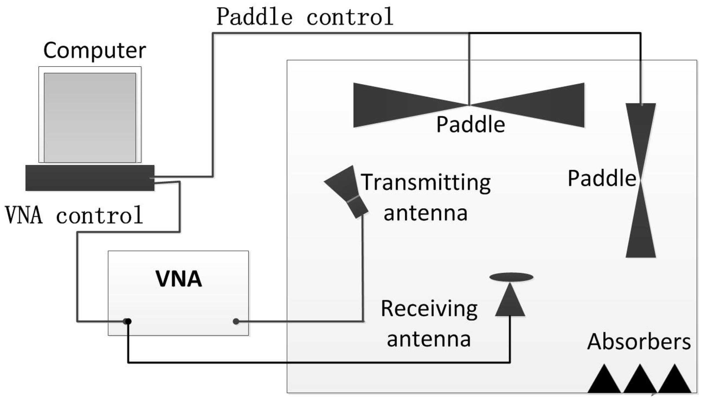
2.1. Measurement System
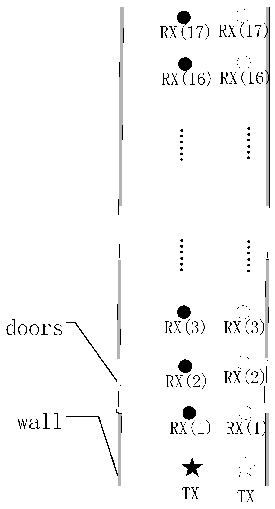
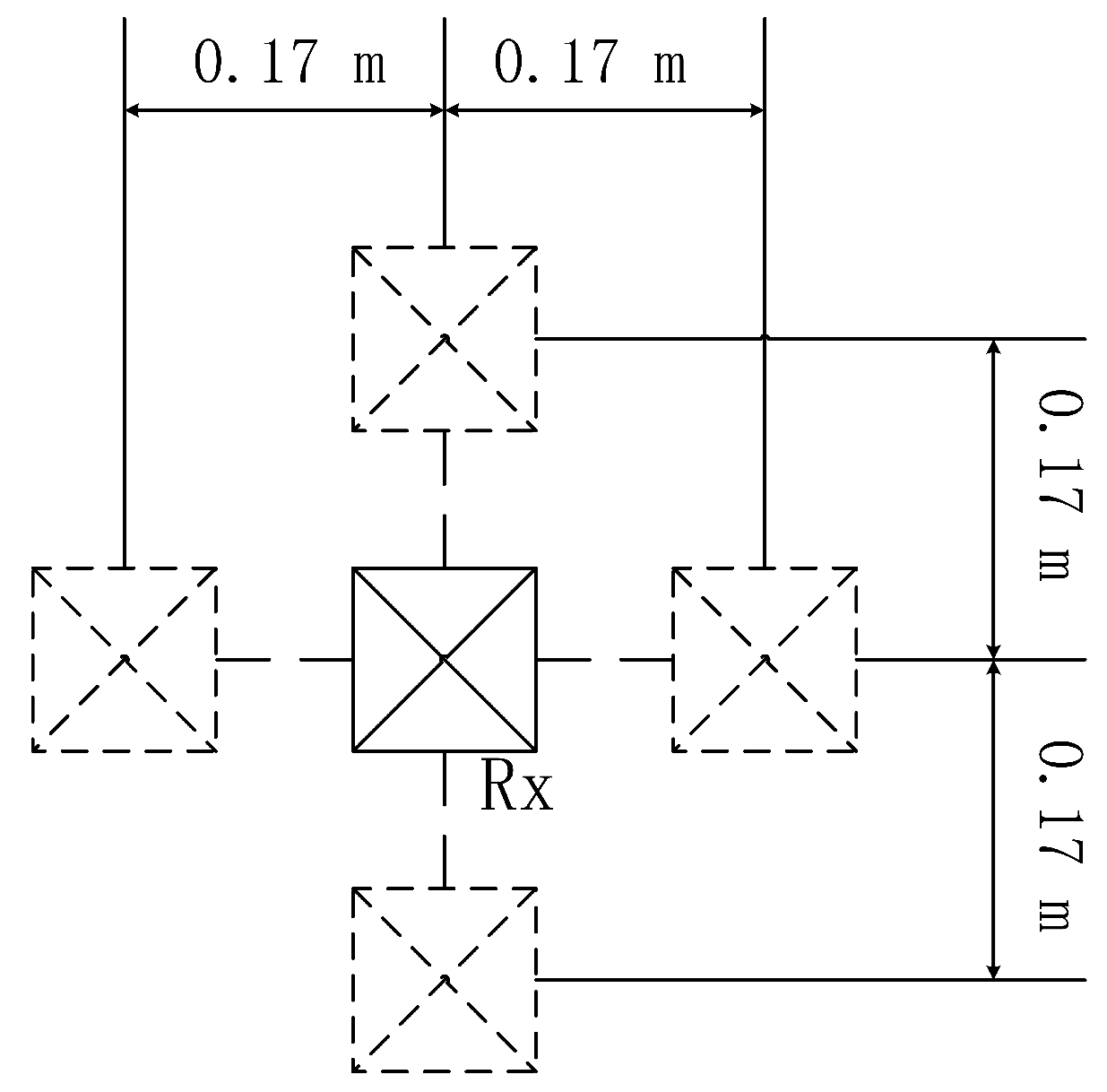
2.2. Measurement Scenario
3. Parameter Extraction and Measurement Results
3.1. Path Loss Exponent and Shadow Fading
3.2. Delay Spread
3.3. Coherence Bandwidth
3.4. Measurement Results
4. Comparative Analysis
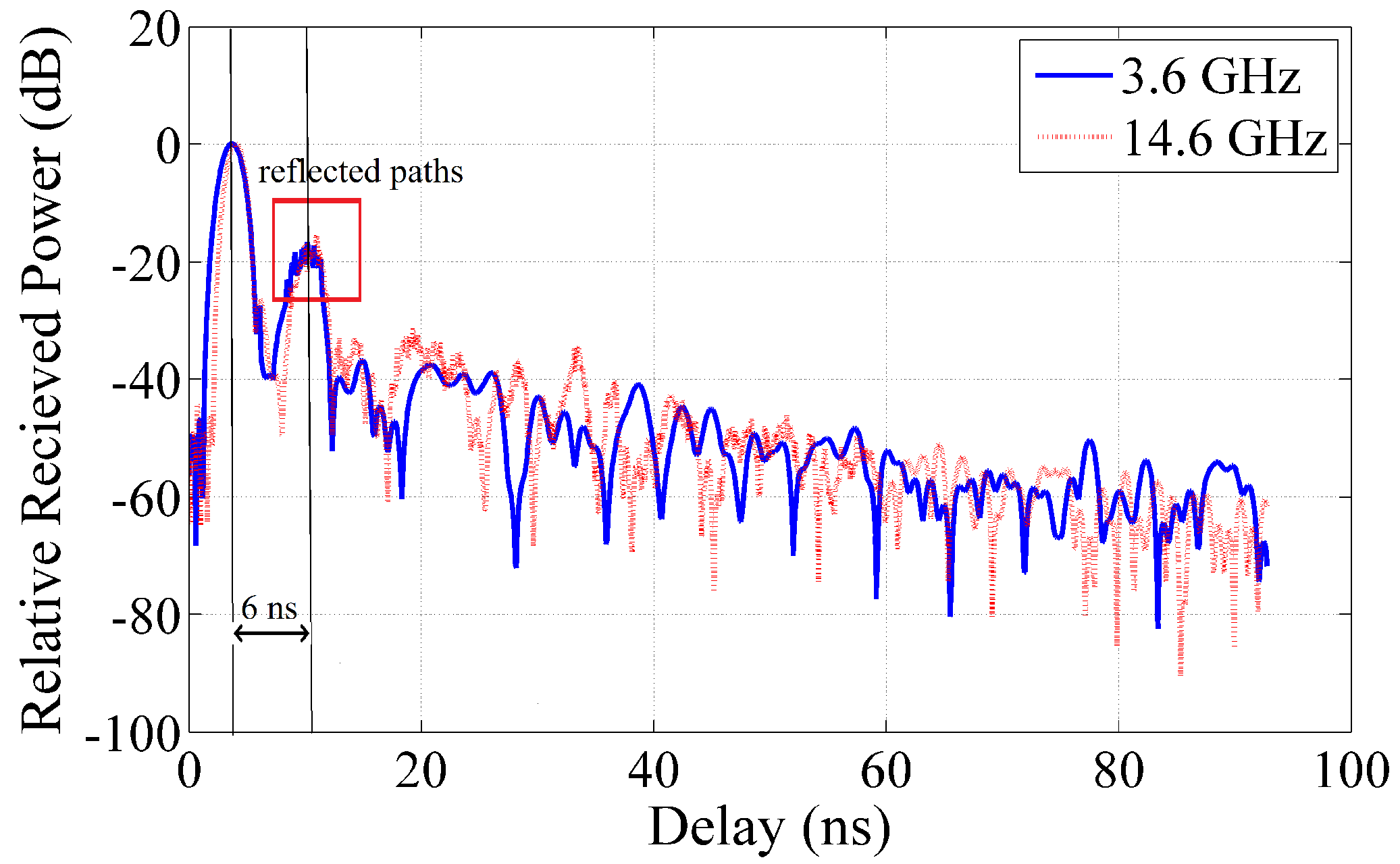
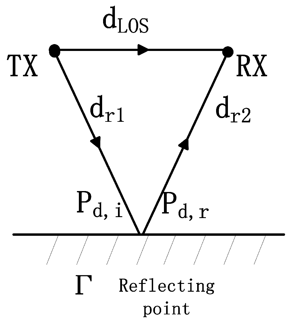
4.1. Example APDPs
4.2. RMS Delay Spread
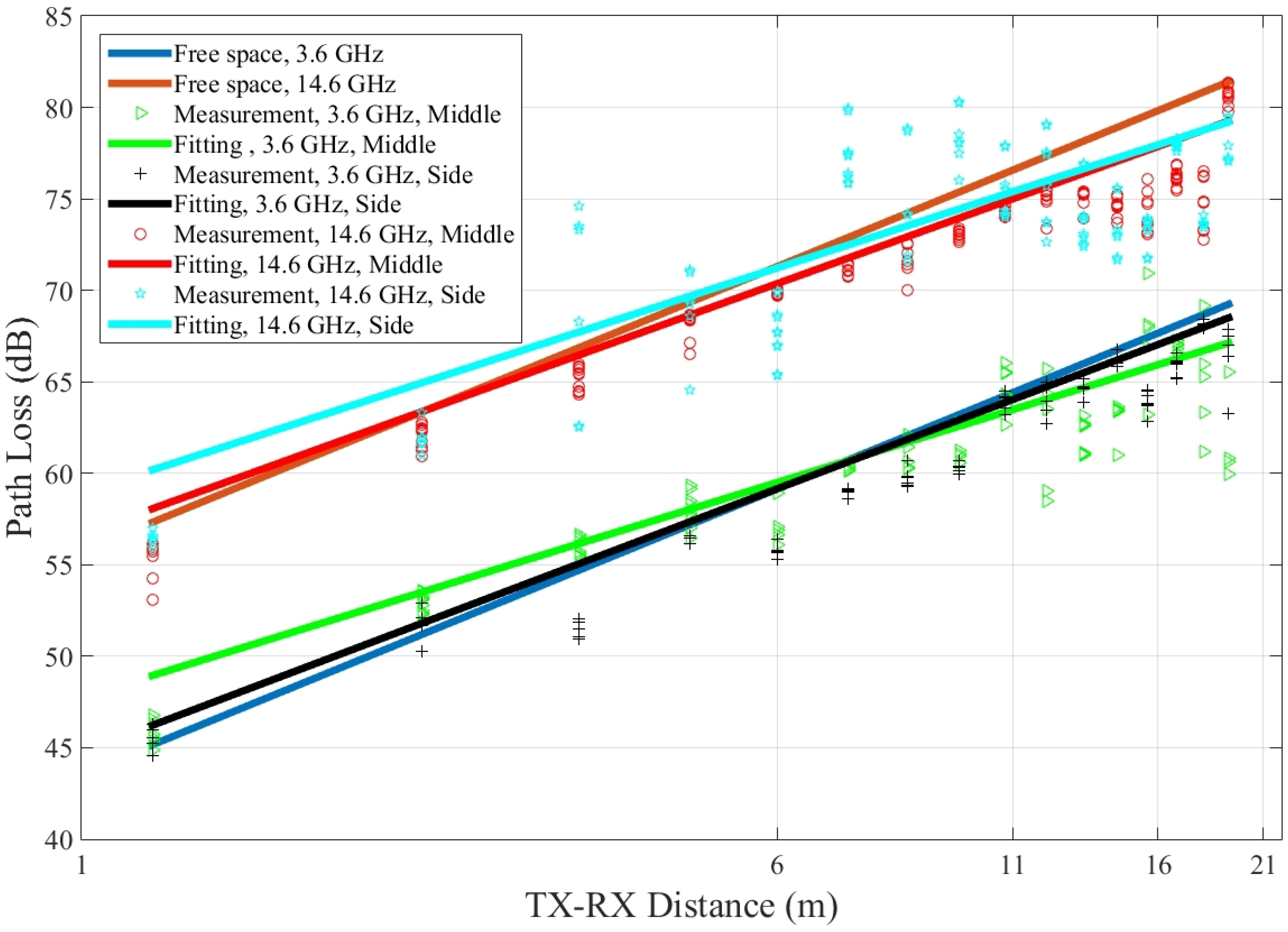
4.3. Path Loss
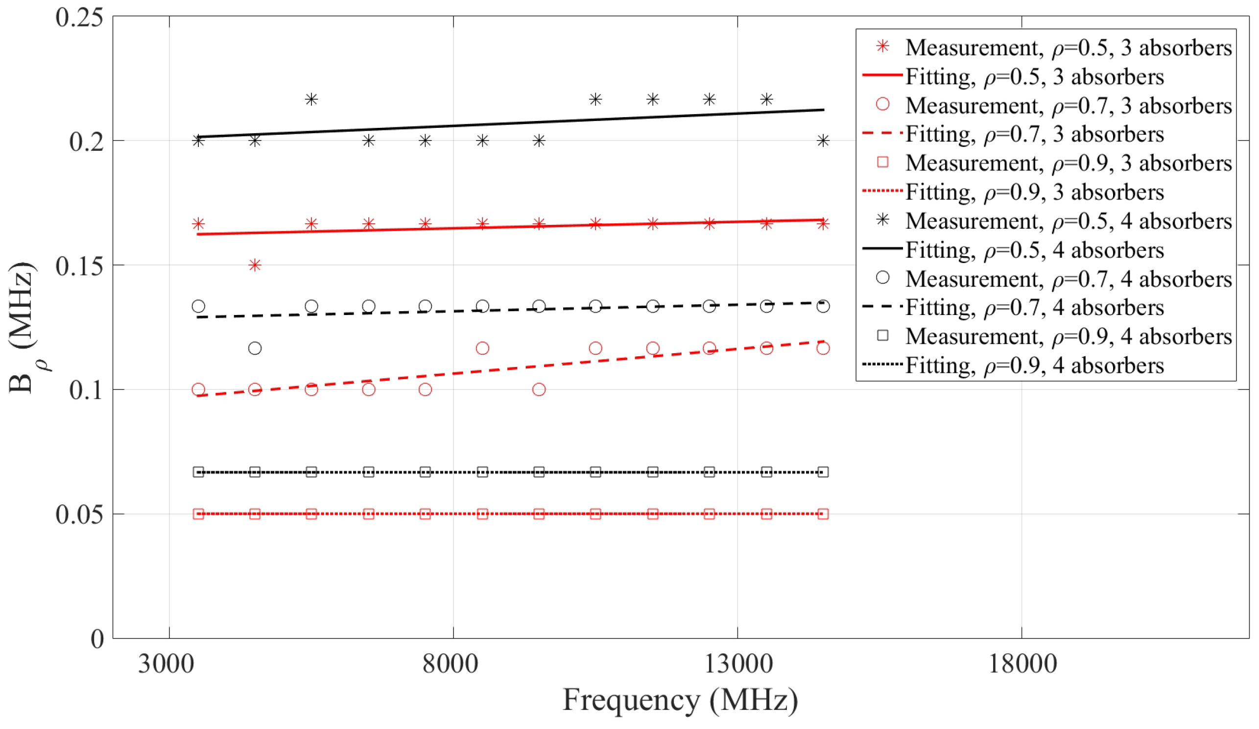
4.4. Coherence Bandwidth
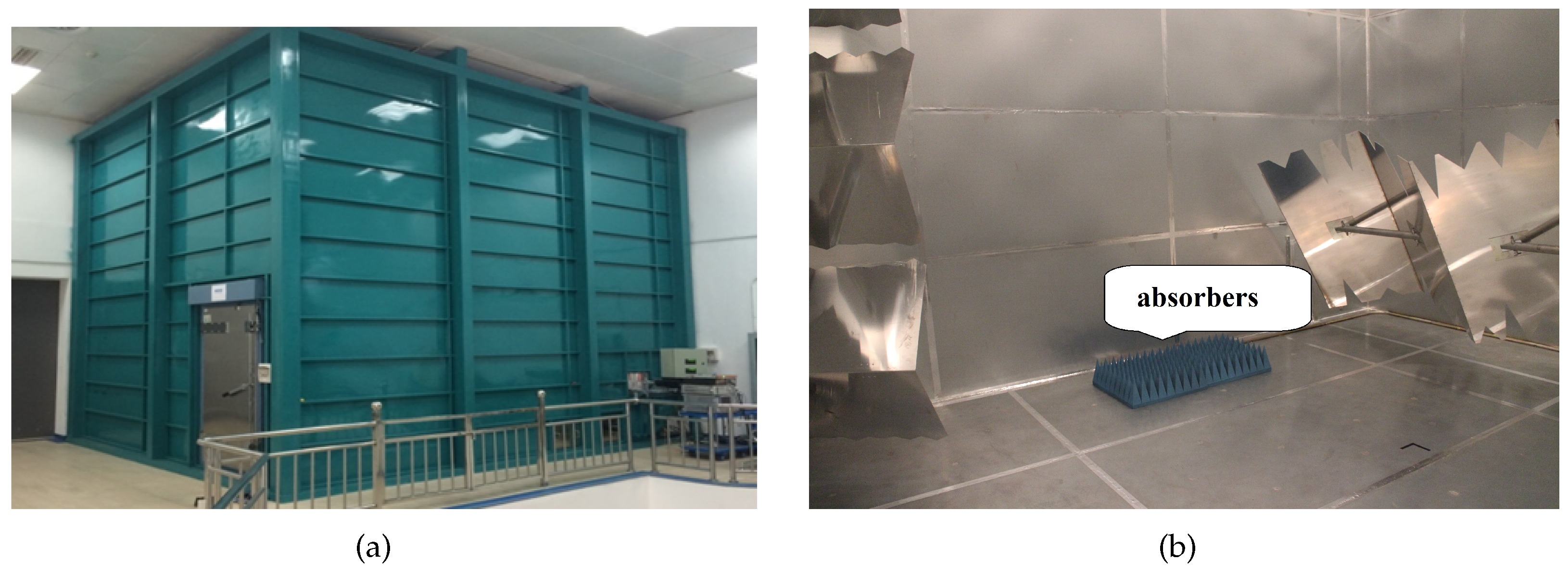
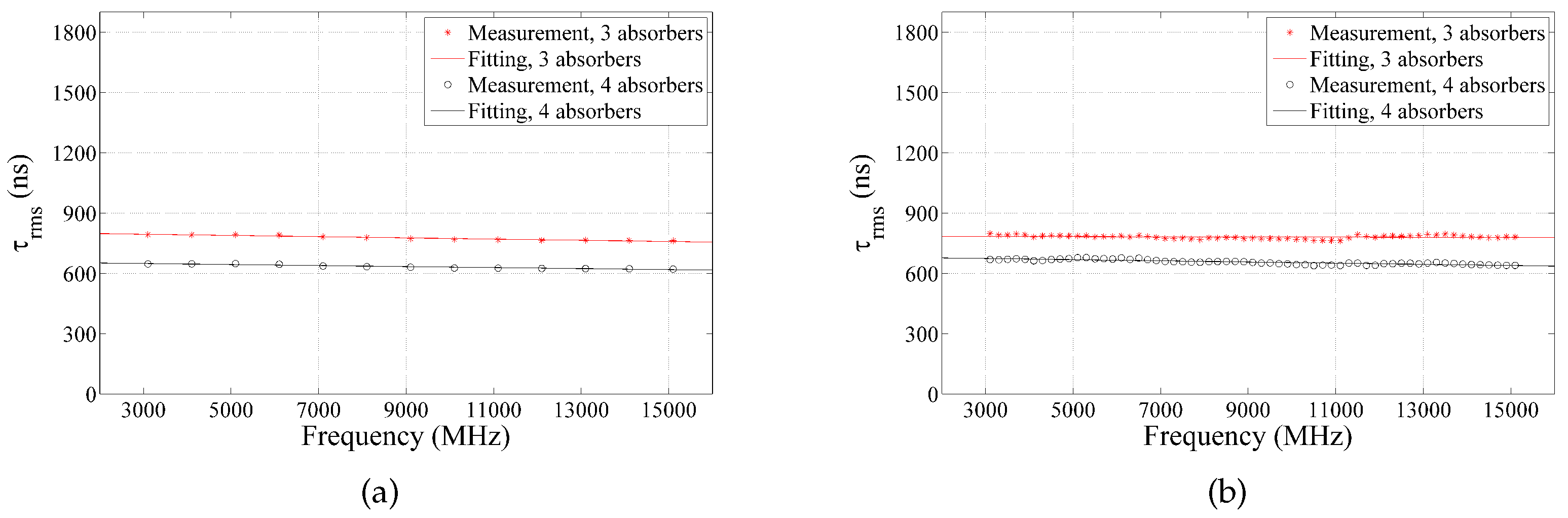
5. Verification in Reverberation Chamber
6. Conclusions
Acknowledgments
Author Contributions
Conflicts of Interest
References
- Osseiran, A.; Boccardi, F.; Braun, V.; Kusume, K.; Marsch, P.; Maternia, M.; Queseth, O.; Schellmann, M.; Schotten, H.; Taoka, H.; et al. Scenarios for 5G mobile and wireless communications: The vision of the metis project. IEEE Commun. Mag. 2014, 52, 26–35. [Google Scholar] [CrossRef]
- Medbo, J.; Borner, K.; Haneda, K.; Hovinen, V.; Imai, T.; Jarvelainen, J.; Jamsa, T.; Karttunen, A.; Kusume, K.; Kyrolainen, J.; et al. Channel modelling for the fifth generation mobile communications. In Proceedings of the 2014 8th European Conference on Antennas and Propagation, The Hague, The Netherlands, 6–11 April 2014; pp. 219–223.
- Wang, Y.; Li, J.; Huang, L.; Jing, Y.; Georgakopoulos, A.; Demestichas, P. 5G mobile: Spectrum broadening to higher-frequency bands to support high data rates. IEEE Veh. Technol. Mag. 2014, 9, 39–46. [Google Scholar] [CrossRef]
- Gozalvez, J. 5G tests and demonstrations [mobile radio]. IEEE Veh. Technol. Mag. 2015, 10, 16–25. [Google Scholar] [CrossRef]
- He, R.; Zhong, Z.; Ai, B.; Ding, J. An empirical path loss model and fading analysis for high-speed railway viaduct scenarios. IEEE Antennas Wirel. Propag. Lett. 2011, 10, 808–812. [Google Scholar]
- He, R.; Zhong, Z.; Ai, B.; Wang, G.; Ding, J.; Molisch, A.F. Measurements and analysis of propagation channels in high-speed railway viaducts. IEEE Trans. Wirel. Commun. 2013, 12, 794–805. [Google Scholar] [CrossRef]
- He, R.; Ai, B.; Wang, G.; Guan, K.; Zhong, Z.; Molisch, A.F.; Briso-Rodriguez, C.; Oestges, C.P. High-speed railway communications: From GSM-R to LTE-R. IEEE Veh. Technol. Mag. 2016, 11, 49–58. [Google Scholar] [CrossRef]
- Rodriguez, I.; Nguyen, H.; Sorensen, T.; Kovacs, I.; Mogensen, P. An empirical outdoor-to-indoor path loss model from below 6 GHz to cm-wave frequency bands. IEEE Antennas Wirel. Propag. Lett. 2016, PP. [Google Scholar] [CrossRef]
- Davies, R.; Bensebti, M.; Beach, M.A.; McGeehan, J.P. Wireless propagation measurements in indoor multipath environments at 1.7 GHz and 60 GHz for small cell systems. In Proceedings of the 41st IEEE Vehicular Technology Conference, St. Louis, MO, USA, 19–22 May 1991; pp. 589–593.
- Martinez-Ingles, M.T.; Molina-Garcia-Pardo, J.M.; Rodriguez, J.V.; Pascual-Garcia, J.; Juan-Llacerj, L. Experimental comparison between centimeter- and millimeter-wave ultrawideband radio channels. Radio Sci. 2014, 49, 450–458. [Google Scholar] [CrossRef]
- Nie, S.; Maccartney, G.R.; Sun, S.; Rappaport, T.S. 72 GHz millimeter wave indoor measurements for wireless and backhaul communications. In Proceedings of the 2013 IEEE 24th International Symposium on Personal Indoor and Mobile Radio Communications (PIMRC), London, UK, 8–11 September 2013; pp. 2429–2433.
- Siamarou, A.G.; Al-Nuaimi, M. A wideband frequency-domain channel-sounding system and delay-spread measurements at the license-free 57- to 64-GHz band. IEEE Trans. Instrum. Meas. 2010, 59, 519–526. [Google Scholar] [CrossRef]
- Hammoudeh, A.; Scammell, D.A. Sanchez, M.G. Measurements and analysis of the indoor wideband millimeter wave wireless radio channel and frequency diversity characterization. IEEE Trans. Antennas Propag. 2003, 51, 2974–2986. [Google Scholar] [CrossRef]
- Remley, K.A.; Young, W.F.; Healy, J. Analysis of Radio-Propagation Environments to Support Standards Development for RF-Based Electronic Safety Equipment; US Department of Commerce, National Institute of Standards and Technology: Boulder, CO, USA, 2012.
- Sun, R.; Matolak, D.W. Characterization of the 5-GHz elevator shaft channel. IEEE Trans. Wirel. Commun. 2013, 12, 5138–5145. [Google Scholar] [CrossRef]
- Ping, C.; Lim, E. Computational Electromagnetic Modeling for Wireless Channel Characterization. Ph.D. Thesis, Ohio State University, Columbus, OH, USA, September 2006. [Google Scholar]
- ITU-R. Multipath Propagation and Parameterization of Its Characteristics; International Telecommunication Union: Geneva, Switzerland, 2003. [Google Scholar]
- Molisch, A.F.; Steinbauer, M. Condensed parameters for characterizing wideband mobile radio channels. Int. J. Wirel. Inf. Netw. 1999, 6, 133–154. [Google Scholar] [CrossRef]
- Molisch, A.F. Wireless Communications; John Wiley and Sons: New York, NY, USA, 2005. [Google Scholar]
- Kivinen, J.; Zhao, X.; Vainikainen, P. Empirical characterization of wideband indoor radio channel at 5.3 GHz. IEEE Trans. Antennas Propag. 2001, 49, 1192–1203. [Google Scholar] [CrossRef]
- Akl, R.; Tummala, D.; Li, X. Indoor propagation modeling at 2.4 GHz for IEEE 802.11 networks. In Proceedings of the Sixth IASTED International Multi-Conference on Wireless and Optical Communications, Banff, AB, Canada, 3–5 July 2006.
- Geng, S.; Kivinen, J.; Zhao, X.; Vainikainen, P. Millimeter-wave propagation channel characterization for short-range wireless communications. IEEE Trans. Veh. Technol. 2009, 28, 3–13. [Google Scholar] [CrossRef]
- He, R.; Chen, W.; Ai, B.; Molisch, A.F.; Wang, W.; Zhong, Z.; Yu, J.; Sangodoyin, S. On the clustering of radio channel impulse responses using sparsity-based methods. IEEE Trans. Antennas Propag. 2016, 64, 2465–2474. [Google Scholar] [CrossRef]
- Rappaport, T. Wireless Communications: Principles and Practice; Prentice Hall: New York, NY, USA, 2001. [Google Scholar]
- Salous, S. Radio Propagation Measurement and Channel Modelling; John Wiley and Sons: New York, NY, USA, 2012. [Google Scholar]
- Huang, F.; Tian, L.; Zheng, Y.; Zhang, J. Propagation characteristics of indoor radio channel from 3.5 GHz to 28 GHz. In Proceedings of the IEEE Vehicular Technology Conference, Montreal, QC, Canada, 18 September 2016.
- Janssen, G.J.M.; Stigter, P.A.; Prasad, R. Wideband indoor channel measurements and BER analysis of frequency selective multipath channels at 2.4, 4.75, and 11.5 GHz. IEEE Trans. Commun. 1996, 44, 1272–1288. [Google Scholar] [CrossRef]
- Peter, M.; Keusgen, W. Analysis and comparison of indoor wideband radio channels at 5 and 60 GHz. In Proceedings of the European Conference on Antennas and Propagation, Berlin, Germany, 23–27 March 2009; pp. 3830–3834.
- Tse, D.; Viswanath, P. Fundamentals of Wireless Communication; Cambridge University Press: Cambridge, UK, 2005. [Google Scholar]
- Holloway, C.L.; Hill, D.A.; Ladbury, J.M.; Wilson, P.F. On the use of reverberation chambers to simulate a Rician radio environment for the testing of wireless devices. IEEE Trans. Antennas Propag. 2006, 54, 3167–3177. [Google Scholar] [CrossRef]
- Micheli, D.; Barazzetta, M.; Carlini, C.; Diamanti, R.; Mariani Primiani, V.; Moglie, F. Testing of the carrier aggregation mode for a live LTE base station in reverberation chamber. IEEE Trans. Veh. Technol. 2016, PP. [Google Scholar] [CrossRef]
- Santoni, F.; Pastore, R.; Gradoni, G.; Piergentili, F.; Micheli, D.; Diana, R.; Delfini, A. Experimental characterization of building material absorption at mmwave frequencies: By using reverberation chamber in the frequency range 50–68 GHz. In Proceedings of the 2016 IEEE Metrology for Aerospace (MetroAeroSpace), Florence, Italy, 22–23 June 2016; pp. 166–171.
- Gagliardi, L.; Micheli, D.; Gradoni, G.; Moglie, F.; Primiani, V.M. Coupling between multipath environments through a large aperture. IEEE Antennas Wirel. Propag. Lett. 2015, 14, 1463–1466. [Google Scholar] [CrossRef]
- Genender, E.; Holloway, C.L.; Remley, K.A.; Ladbury, J.M.; Koepke, G.; Garbe, H. Simulating the multipath channel with a reverberation chamber: Application to bit error rate measurements. IEEE Trans. Electromagn. Compat. 2010, 52, 766–777. [Google Scholar] [CrossRef]


| Parameter | Value | |
|---|---|---|
| Center Frequency | 3.6 GHz | 14.6 GHz |
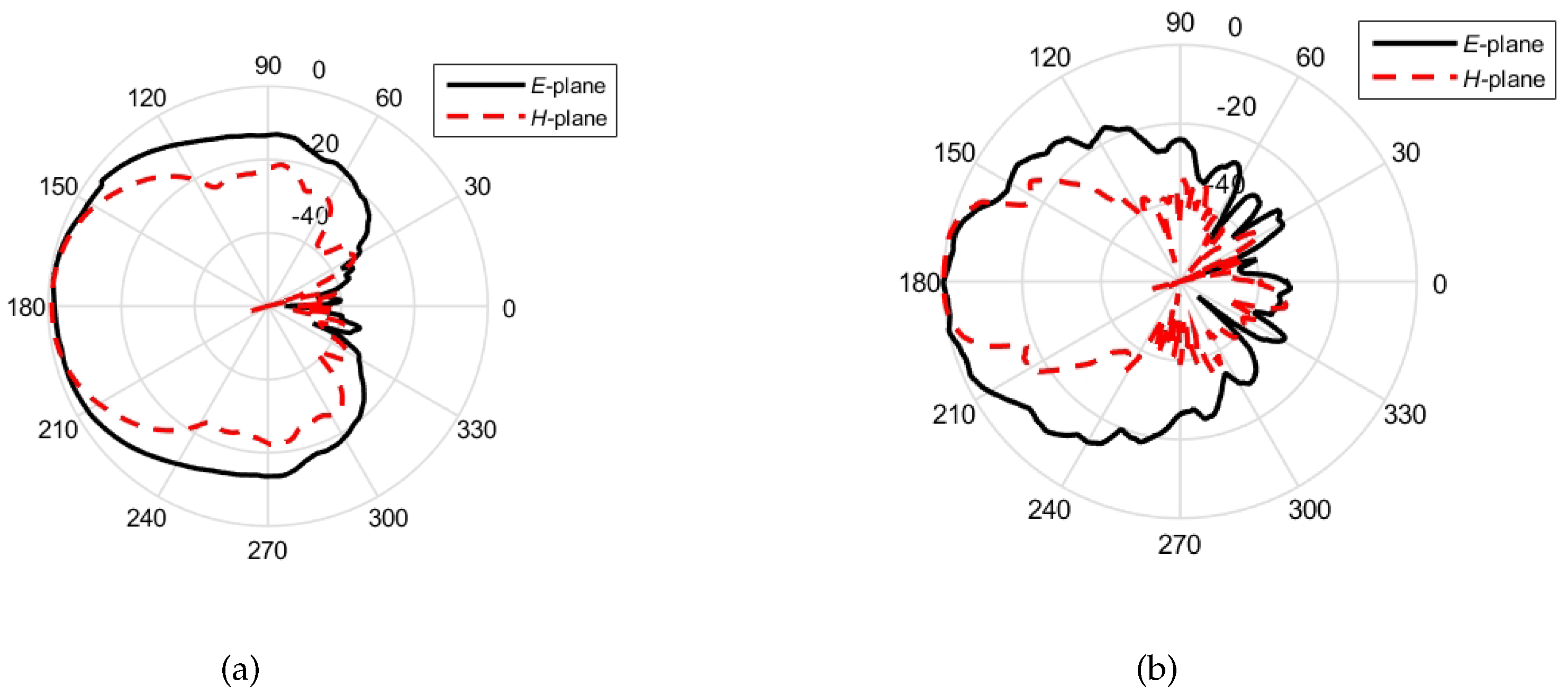
| Beamwidth E-plane | 49 | 43 |
| Beamwidth H-plane | 38 | 34 |
| Gain E-plane | 7 dBi | 12 dBi |
| Gain H-plane | 9 dBi | 14 dBi |
| Sweep Bandwidth | 0.8 GHz | |
| Time Resolution | 1.25 ns | |
| IF Bandwidth | 300 Hz | |
| Acquistion Time (6 sweeps× 900 ms) | 5.4 s | |
| Measured Parameters | 3.6 GHz Band | 14.6 GHz Band | ||
|---|---|---|---|---|
| In the Middle | Near the Wall | In the Middle | Near the Wall | |
| Path Loss Exponent | 1.51 | 1.69 | 1.67 | 1.58 |
| Fit Intercept (dB) | 47.8 | 46.8 | 57.8 | 58.9 |
| Shadow Fading Standard (dB) | 1.79 | 2.19 | 2.27 | 2.16 |
| Mean of RMS Delay Spread (ns) | 12.94 | 13.04 | 14.84 | 13.87 |
| (MHz) | 324.95 | 316.19 | 322.27 | 324.56 |
| (MHz) | 115.92 | 126.29 | 117.42 | 122.60 |
| (MHz) | 37.21 | 42.91 | 43.15 | 42.17 |
| (MHz) | 11.01 | 11.22 | 12.05 | 11.70 |
| (MHz) | 5.21 | 6.07 | 5.16 | 5.78 |
| (MHz) | 1.52 | 1.62 | 1.77 | 1.40 |
| Measured Parameters | Slope | |
|---|---|---|
| 3 Absorbers | 4 Absorbers | |
| RMS delay spread, 1000 MHz (ns/MHz) | ||
| RMS delay spread, 200 MHz (ns/MHz) | ||
| Coherence bandwidth, = 0.5 | ||
| Coherence bandwidth, = 0.7 | ||
| Coherence bandwidth, = 0.9 | ||
© 2017 by the authors. Licensee MDPI, Basel, Switzerland. This article is an open access article distributed under the terms and conditions of the Creative Commons Attribution (CC BY) license ( http://creativecommons.org/licenses/by/4.0/).
Share and Cite
Zhou, X.; Zhong, Z.; Bian, X.; He, R.; Sun, R.; Guan, K.; Liu, K.; Guo, X. Measurement and Analysis of Channel Characteristics in Reflective Environments at 3.6 GHz and 14.6 GHz. Appl. Sci. 2017, 7, 165. https://doi.org/10.3390/app7020165
Zhou X, Zhong Z, Bian X, He R, Sun R, Guan K, Liu K, Guo X. Measurement and Analysis of Channel Characteristics in Reflective Environments at 3.6 GHz and 14.6 GHz. Applied Sciences. 2017; 7(2):165. https://doi.org/10.3390/app7020165
Chicago/Turabian StyleZhou, Xin, Zhangdui Zhong, Xin Bian, Ruisi He, Ruoyu Sun, Ke Guan, Ke Liu, and Xiaotao Guo. 2017. "Measurement and Analysis of Channel Characteristics in Reflective Environments at 3.6 GHz and 14.6 GHz" Applied Sciences 7, no. 2: 165. https://doi.org/10.3390/app7020165
APA StyleZhou, X., Zhong, Z., Bian, X., He, R., Sun, R., Guan, K., Liu, K., & Guo, X. (2017). Measurement and Analysis of Channel Characteristics in Reflective Environments at 3.6 GHz and 14.6 GHz. Applied Sciences, 7(2), 165. https://doi.org/10.3390/app7020165