Machine Learning for Identifying Demand Patterns of Home Energy Management Systems with Dynamic Electricity Pricing

Abstract
1. Introduction
2. Design of Natural Experiment
3. Results
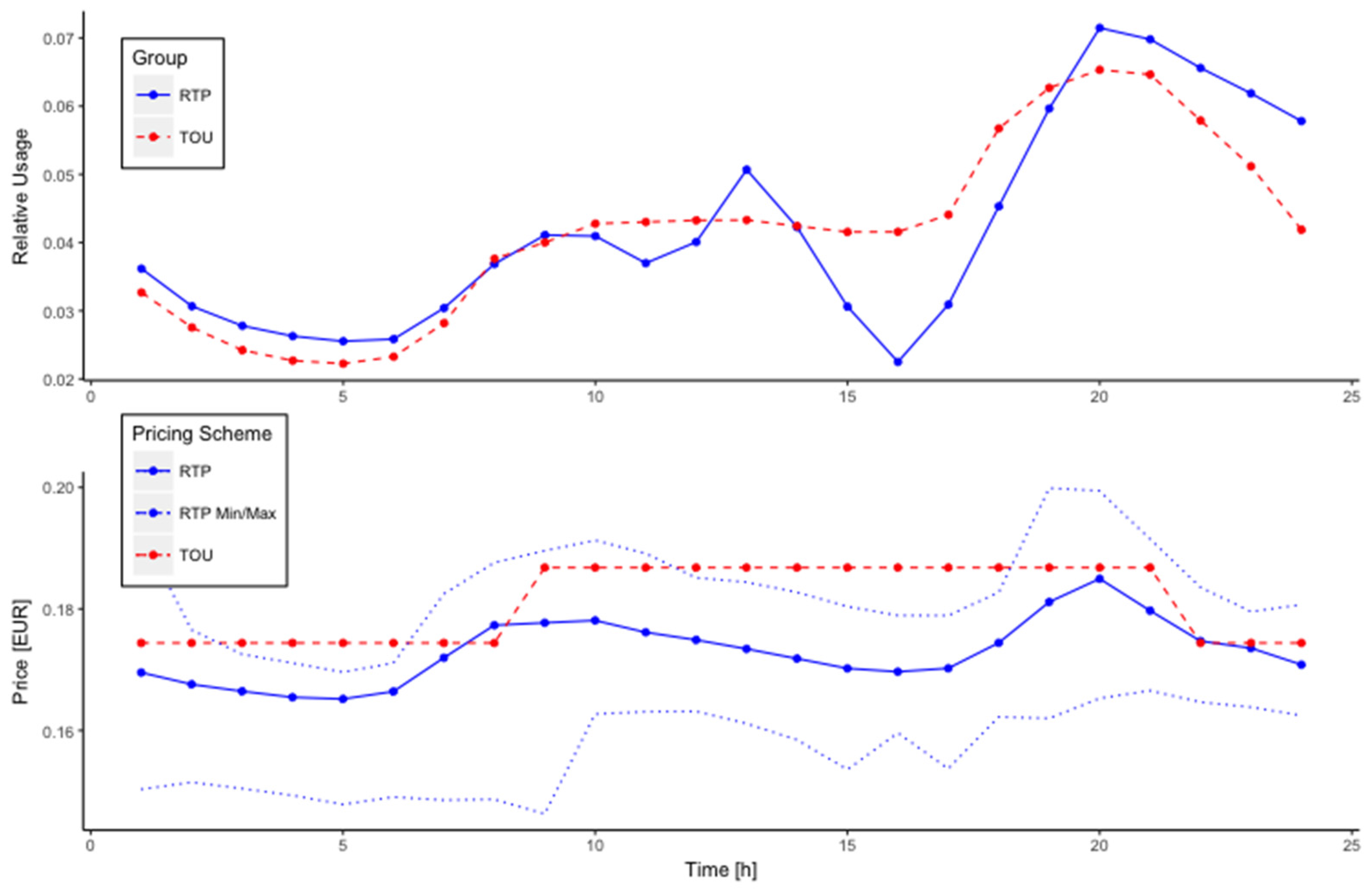
3.1. Panel Data Analysis of Dynamic Pricing Schemes
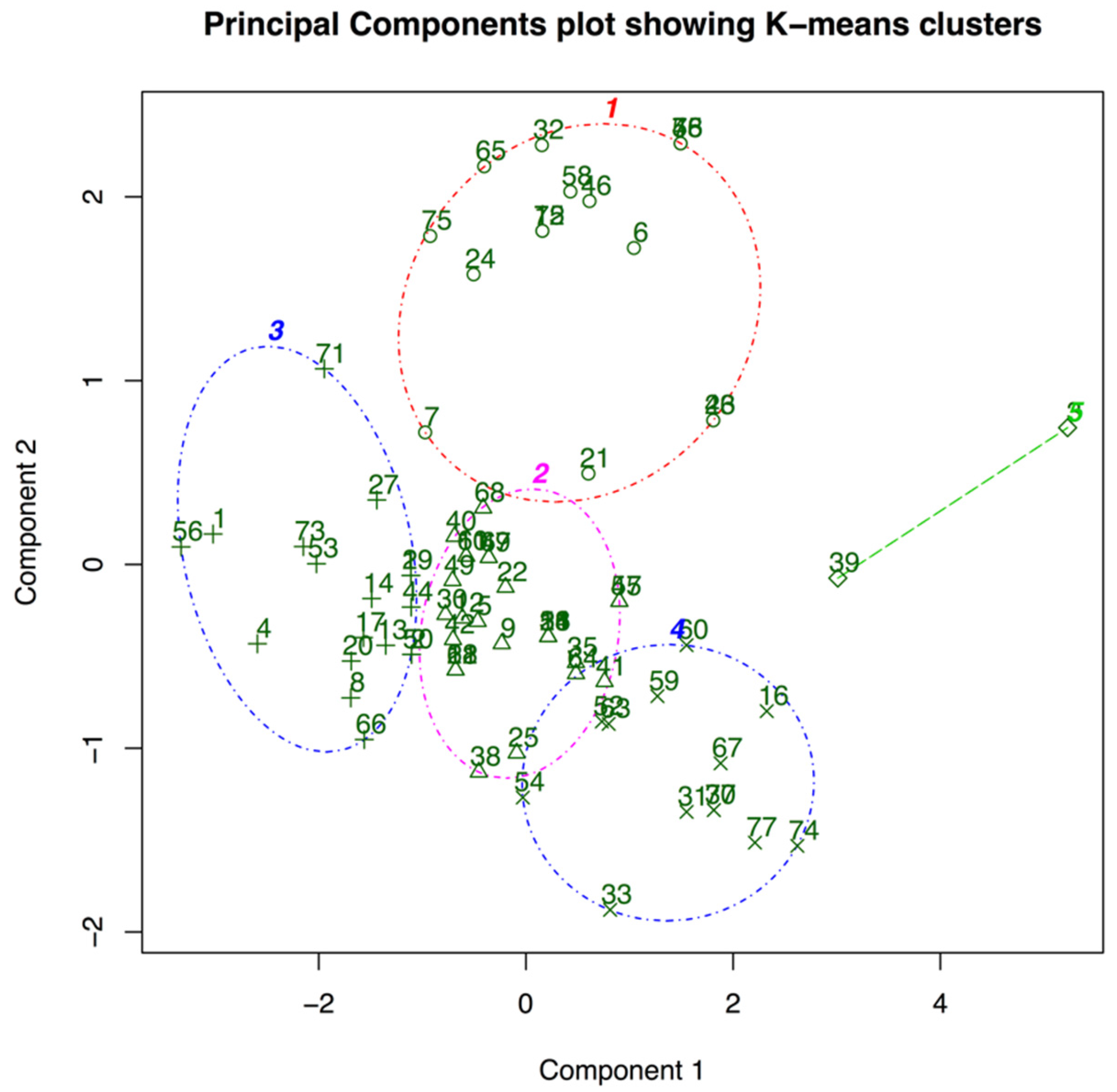
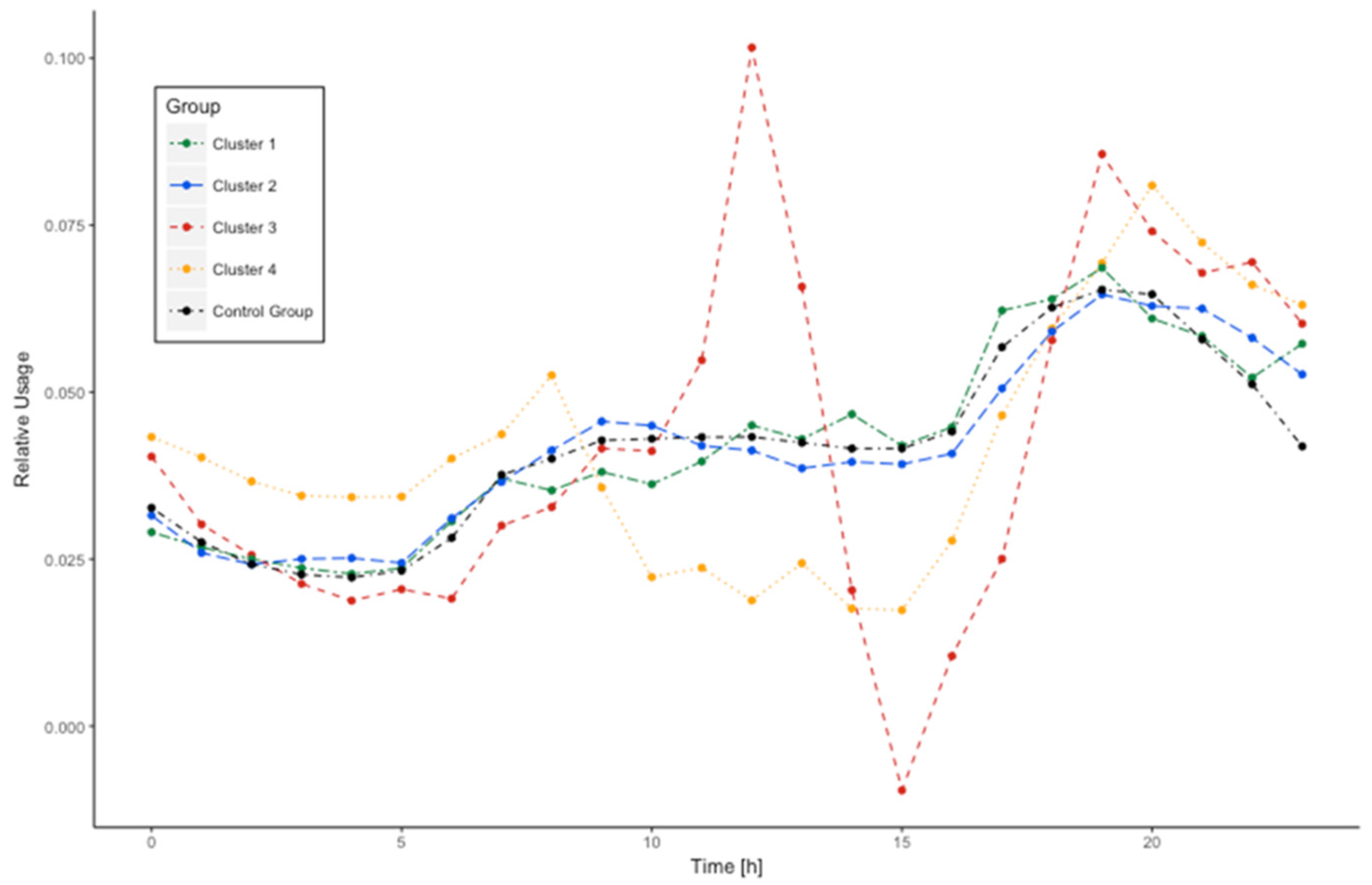
3.2. Reduced Dimension Clustering to Identify Demand Patterns
- ‘Cluster 1’ (18.09) represents 17% of the participating households. The group of households consists of large groups of people, that are only residing in urban or suburban areas. The majority of this group resides in semi-detached and row-houses. The group represents higher-end urban workers with families.
- ‘Cluster 2’ (15.75) represents the largest group of households with 36%. This group represents households living in urban areas, in row or semi-detached houses. The group represents lower-end urban workers.
- ‘Cluster 3’ (14.07) represents 21% of the participating households. The cluster primarily contains three-person households, which live mostly in detached houses, in the city or rural areas. We identify young starters to be present in this group.
- ‘Cluster 4’ (4.59) is characterized by a small group composition of 2 persons on average. They are represented in all classes of building type and terrain, but with a relatively large size of building. We find this group to consist of mainly seniors.
- ‘Cluster 5’ (31.81) is only comprised of 2 households, relatively small in number of occupants, living in detached houses. As the cluster is not found to be significant, it will be ignored for the following elaborations.
4. Conclusions
Acknowledgment
Author Contributions
Conflicts of Interest
Appendix A

| Term | Abreviation | Description |
|---|---|---|
| APX Energy Market | APX | The Dutch spot wholesale electricity market. |
| Real-Time Price | RTP | Type of dynamic pricing tariff, in which customers are informed about, mostly hourly changing, varying electricity prices on a day-ahead or hour-ahead basis [11]. |
| Time-of-Use Price | TOU | Type of Dynamic Pricing, in which prices are changing during specific time periods at a fixed rate. |
| Energy Management System | EMS | Hardware system in households that enables monitoring of energy usage and communication between utility providers and households. |
| Demand-Side Management | DSM | Demand side management strategies, such as demand response, aim to engage consumers of electrical energy, in order to enhance demand flexibility. |
| Demand Response | DR | Demand Response (DR) programs offer financial incentives to take actions to reduce or shift load in correspondence to market price behavior. |
| Incentive-Based Program | IBP | In IBP programs, consumers are offered non-monetary incentives to alter their electricity consumption behavior. |
| Price-Based Program | PBP | In PBP programs, consumers are offered dynamic pricing rates over time, typically with prices significantly higher during peak-periods than during off-peak periods. |
| Variable | Symbol | Description |
|---|---|---|
| Number of Household Occupants | The number of persons permanently occupying a household. | |
| Building Size | The size of a households’ building in square meters. | |
| Building Age | The building age is taken into consideration as a categorical variable with four general categories: 27 years or younger Between 40 and 28 years Between 50 and 41 years 51 years or older | |
| Building Type | The building type a household is residing in, partitioned into five categories. The values of this categorical variable range from one to five. Apartment (‘Appartement’) Row House (‘Tussenwoning’) Detached House (‘Vrijstaand’) Corner House (‘Hoekwoning’) Semi-detached House (‘Twee onder een kap’) | |
| Terrain Type | Terrain Type is a categorical variable that indicates whether a household is located in an ‘Urban’, ‘Suburban’, or ‘Rural’ area. The categorization benchmark was set as follows: Rural—less than 1000 inhabitants per km2 at household location Suburban—between 1000 and 3000 inhabitants per km2 at household location Urban—more than 3000 inhabitants per km2 at household location | |
| PV Panel Ownership | PV panel ownership is included as a dummy variable, indicating 1 as ownership and 0 as non-ownership. | |
| Ventilation Type | Attributed for by a categorical variable. Houses in our study either have ‘Natural’ or ‘Mechanical’ Ventilation. | |
| Roof Insulation | Availability of roof insulation is included as a dummy variable, indicating 1 as available and 0 as not available. | |
| Solar Heating | Availability of solar heating is included as a dummy variable, indicating 1 as available and 0 as not available. | |
| Solar Influx | Potential PV production amount and sunshine intensity measured as the Solar influx in J/cm2. Solar influx was measured as hourly data from the Ministry of Climatology of the Netherlands (KNMI). Moreover, solar influx information was taken from 20 different weather stations. Each household received the solar influx information from the weather station closest to the household. | |
| Time-of-Use Price (TOU) | The TOU electricity prices are composed of a marginal fee of the electricity provider that reflects the forward price and a risk premium. The TOU electricity price changes between peak- and off-peak times. | |
| Real-Time Price (RTP) | The real-time electricity prices are the APX electricity market prices plus any additional surcharges that are generally applicable to electricity end-users. | |
| Price Sensitivity | Price Sensitivity, calculated as: electricity usage/electricity price. | |
| Relative Electricity Usage | Relative Daily Electricity Usage. |
Appendix B
| Price Sensitivity | ||||||||||||||||||||||||
|---|---|---|---|---|---|---|---|---|---|---|---|---|---|---|---|---|---|---|---|---|---|---|---|---|
| (1) | (2) | (3) | (4) | (5) | (6) | (7) | (8) | (9) | (10) | (11) | (12) | (13) | (14) | (15) | (16) | (17) | (18) | (19) | (20) | (21) | (22) | (23) | (24) | |
| Persons | 0.33 *** | 0.19 *** | 0.16 *** | 0.14 *** | 0.16 *** | 0.28 *** | 0.56 *** | 0.27 *** | 0.16 ** | 0.21 *** | 0.39 *** | 0.57 *** | 0.63 *** | 0.79 *** | 0.70 *** | 0.69 *** | 0.76 *** | 0.81 *** | 0.81 *** | 0.82 *** | 0.71 *** | 0.66 *** | 0.61 *** | 0.39 *** |
| (0.05) | (0.04) | (0.04) | (0.03) | (0.03) | (0.04) | (0.05) | (0.05) | (0.07) | (0.08) | (0.09) | (0.10) | (0.10) | (0.09) | (0.08) | (0.07) | (0.07) | (0.06) | (0.07) | (0.06) | (0.06) | (0.06) | (0.06) | (0.05) | |
| B. Age | −0.15 *** | −0.10 ** | −0.09** | −0.15 *** | −0.15 *** | −0.07 * | 0.14 *** | −0.12 ** | −0.48 *** | −0.59 *** | −0.76 *** | −0.92 *** | −0.94 *** | −0.86 *** | −0.69 *** | −0.54 *** | −0.27 *** | −0.05 | 0.10 | 0.18 *** | 0.15** | 0.08 | 0.01 | −0.03 |
| (0.05) | (0.04) | (0.04) | (0.03) | (0.03) | (0.04) | (0.05) | (0.05) | (0.07) | (0.08) | (0.09) | (0.10) | (0.10) | (0.09) | (0.08) | (0.07) | (0.07) | (0.07) | (0.07) | (0.06) | (0.06) | (0.06) | (0.06) | (0.05) | |
| B. Size | 0.01 *** | 0.01 *** | 0.002 *** | 0.003 *** | 0.003 *** | 0.003 *** | 0.002 *** | 0.001 | 0.001 | −0.001 | −0.001 | −0.003 * | −0.003 * | 0.0001 | 0.002 | 0.003 ** | 0.004 *** | 0.01 *** | 0.01 *** | 0.01 *** | 0.01 *** | 0.01 *** | 0.01 *** | 0.01 *** |
| (0.001) | (0.001) | (0.001) | (0.001) | (0.0005) | (0.001) | (0.001) | (0.001) | (0.001) | (0.001) | (0.002) | (0.002) | (0.002) | (0.002) | (0.001) | (0.001) | (0.001) | (0.001) | (0.001) | (0.001) | (0.001) | (0.001) | (0.001) | (0.001) | |
| B. Type | −0.06 | −0.06 | −0.14 *** | −0.20 *** | −0.16 *** | −0.15 *** | −0.04 | −0.005 | 0.02 | 0.01 | 0.04 | −0.05 | −0.02 | −0.19** | −0.25 *** | −0.31 *** | −0.07 | −0.03 | −0.07 | −0.08 | −0.09 | −0.02 | 0.09 | −0.002 |
| (0.05) | (0.04) | (0.04) | (0.03) | (0.03) | (0.04) | (0.05) | (0.05) | (0.07) | (0.08) | (0.09) | (0.10) | (0.10) | (0.09) | (0.08) | (0.07) | (0.07) | (0.07) | (0.07) | (0.07) | (0.06) | (0.06) | (0.06) | (0.05) | |
| Roof Insul. | −0.18 | −0.13 | 0.01 | 0.16 | 0.19** | 0.24 * | −0.09 | −0.38 ** | −0.53 ** | −0.79 *** | −1.23 *** | −1.20 *** | −1.47 *** | −0.99 *** | −0.95 *** | −0.38 * | 0.16 | 0.40 * | 0.42 * | 0.42 ** | 0.55 *** | 0.27 | −0.31 * | −0.25 |
| (0.16) | (0.14) | (0.12) | (0.10) | (0.09) | (0.13) | (0.17) | (0.17) | (0.23) | (0.26) | (0.30) | (0.32) | (0.32) | (0.30) | (0.25) | (0.22) | (0.22) | (0.21) | (0.22) | (0.21) | (0.20) | (0.20) | (0.19) | (0.16) | |
| SolarInflux | −0.01 ** | −0.01 *** | −0.02 *** | −0.02 *** | −0.02 *** | −0.02 *** | −0.02 *** | −0.02 *** | −0.02 *** | −0.02 *** | −0.05 ** | 0.36 | ||||||||||||
| (0.003) | (0.002) | (0.002) | (0.002) | (0.002) | (0.002) | (0.002) | (0.002) | (0.003) | (0.005) | (0.02) | (0.52) | |||||||||||||
| Constant | 0.44 | 0.53 | 1.51 *** | 1.39 *** | 0.75** | 0.68 | −0.001 | 3.10 *** | 5.38 *** | 7.39 *** | 7.51 *** | 7.89 *** | 8.65 *** | 6.49 *** | 6.06 *** | 3.52 *** | 2.08** | 0.32 | −0.15 | −0.72 | −0.02 | 0.51 | −0.12 | 0.18 |
| (0.51) | (0.46) | (0.39) | (0.34) | (0.31) | (0.42) | (0.58) | (0.60) | (0.81) | (0.94) | (1.04) | (1.09) | (1.13) | (1.08) | (0.92) | (0.79) | (0.81) | (0.84) | (0.73) | (0.69) | (0.65) | (0.65) | (0.60) | (0.56) | |
| Observations | 1990 | 1923 | 1987 | 1991 | 1991 | 1991 | 1990 | 1991 | 1991 | 1991 | 1991 | 1991 | 1991 | 1991 | 1991 | 1991 | 1991 | 1991 | 1991 | 1991 | 1991 | 1991 | 1999 | 2100 |
| R2 | 0.12 | 0.07 | 0.02 | 0.05 | 0.06 | 0.04 | 0.07 | 0.03 | 0.05 | 0.07 | 0.08 | 0.09 | 0.09 | 0.10 | 0.10 | 0.09 | 0.08 | 0.10 | 0.10 | 0.13 | 0.11 | 0.10 | 0.15 | 0.13 |
| Adjusted R2 | 0.12 | 0.07 | 0.02 | 0.05 | 0.06 | 0.04 | 0.07 | 0.03 | 0.05 | 0.06 | 0.08 | 0.09 | 0.09 | 0.10 | 0.10 | 0.09 | 0.08 | 0.10 | 0.10 | 0.13 | 0.11 | 0.10 | 0.15 | 0.13 |
| F Statistic | 44.94 *** (df = 6; 1983) | 23.63 *** (df = 6; 1916) | 7.86 *** (df = 6; 1980) | 17.64 *** (df = 6; 1984) | 21.00 *** (df = 6; 1984) | 15.22 *** (df = 6; 1984) | 25.33 *** (df = 6; 1983) | 7.96 *** (df = 7; 1983) | 14.13 *** (df = 7; 1983) | 19.76 *** (df = 7; 1983) | 25.28 *** (df = 7; 1983) | 27.88 *** (df = 7; 1983) | 28.67 *** (df = 7; 1983) | 29.98 *** (df = 7; 1983) | 31.26 *** (df = 7; 1983) | 29.59 *** (df = 7; 1983) | 25.23 *** (df = 7; 1983) | 32.48 *** (df = 7; 1983) | 30.67 *** (df = 7; 1983) | 49.79 *** (df = 6; 1984) | 42.30 *** (df = 6; 1984) | 35.68 *** (df = 6; 1984) | 60.02 *** (df = 6; 1992) | 51.44 *** (df = 6; 2093) |
Appendix C
| Price Sensitivity | ||||||||||||||||||||||||
|---|---|---|---|---|---|---|---|---|---|---|---|---|---|---|---|---|---|---|---|---|---|---|---|---|
| (1) | (2) | (3) | (4) | (5) | (6) | (7) | (8) | (9) | (10) | (11) | (12) | (13) | (14) | (15) | (16) | (17) | (18) | (19) | (20) | (21) | (22) | (23) | (24) | |
| Persons | −0.15 | −0.08 | −0.14 | −0.19* | −0.15 | −0.10 | 0.14 ** | 0.13 | 0.21 ** | 0.23 * | 0.41 *** | 0.37 *** | 0.39 *** | 0.26 ** | 0.20 | 0.41 *** | 0.54 *** | 0.52 *** | 0.54 *** | 0.59 *** | 0.27 ** | 0.15 | −0.09 | −0.19 |
| (0.11) | (0.09) | (0.10) | (0.11) | (0.10) | (0.07) | (0.07) | (0.08) | (0.10) | (0.12) | (0.11) | (0.11) | (0.11) | (0.12) | (0.12) | (0.11) | (0.12) | (0.11) | (0.15) | (0.15) | (0.11) | (0.09) | (0.12) | (0.13) | |
| B. Age | 0.13 | 0.01 | 0.01 | 0.06 | 0.06 | 0.05 | −0.09 | −0.08 | −0.10 | −0.06 | −0.17 | −0.10 | −0.11 | 0.04 | 0.02 | −0.02 | −0.22* | −0.36 *** | −0.15 | −0.06 | −0.15 | −0.22 ** | −0.03 | 0.14 |
| (0.10) | (0.08) | (0.09) | (0.10) | (0.09) | (0.07) | (0.06) | (0.08) | (0.10) | (0.11) | (0.11) | (0.10) | (0.10) | (0.11) | (0.11) | (0.10) | (0.11) | (0.10) | (0.14) | (0.14) | (0.11) | (0.09) | (0.11) | (0.12) | |
| B. Size | 0.02 *** | 0.02 *** | 0.02 *** | 0.02 *** | 0.02 *** | 0.02 *** | 0.02 *** | 0.02 *** | 0.02 *** | 0.03 *** | 0.02 *** | 0.02 *** | 0.02 *** | 0.02 *** | 0.02 *** | 0.02 *** | 0.02 *** | 0.02 *** | 0.01 *** | 0.02 *** | 0.02 *** | 0.02 *** | 0.02 *** | 0.02 *** |
| (0.001) | (0.001) | (0.001) | (0.001) | (0.001) | (0.001) | (0.001) | (0.001) | (0.001) | (0.001) | (0.001) | (0.001) | (0.001) | (0.001) | (0.001) | (0.001) | (0.001) | (0.001) | (0.002) | (0.002) | (0.001) | (0.001) | (0.001) | (0.001) | |
| B. Type | 0.18 ** | 0.07 | 0.08 | 0.11 | 0.16 ** | 0.12 ** | 0.14 ** | 0.23 *** | 0.16* | 0.17* | 0.19** | 0.15* | 0.19** | 0.27 *** | 0.24** | 0.23 *** | 0.17* | 0.28 *** | 0.44 *** | 0.38 *** | 0.33 *** | 0.18 ** | 0.22 ** | 0.22 ** |
| (0.09) | (0.07) | (0.08) | (0.09) | (0.08) | (0.06) | (0.05) | (0.07) | (0.09) | (0.09) | (0.09) | (0.09) | (0.09) | (0.10) | (0.10) | (0.09) | (0.10) | (0.09) | (0.12) | (0.12) | (0.09) | (0.08) | (0.10) | (0.10) | |
| Roof Insul. | −0.16 | −0.18 | −0.16 | −0.14 | −0.35 | −0.60 *** | −0.45 ** | −0.75 *** | −0.98 *** | −1.02 *** | −1.09 *** | −0.96 *** | −0.99 *** | −1.22 *** | −1.15 *** | −1.32 *** | −0.29 | 0.28 | 0.12 | 0.22 | 0.06 | 0.19 | −0.08 | −0.12 |
| (0.29) | (0.24) | (0.26) | (0.30) | (0.26) | (0.19) | (0.18) | (0.23) | (0.28) | (0.32) | (0.31) | (0.29) | (0.30) | (0.33) | (0.33) | (0.30) | (0.32) | (0.30) | (0.40) | (0.39) | (0.31) | (0.25) | (0.32) | (0.34) | |
| SolarInflux | −0.001 | −0.001 | −0.001 | −0.002 | −0.002 | −0.001 | −0.002 | 0.0000 | −0.003 | −0.01 | −0.03 | 0.09 | ||||||||||||
| (0.004) | (0.002) | (0.002) | (0.002) | (0.001) | (0.002) | (0.002) | (0.003) | (0.004) | (0.01) | (0.02) | (0.34) | |||||||||||||
| Constant | −1.16 | −1.33 * | −1.71 ** | −2.08 ** | −1.40 ** | −0.96 * | −0.70 | −0.46 | 1.04 | 0.58 | 0.74 | 1.11 | 1.15 | 1.93 | 1.91 | 1.01 | 0.13 | −1.06 | −2.82 *** | −2.55 ** | 0.66 | 0.31 | −0.43 | −0.85 |
| (0.87) | (0.76) | (0.79) | (0.90) | (0.71) | (0.55) | (0.64) | (0.75) | (0.87) | (0.90) | (0.93) | (0.86) | (0.95) | (1.19) | (1.24) | (1.09) | (1.00) | (1.08) | (1.04) | (1.10) | (0.97) | (0.84) | (1.06) | (1.03) | |
| Observations | 1020 | 986 | 1020 | 1020 | 1020 | 1020 | 1020 | 1020 | 1020 | 1020 | 1020 | 1020 | 1020 | 1020 | 1020 | 1020 | 1020 | 1020 | 1020 | 1020 | 1020 | 1020 | 1020 | 1020 |
| R2 | 0.18 | 0.26 | 0.24 | 0.19 | 0.20 | 0.37 | 0.46 | 0.41 | 0.32 | 0.31 | 0.31 | 0.30 | 0.33 | 0.28 | 0.26 | 0.27 | 0.25 | 0.22 | 0.14 | 0.16 | 0.20 | 0.22 | 0.16 | 0.14 |
| Adjusted R2 | 0.18 | 0.25 | 0.24 | 0.19 | 0.20 | 0.37 | 0.46 | 0.41 | 0.32 | 0.31 | 0.31 | 0.30 | 0.33 | 0.28 | 0.26 | 0.26 | 0.25 | 0.22 | 0.13 | 0.16 | 0.19 | 0.21 | 0.16 | 0.14 |
| F Statistic | 38.18 *** (df = 6; 1013) | 56.04 *** (df = 6; 979) | 53.64 *** (df = 6; 1013) | 39.62 *** (df = 6; 1013) | 42.25 *** (df = 6; 1013) | 99.79 *** (df = 6; 1013) | 143.90 *** (df = 6; 1013) | 99.79 *** (df = 7; 1012) | 69.06 *** (df = 7; 1012) | 64.72 *** (df = 7; 1012) | 65.55 *** (df = 7; 1012) | 61.76 *** (df = 7; 1012) | 70.83 *** (df = 7; 1012) | 55.69 *** (df = 7; 1012) | 51.40 *** (df = 7; 1012) | 52.34 *** (df = 7; 1012) | 49.13 *** (df = 7; 1012) | 41.90 *** (df = 7; 1012) | 22.66 *** (df = 7; 1012) | 31.83 *** (df = 6; 1013) | 41.12 *** (df = 6; 1013) | 46.45 *** (df = 6; 1013) | 32.78 *** (df = 6; 1013) | 28.13 *** (df = 6; 1013) |
References
- Ketter, W.; Peters, M.; Collins, J.; Gupta, A. A Multiagent Competitive Gaming Platform to Address Societal Challenges. MIS Q. 2016, 40, 447–460. [Google Scholar] [CrossRef]
- Osório, G.J.; Gonçalves, J.N.; Lujano-Rojas, J.M.; Catalão, J.P. Enhanced forecasting approach for electricity market prices and wind power data series in the short-term. Energies 2016, 9, 693. [Google Scholar] [CrossRef]
- Bichler, M.; Gupta, A.; Ketter, W. Designing smart markets. Inf. Syst. Res. 2010, 21, 688–699. [Google Scholar] [CrossRef]
- Conejo, A.J.; Morales, J.M.; Baringo, L. Real-time demand response model. IEEE Trans. Smart Grid 2010, 1, 236–242. [Google Scholar] [CrossRef]
- Yener, B.; Taşcıkaraoğlu, A.; Erdinç, O.; Baysal, M.; Catalão, J.P. Design and Implementation of an Interactive Interface for Demand Response and Home Energy Management Applications. Appl. Sci. 2017, 7, 641. [Google Scholar] [CrossRef]
- Vahedipour-Dahraie, M.; Najafi, H.R.; Anvari-Moghaddam, A.; Guerrero, J.M. Study of the Effect of Time-Based Rate Demand Response Programs on Stochastic Day-Ahead Energy and Reserve Scheduling in Islanded Residential Microgrids. Appl. Sci. 2017, 7, 378. [Google Scholar] [CrossRef]
- Pina, A.; Silva, C.; Ferrao, P. The impact of demand side management strategies in the penetration of renewable electricity. Energy 2012, 41, 128–137. [Google Scholar] [CrossRef]
- Torriti, J.; Hassen, M.; Leach, M. Demand response experience in Europe: Policies, prgrammes and implementation. Energy 2010, 35, 1575–1583. [Google Scholar] [CrossRef]
- Albadi, M.; El-Saadany, E. Demand Response in Electricity Markets: An Overview. Power Eng. Soc. Gen. Meet. 2007, 1–5. [Google Scholar] [CrossRef]
- Palensky, P.; Dietrich, D. Demand Side Management: Demand Response, Intelligent Energy Systems, and Smart Loads. IEEE Trans. Ind. Inf. 2011, 7, 381–388. [Google Scholar] [CrossRef]
- Contreras, J.; Asensio, M.; Meneses de Quevedo, P.; Munoz-Delgado, G.; Montaya-Bueno, S. Joint RES and Distribution Network Expansion Planning under A Demand Response Framework, 1st ed.; Academic Press: London, UK, 2016; ISBN 9780128053225. [Google Scholar]
- Fischer, C. Feedback on Household Electricity Consumption: A Tool for Saving Energy? Energy Effic. 2008, 1, 79–104. [Google Scholar] [CrossRef]
- Borenstein, S.; Jaske, M.; Ros, A. Dynamic Pricing, Advanced Metering, and Demand Response in Electricity Markets. J. Am. Chem. Soc. 2002, 128, 4136–4145. [Google Scholar]
- Ketter, W.; Collins, J.; Reddy, P. Power TAC: A competitive economic simulation of the smart grid. Energy Econ. 2013, 39, 262–270. [Google Scholar] [CrossRef]
- Alcott, H. Rethinking real-time electricity pricing. Resour. Energy Econ. 2011, 33, 820–842. [Google Scholar] [CrossRef]
- Bartush, C.; Wallin, F.; Odlare, M. Introducing a demand-based electricity distribution tariff in the residential sector: Demand response and customer perception. Energy Policy 2011, 39, 5008–5025. [Google Scholar] [CrossRef]
- Gottwalt, S.; Ketter, W.; Block, C.; Collins, J.; Weinhardt, C. Demand side management—A simulation of household behavior under variable prices. Energy Policy 2011, 39, 8163–8174. [Google Scholar] [CrossRef]
- Nababan, T. Analysis of Household Characteristics Affecting the Demand of PLN’s Electricity. An Observation on Small Households in City of Medan, Indonesia. Acad. J. Econ. Stud. 2015, 1, 79–92. [Google Scholar]
- Di Cosmo, V.; Lyons, S.; Nolan, A. Estimating the impact of time-of-use pricing on Irish electricity demand. Energy J. 2014, 35, 1–26. [Google Scholar] [CrossRef]
- Wilhite, H.; Ling, R. Measured Energy Savings from a More Informative Energy Bill. Energy Build. 1995, 22, 145–155. [Google Scholar] [CrossRef]
- Vine, D.; Buys, L. The Effectiveness of Energy Feedback for Conservation and Peak Demand: A Literature Review. Open J. Energy Effic. 2013, 2, 7–15. [Google Scholar] [CrossRef]
- Brandon, G.; Lewis, A. Reducing Household Energy Consumption: A Qualitative and Quantitative Field Study. J. Environ. Psychol. 1999, 19, 75–85. [Google Scholar] [CrossRef]
- Schleich, J.; Klobasa, M. How much shift in demand? Findings from a field experiment in Germany. In Proceedings of the ECEEE 2013 Summer Study–Rethink, Renew, Restart, Saint-Raphaël, France, 2–7 June 2013; Volume 1, pp. 1919–1925. [Google Scholar]
- Yohannis, Y.; Mondol, J.; Wright, A.; Norton, B. Real-Life energy use in the UK: How occupancy and dwelling characteristics affect domestic electricity use. Energy Build. 2008, 40, 1053–1059. [Google Scholar] [CrossRef]
- McLoughlin, F.; Duffy, A.; Conlon, M. Characterising Domestic electricity consumption patterns by dwelling and occupant socio-economic variables: An Irish case study. Energy Build. 2012, 48, 240–248. [Google Scholar] [CrossRef]
- Kavousian, A.; Rajagopal, R.; Fischer, M. Determinants of residential electricity consumption: Using smart meter data to examine the effect of climate, building characteristics, appliance stock, and occupants’ behavior. Energy 2013, 55, 184–194. [Google Scholar] [CrossRef]
- Filippini, M. Short-and long-run time-of-use price elasticities in Swiss residential electricity demand. Energy Policy 2011, 39, 5811–5817. [Google Scholar] [CrossRef]
- Alberini, A.; Gans, W.; Velez-Lopez, D. Residential consumption of gas and electricity in the US: The role of prices and income. Energy Econ. 2011, 33, 870–881. [Google Scholar] [CrossRef]
- Zhou, K.; Fu, C.; Yang, S. Big data driven smart energy management: From big data to big insights. Renew. Sustain. Energy Rev. 2016, 56, 215–225. [Google Scholar] [CrossRef]
- Ding, C.; Li, T. Adaptive dimension reduction using discriminant analysis and k-means clustering. In Proceedings of the 24th International Conference on Machine Learning, New York, NY, USA, 20–24 June 2007; pp. 521–528. [Google Scholar]
- Ye, J.; Zhao, Z.; Wu, M. Discriminative k-means for clustering. In Proceedings of the 20th International Conference on Neural Information Processing Systems (NIPS 2007), Vancouver, BC, Canada, 3–6 December 2007; Curran Associates Inc.: Red Hook, NY, USA, 2007; pp. 1649–1656. [Google Scholar]
- Alzate, C.; Sinn, M. Improved electricity load forecasting via kernel spectral clustering of smart meters. In Proceedings of the 2013 IEEE 13th International Conference on Data Mining (ICDM), Dallas, TX, USA, 4–7 December 2013; pp. 943–948. [Google Scholar]
- Abreu, J.M.; Pereira, F.C.; Ferrão, P. Using pattern recognition to identify habitual behavior in residential electricity consumption. Energy Build. 2012, 49, 479–487. [Google Scholar] [CrossRef]
- Eurelectric. Dynamic pricing in electricity supply. In Eurelectric Position Paper; Eurelectric: Brussels, Belgium, 2017. [Google Scholar]
- Koolen, D.; Ketter, W.; Qiu, L.; Alok, G. The sustainability tipping point in electricity markets. In Proceedings of the 2017 International Conference on Information Systems, Seoul, Korea, 10–13 December 2017. in press. [Google Scholar]
- The APX Power Spot Exchange. Available online: http://www.apxgroup.com/apx-power-nl/ (accessed on 8 July 2016).
- Baltagi, B. Econometric Analysis of Panel Data, 5th ed.; John Wiley & Sons: Hoboken, NJ, USA, 2013; ISBN 978-1118672327. [Google Scholar]
- Greene, W. Econometric Analysis, 5th ed.; New Pearson Education: Hoboken, NJ, USA, 2008; ISBN 978-0130661890. [Google Scholar]
- Yang, S.L.; Shen, C. A review of electric load classification in smart grid environment. Renew. Sustain. Energy Rev. 2013, 24, 103–110. [Google Scholar]
- Ferreira, A.M.; Cavalcante, C.A.; Fontes, C.H.; Marambio, J.E. A new method for pattern recognition in load profiles to support decision-making in the management of the electric sector. Int. J. Electr. Power Energy Syst. 2013, 53, 824–831. [Google Scholar] [CrossRef]
- Räsänen, T.; Voukantsis, D.; Niska, H.; Karatzas, K.; Kolehmainen, M. Data-based method for creating electricity use load profiles using large amount of customer-specific hourly measured electricity use data. Appl. Energy 2010, 87, 3538–3545. [Google Scholar] [CrossRef]
- Zhou, K.L.; Yang, S.L. An improved fuzzy C-means algorithm for power load characteristics classification. Power Syst. Prot. Control 2012, 40, 58–63. [Google Scholar]
- Liu, L.; Wang, G.; Zhai, D.H. Application of k-means clustering algorithm in load curve classification. Power Syst. Prot. Control 2011, 39, 65–68. [Google Scholar]
- Mahmoudi-Kohan, N.; Moghaddam, M.P.; Sheikh-El-Eslami, M.K. An annual framework for clustering-based pricing for an electricity retailer. Electr. Power Syst. Res. 2010, 80, 1042–1048. [Google Scholar] [CrossRef]
- Zha, H.; He, X.; Ding, C.; Gu, M.; Simon, H.D. Spectral relaxation for k-means clustering. In Advances in Neural Information Processing Systems; The MIT Press: Cambridge, MA, USA, 2002; pp. 1057–1064. [Google Scholar]
- Napoleon, D.; Pavalakodi, S. A new method for dimensionality reduction using k-means clustering algorithm for high dimensional data set. Int. J. Comput. Appl. 2011, 13, 41–46. [Google Scholar]


| Author | Number of Household Occupants | Building Size | Building Age | Building Type | Other Attributes | |
|---|---|---|---|---|---|---|
| Schleich and Klobasa (2013) | + | + | No. Appliances | |||
| Yohannis et al. (2008) | + | + | + | + | No. Bedrooms | |
| McLoughlin et al. (2012) | + | + | + | + | Composition | |
| Kavousian et al. (2013) | + | + | insignificant | insignificant | ||
| Filippini (2011) | insignificant | + | Income | |||
| Alberini et al. (2011) | insignificant | + |
| Attributes | Mean | Median | Min | Max | ||||
|---|---|---|---|---|---|---|---|---|
| Solar Influx | 37.74 | 1 | 0 | 259 | ||||
| RTP | TOU | |||||||
| Mean | Median | Min | Max | Mean | Median | Min | Max | |
| Persons | 2.63 | 2 | 1 | 6 | 2.967 | 3 | 1 | 8 |
| Building Age | 2.739 | 3 | 1 | 4 | 2.239 | 2 | 1 | 4 |
| Building Size | 158.2 | 140 | 58 | 550 | 153.5 | 123 | 50 | 600 |
| Building Type | 3.416 | 3 | 1 | 5 | 3.02 | 3 | 1 | 5 |
| Heating Type | 1.185 | 2 | 1 | 2 | 1.219 | 2 | 1 | 2 |
| Roof Insulation | 1.853 | 2 | 1 | 2 | 1.76 | 2 | 1 | 2 |
| Relative Electricity Usage | ||
|---|---|---|
| Treatment | RTP | TOU |
| 0.78 *** | ||
| (0.28) | ||
| 0.95 *** | ||
| (0.04) | ||
| Solar Influx | −0.0002 *** | −0.0000 *** |
| (0.0000) | (0.0000) | |
| Constant | −0.10 ** | −0.13 *** |
| (0.05) | (0.01) | |
| Observations N R2 | 47,275 73 0.34 | 103,515 150 0.48 |
| Adjusted R2 | 0.34 | 0.48 |
| Price Sensitivity | |
|---|---|
| Number of Household Occupants | 0.18 *** |
| (0.02) | |
| Building Age | 0.06 *** |
| (0.02) | |
| Building Size | 0.02 *** |
| (0.0003) | |
| Building Type | 0.20 *** |
| (0.02) | |
| Roof Insulation | −0.47 |
| (0.06) | |
| RTP * Number of Household Occupants | 0.33 *** |
| (0.03) | |
| RTP * Building Age | −0.22 *** |
| (0.03) | |
| RTP * Building Size | −0.02 *** |
| (0.0004) | |
| RTP * Building Type | −0.25 *** |
| (0.02) | |
| RTP * Roof Insulation | 0.29 |
| (0.08) | |
| Solar Influx | −0.01 *** |
| (0.0002) | |
| Constant | 2.08 *** |
| (0.25) | |
| Observations | 72,273 |
| N R2 | 108 0.13 |
| Adjusted R2 | 0.13 |
| F Statistic | 803.61 *** (df = 12; 72,259) |
| PC1 | PC2 | PC3 | PC4 | PC5 | PC6 | PC7 | PC8 | PC9 | |
|---|---|---|---|---|---|---|---|---|---|
| Standard deviation | 1.74 | 1.22 | 1.10 | 1.00 | 0.96 | 0.84 | 0.63 | 0.51 | 0.00 |
| Proportion of Variance | 0.33 | 0.17 | 0.13 | 0.11 | 0.10 | 0.08 | 0.04 | 0.03 | 0.00 |
| Cumulative Proportion | 0.33 | 0.50 | 0.64 | 0.75 | 0.85 | 0.93 | 0.97 | 1.00 | 1.00 |
| Building Age | 0.29 | −0.19 | −0.43 | −0.17 | −0.47 | −0.53 | 0.27 | −0.04 | 0.29 |
| Building Size | −0.56 | 0.15 | 0.05 | 0.09 | −0.07 | 0.01 | −0.12 | −0.06 | 0.79 |
| Building Type | 0.28 | −0.53 | 0.11 | 0.25 | 0.43 | 0.23 | 0.39 | −0.21 | 0.38 |
| Solar Panels | −0.03 | −0.24 | 0.37 | −0.80 | 0.25 | −0.24 | −0.18 | −0.09 | 0.10 |
| Terrain Type | 0.45 | −0.04 | −0.04 | 0.29 | 0.16 | −0.22 | −0.77 | −0.04 | 0.20 |
| Persons | 0.42 | 0.39 | 0.04 | −0.22 | 0.15 | 0.19 | −0.22 | −0.68 | 0.24 |
| Solar Heating | −0.04 | −0.05 | −0.73 | −0.35 | 0.17 | 0.49 | −0.21 | −0.14 | 0.05 |
| Ventilation Type | 0.27 | 0.15 | 0.09 | −0.06 | 0.08 | −0.01 | 0.12 | −0.67 | 0.14 |
| Roof Insulation | 0.25 | −0.16 | 0.33 | −0.11 | −0.67 | 0.54 | −0.18 | −0.10 | 0.11 |
© 2017 by the authors. Licensee MDPI, Basel, Switzerland. This article is an open access article distributed under the terms and conditions of the Creative Commons Attribution (CC BY) license (http://creativecommons.org/licenses/by/4.0/).
Share and Cite
Koolen, D.; Sadat-Razavi, N.; Ketter, W. Machine Learning for Identifying Demand Patterns of Home Energy Management Systems with Dynamic Electricity Pricing. Appl. Sci. 2017, 7, 1160. https://doi.org/10.3390/app7111160
Koolen D, Sadat-Razavi N, Ketter W. Machine Learning for Identifying Demand Patterns of Home Energy Management Systems with Dynamic Electricity Pricing. Applied Sciences. 2017; 7(11):1160. https://doi.org/10.3390/app7111160
Chicago/Turabian StyleKoolen, Derck, Navid Sadat-Razavi, and Wolfgang Ketter. 2017. "Machine Learning for Identifying Demand Patterns of Home Energy Management Systems with Dynamic Electricity Pricing" Applied Sciences 7, no. 11: 1160. https://doi.org/10.3390/app7111160
APA StyleKoolen, D., Sadat-Razavi, N., & Ketter, W. (2017). Machine Learning for Identifying Demand Patterns of Home Energy Management Systems with Dynamic Electricity Pricing. Applied Sciences, 7(11), 1160. https://doi.org/10.3390/app7111160