Albatross-Like Utilization of Wind Gradient for Unpowered Flight of Fixed-Wing Aircraft


Abstract
:1. Introduction
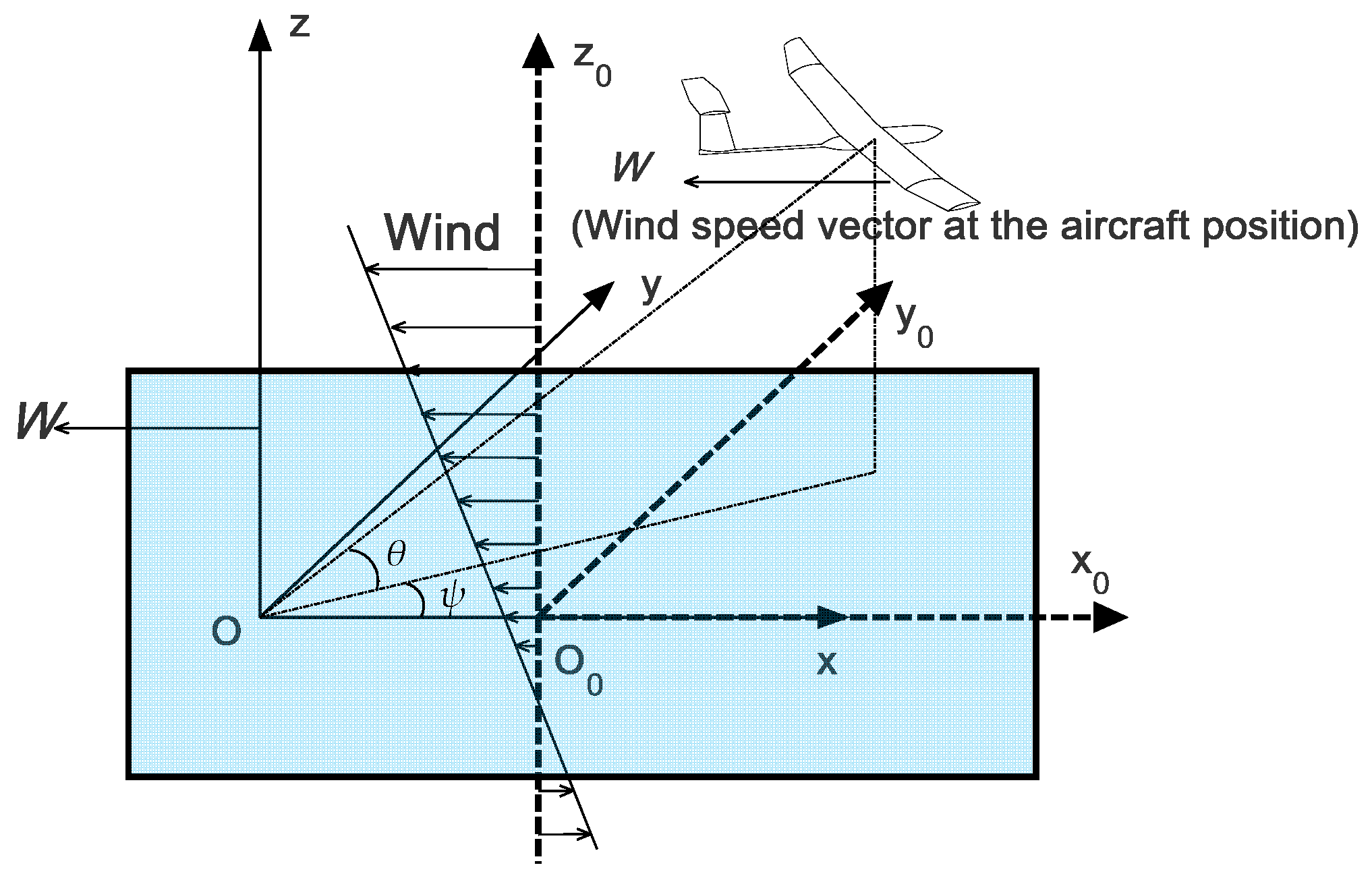
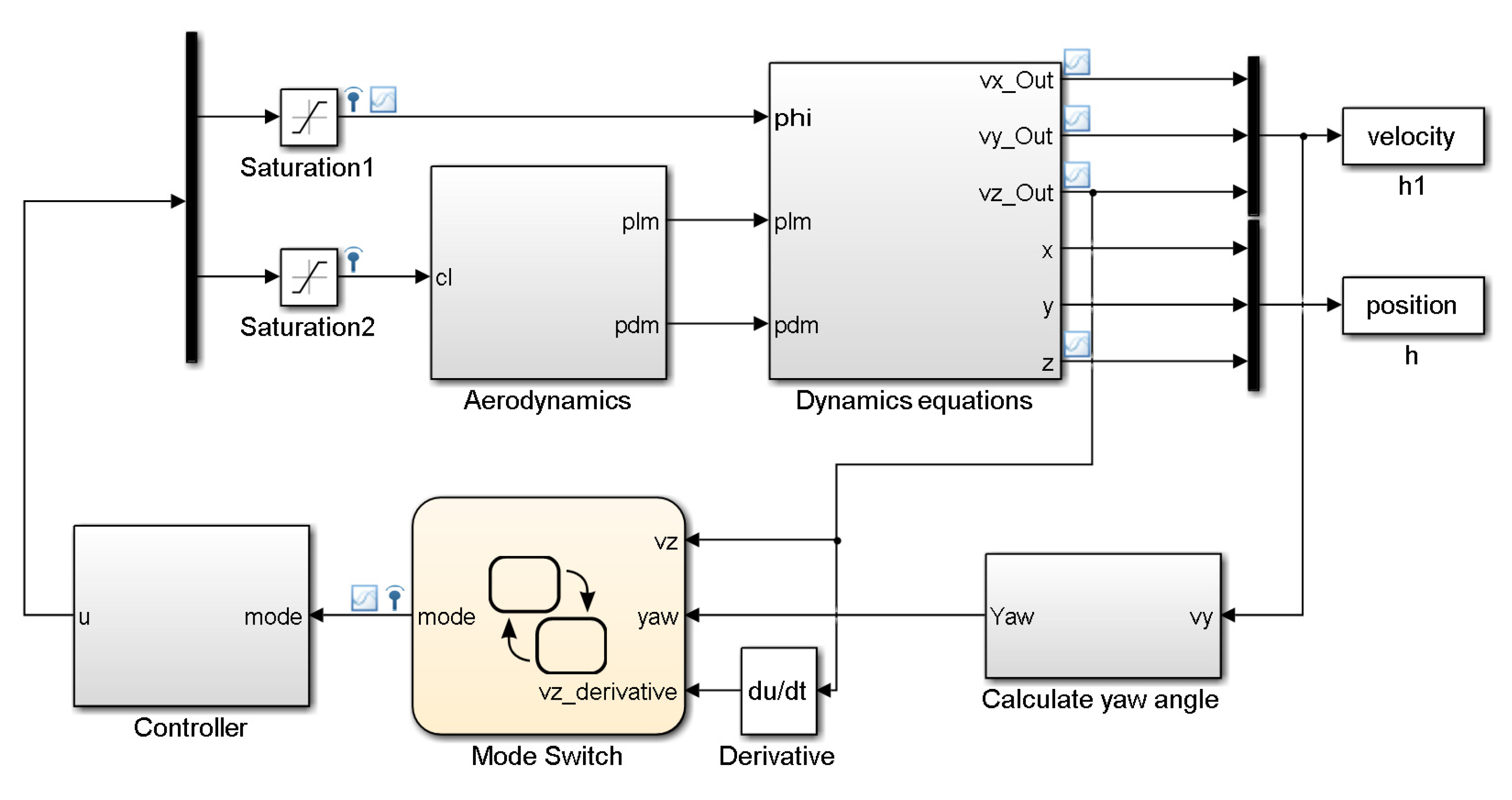
2. Dynamic Model
3. Method for Sustainable Climbing
3.1. Equilibrium Points and Sustainable Climbing
3.2. Proposed Criterion for Unpowered Climbing
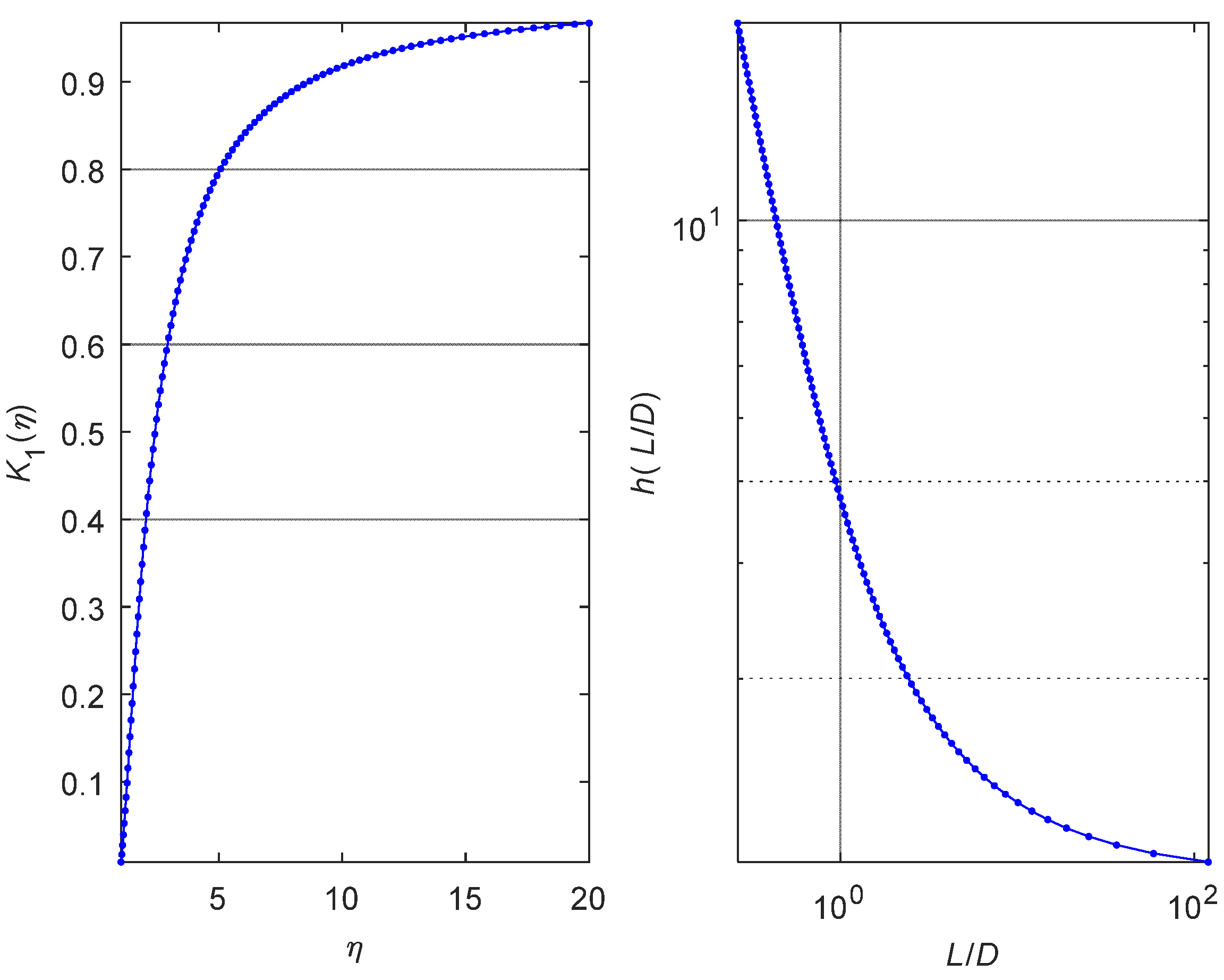
3.3. Derivation of Proposed Criterion
4. Rayleigh Cycle Method
4.1. Energy Perspective
4.2. Optimization Method for Generating Rayleigh Cycle
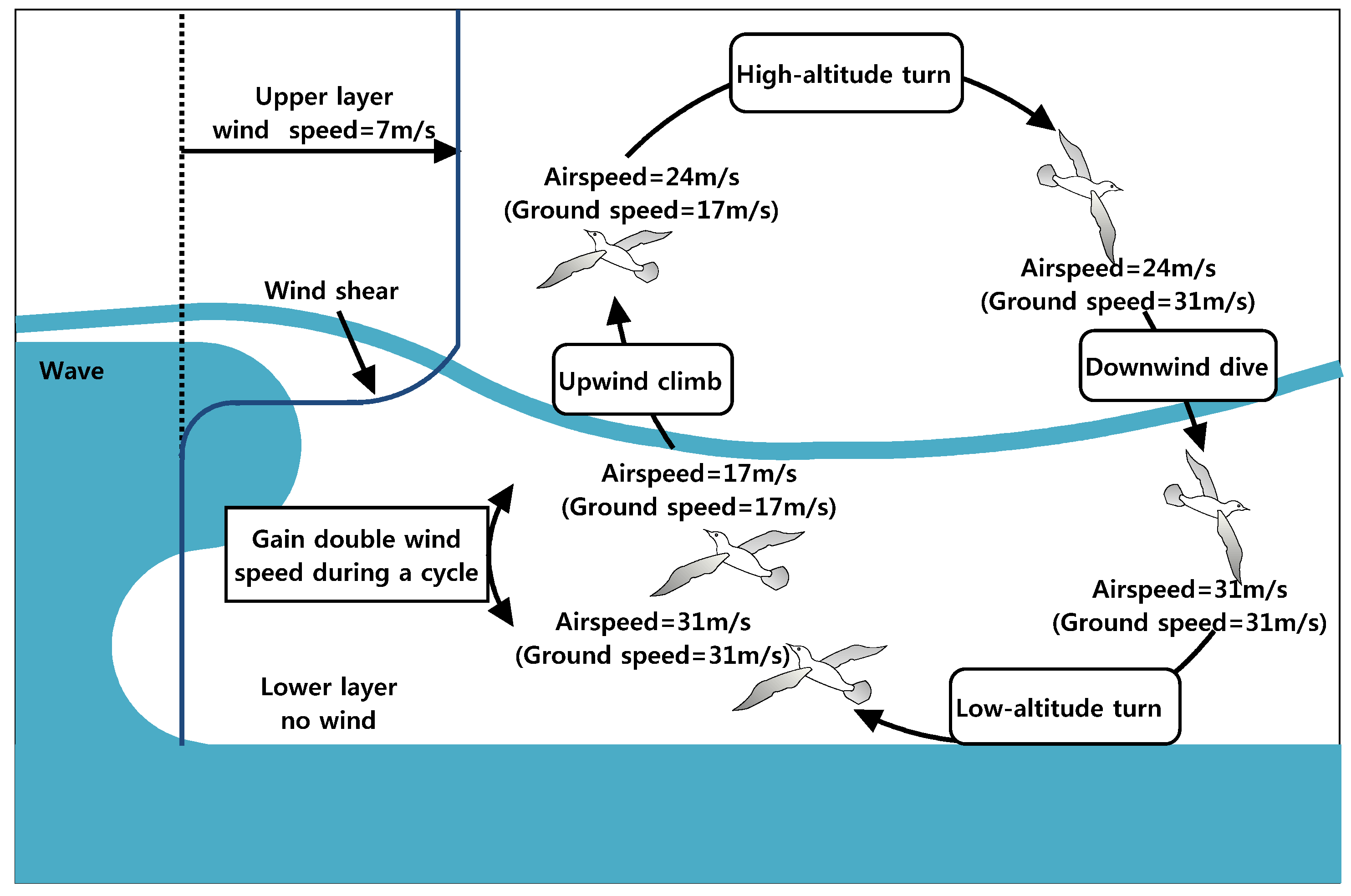
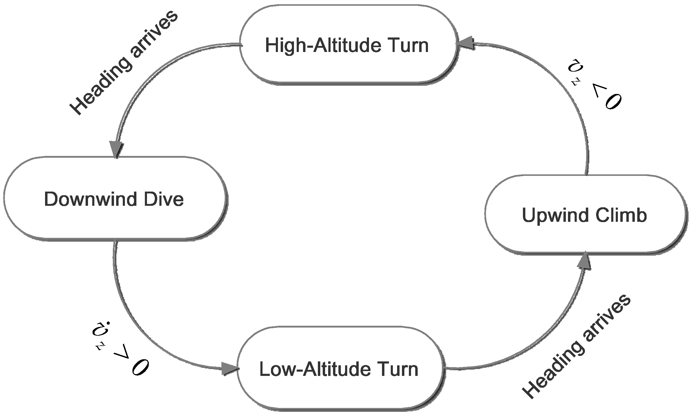
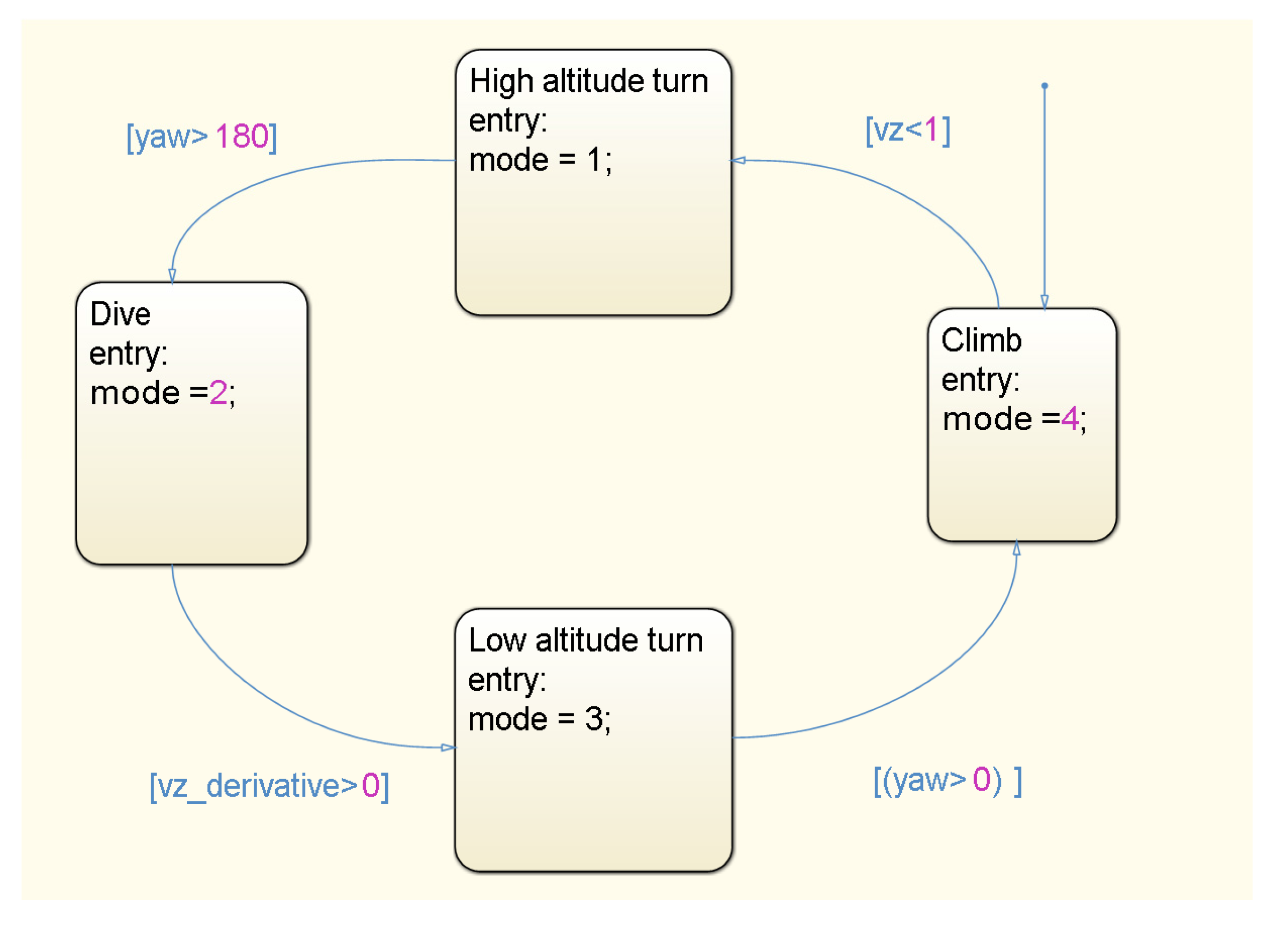
4.3. Bio-Inspired Strategy
4.3.1. Upwind Climb
4.3.2. High-Altitude Turn
4.3.3. Downwind Dive
4.3.4. Low-Altitude Turn
4.3.5. Initial State
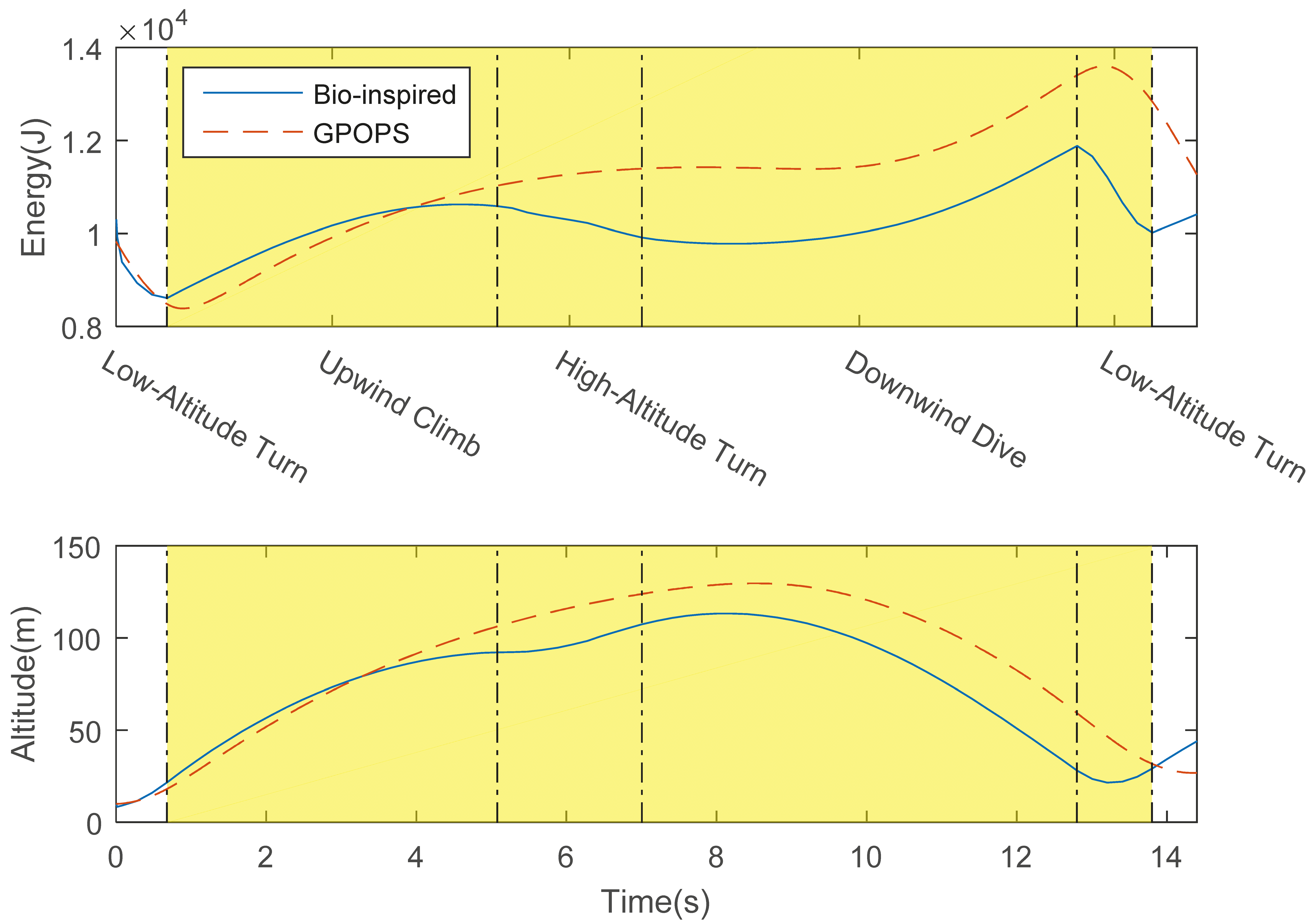
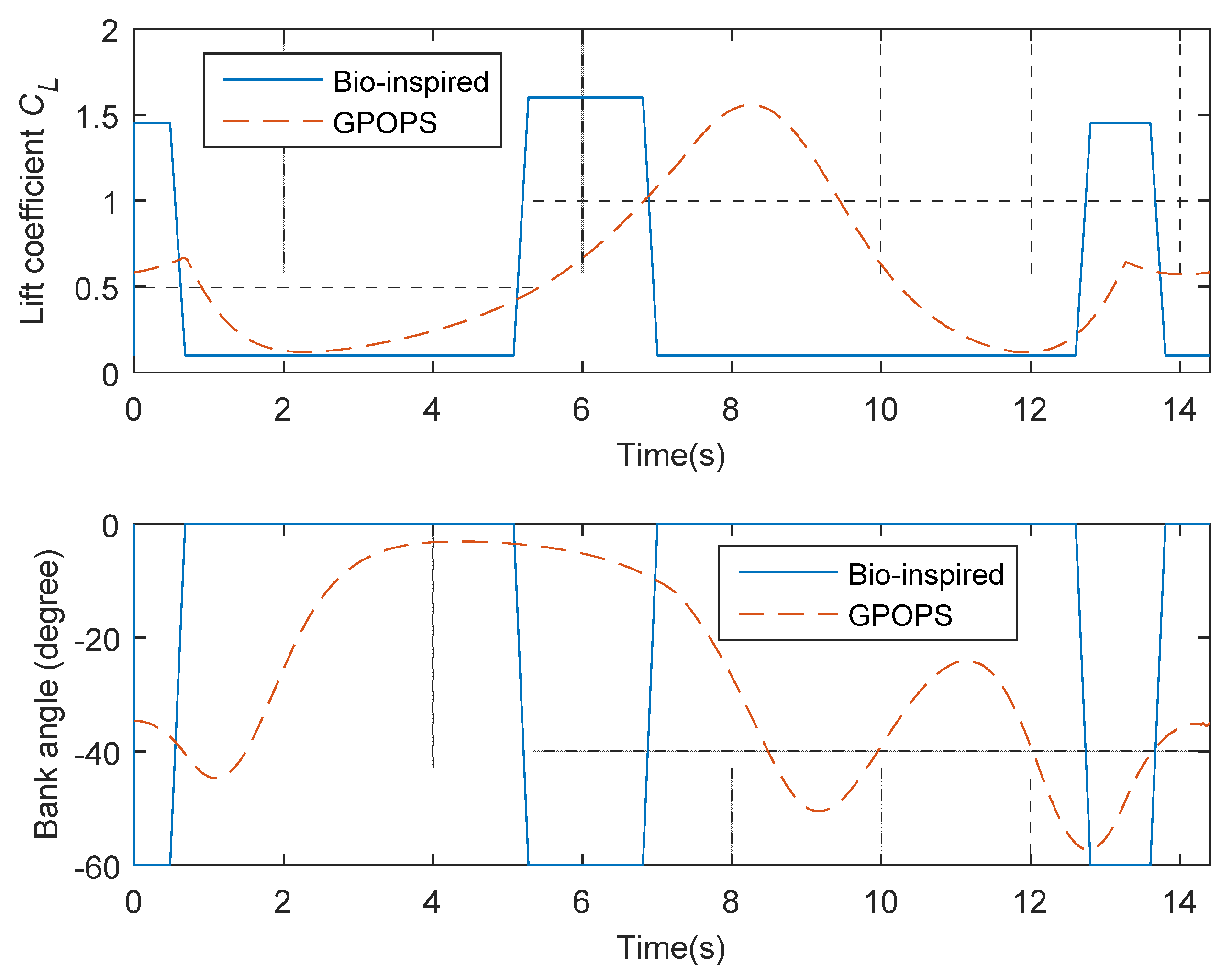
5. Simulation Results and Discussion
5.1. Discussion of Criterion for Unpowered Climbing
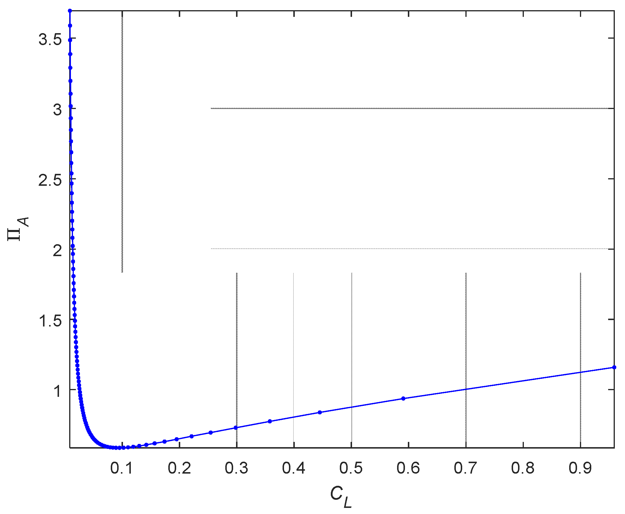
5.1.1. Optimum Lift Coefficient
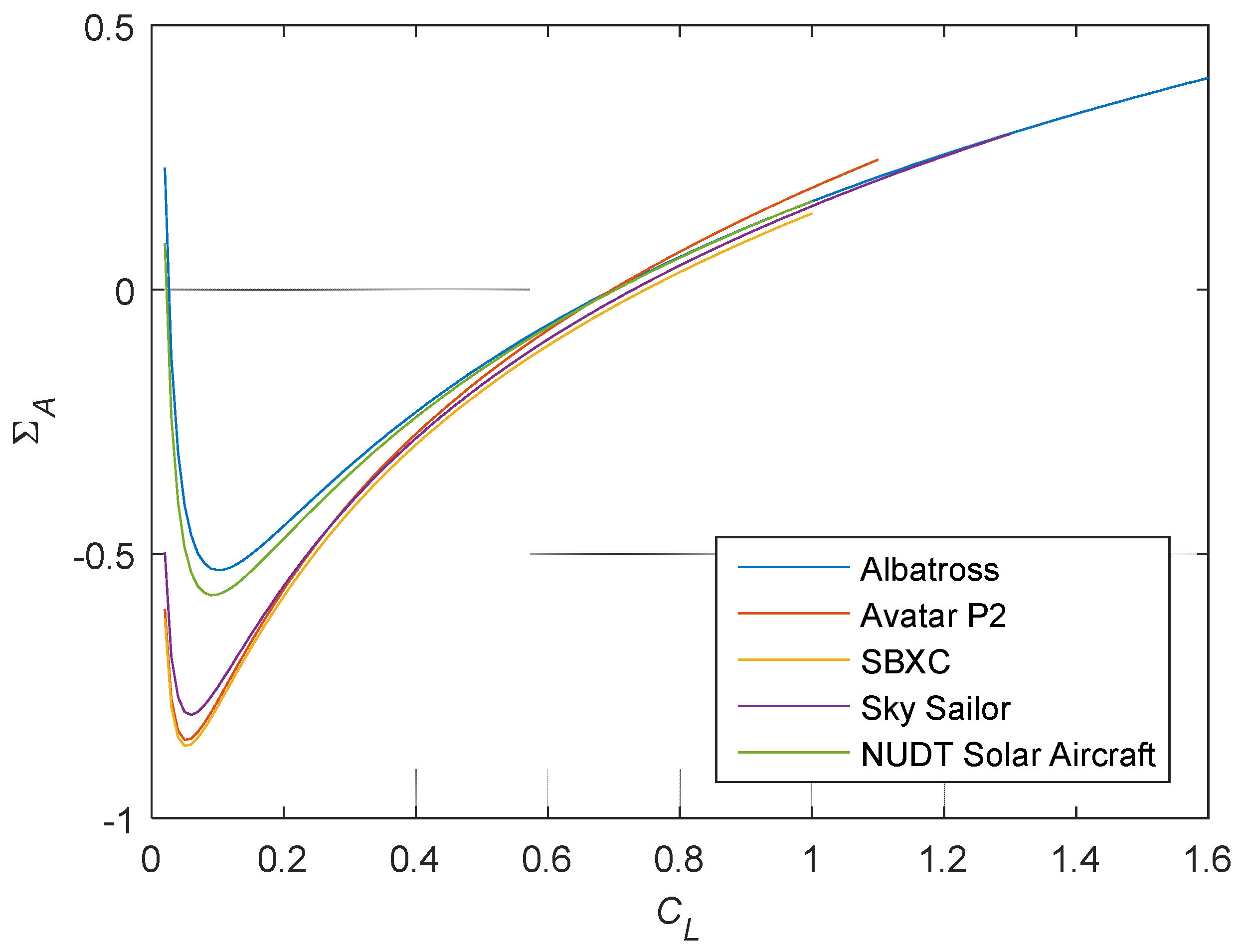
5.1.2. Wing Loading
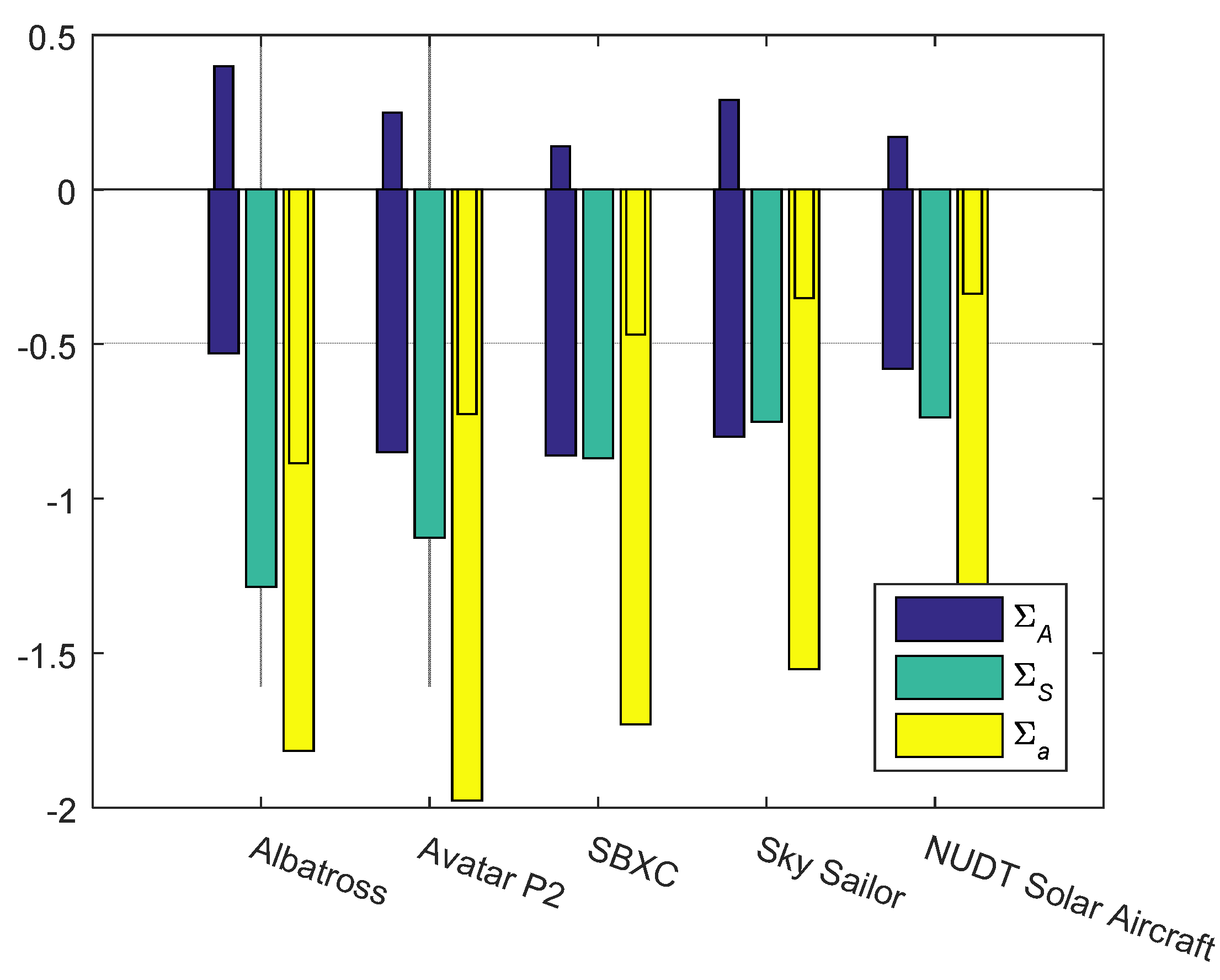
5.1.3. Sensitivity Analysis of Aircraft Fraction
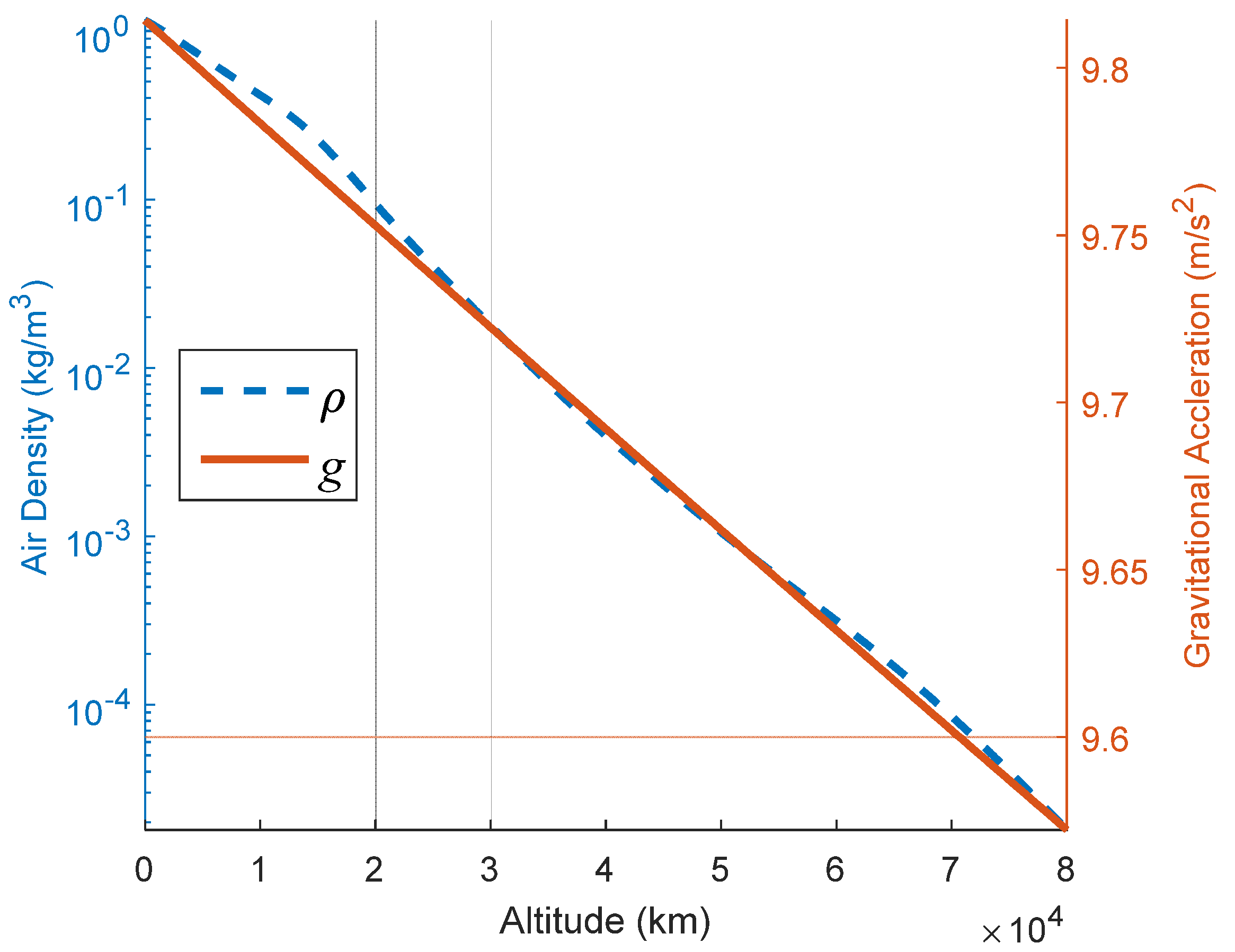
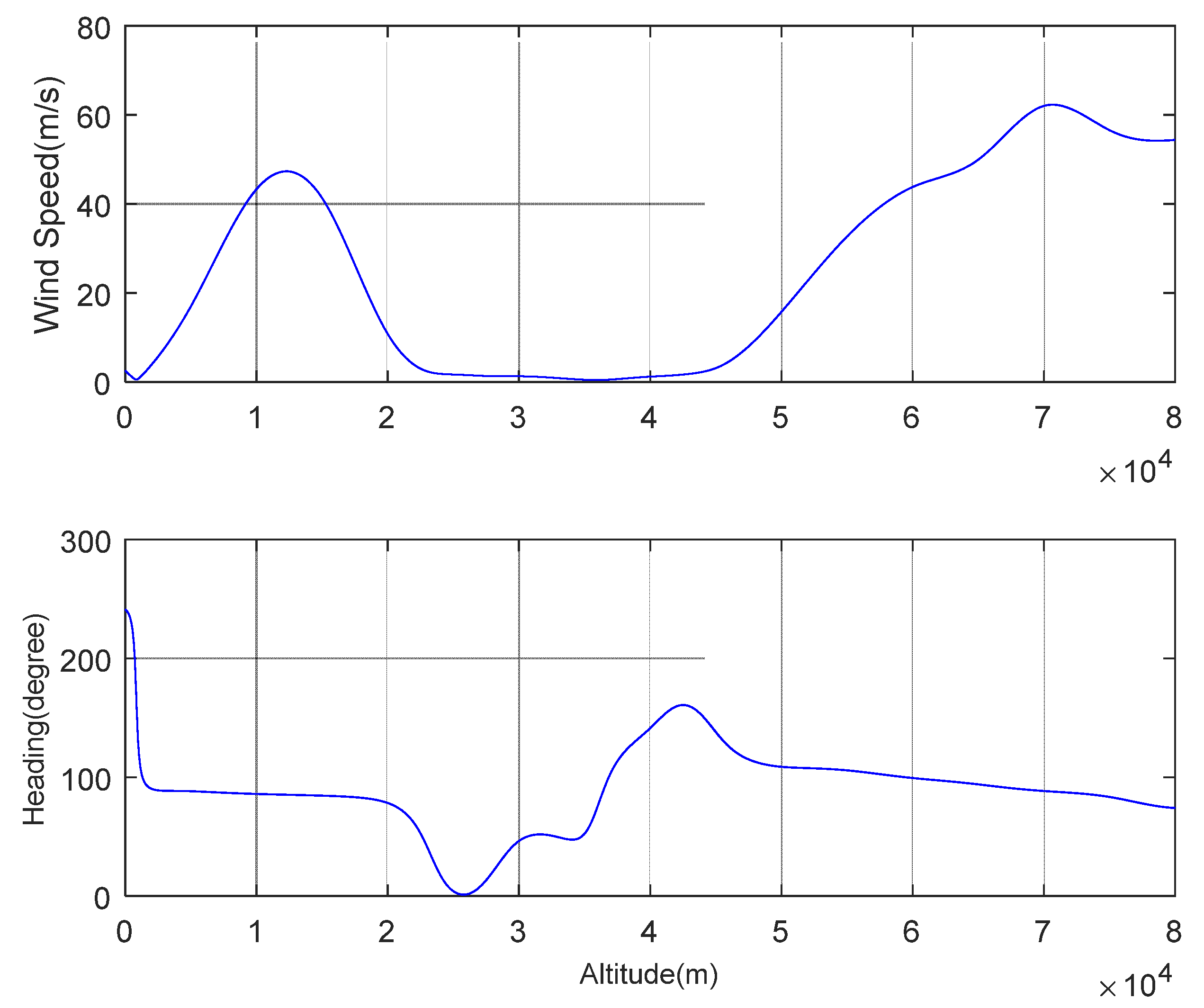
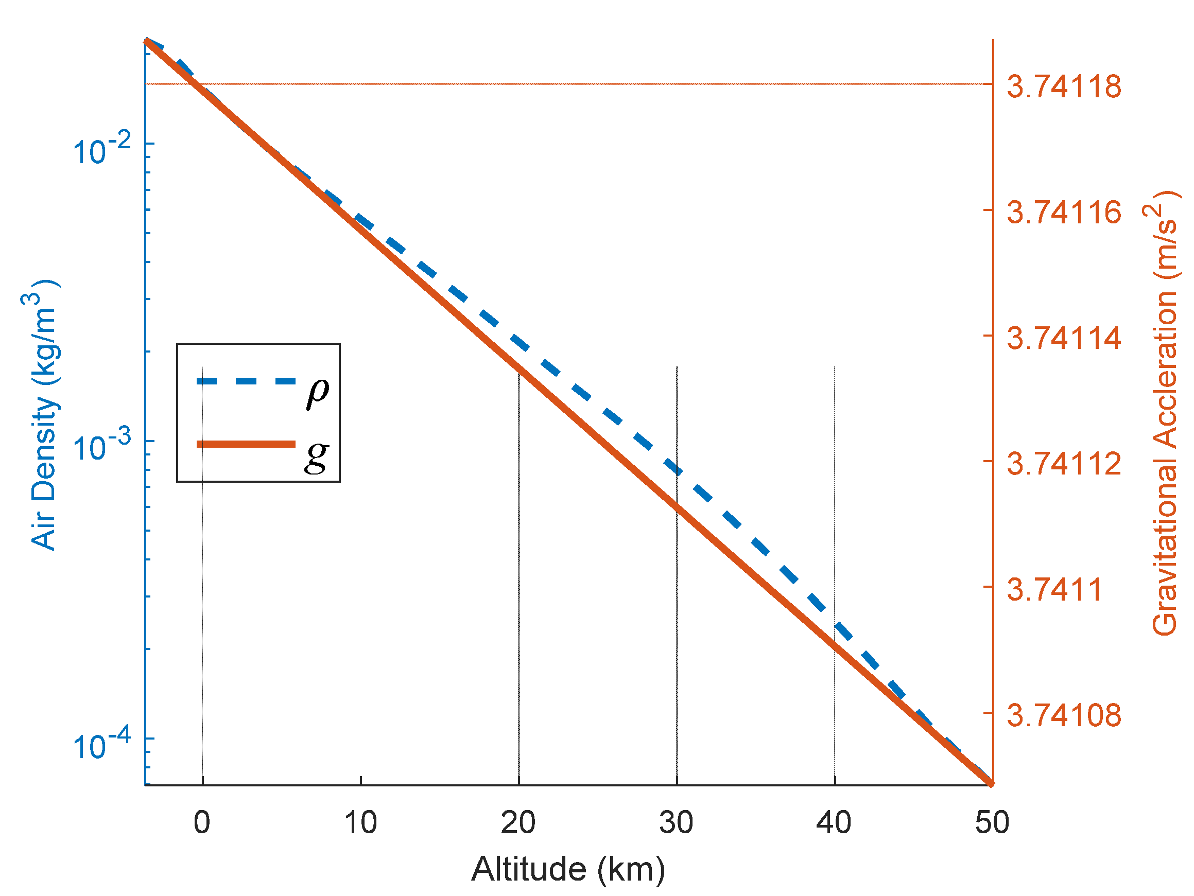
5.1.4. Minimum Gradient and Environmental Effects
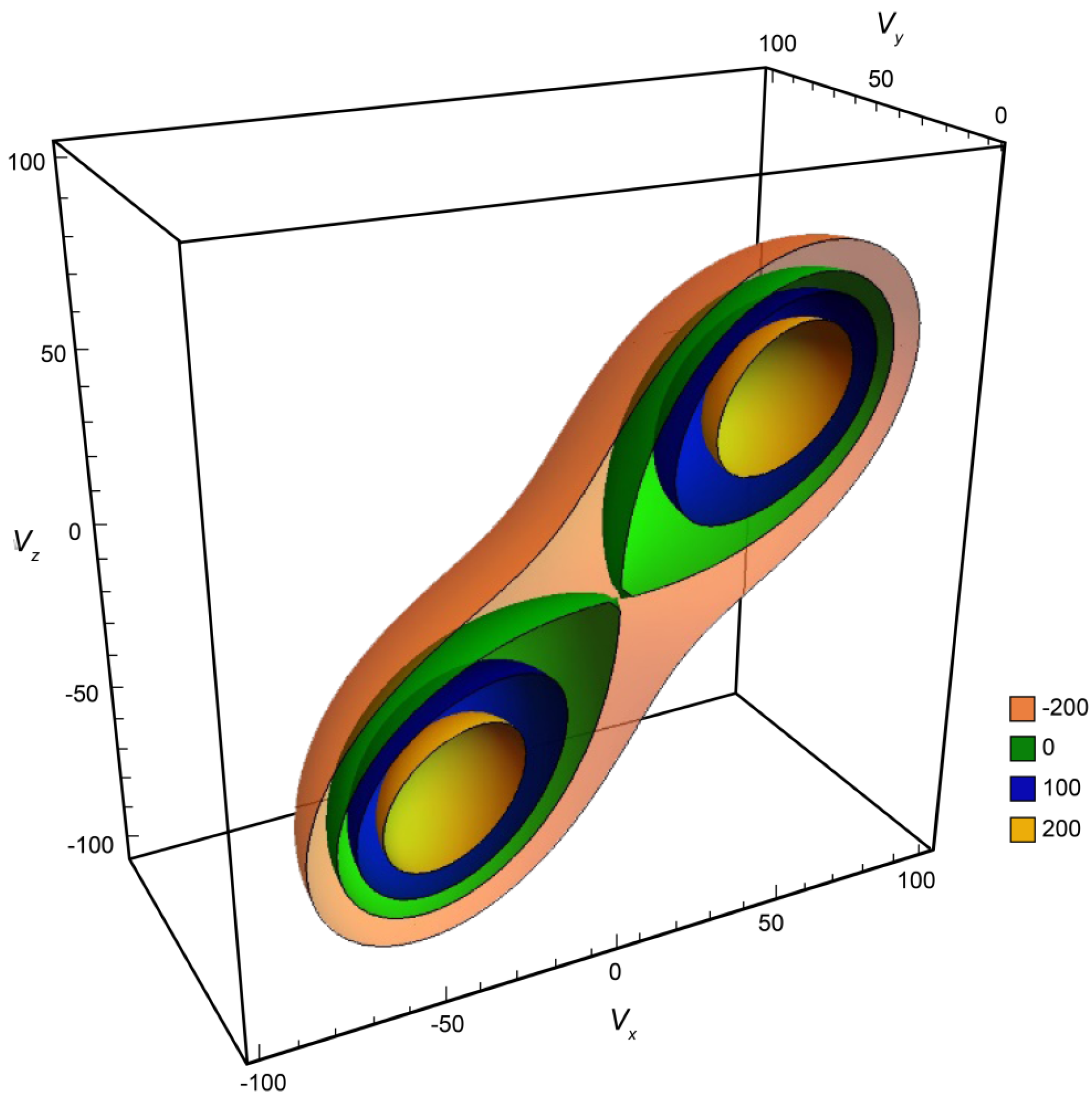
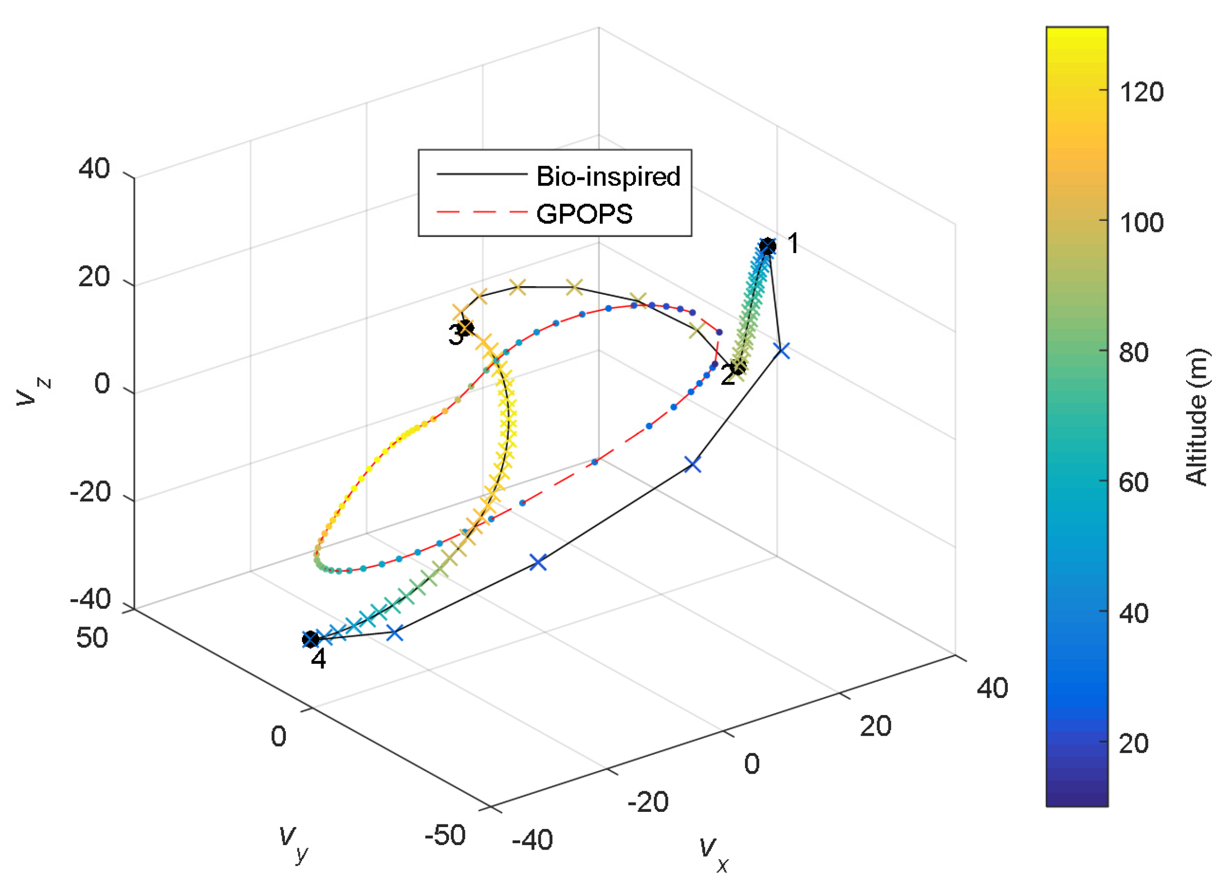
5.2. Rayleigh Cycle Simulation Results
6. Conclusions
Acknowledgments
Author Contributions
Conflicts of Interest
References
- El Alimi, S.; Maatallah, T.; Dahmouni, A.W.; Nasrallah, S.B. Modeling and investigation of the wind resource in the Gulf of Tunis, Tunisia. Renew. Sustain. Energy Rev. 2012, 16, 5466–5478. [Google Scholar] [CrossRef]
- Bonnin, V.; Benard, E.; Moschetta, J.M.; Benard, E. Energy-harvesting mechanisms for UAV flight by dynamic soaring. In Proceedings of the AIAA Atmospheric Flight Mechanics (AFM) Conference, Boston, MA, USA, 19–22 August 2013. [Google Scholar]
- Warrick, D.R.; Hedrick, T.L.; Biewener, A.A.; Crandell, K.E.; Tobalske, B.W. Foraging at the edge of the world: Low-altitude, high-speed manoeuvering in barn swallows. Phil. Trans. R. Soc. B 2016, 371, 20150391. [Google Scholar] [CrossRef] [PubMed]
- Richardson, P.L. How do albatrosses fly around the world without flapping their wings? Prog. Oceanogr. 2011, 88, 46–58. [Google Scholar] [CrossRef]
- Yonehara, Y.; Goto, Y.; Yoda, K.; Watanuki, Y.; Young, L.C.; Weimerskirch, H.; Bost, C.-A.; Sato, K. Flight paths of seabirds soaring over the ocean surface enable measurement of fine-scale wind speed and direction. Proc. Natl. Acad. Sci. USA 2016, 113, 9039–9044. [Google Scholar] [CrossRef] [PubMed]
- Miller, T.A.; Brooks, R.P.; Lanzone, M.J.; Brandes, D.; Cooper, J.; Tremblay, J.A.; Wilhelm, J.; Duerr, A.; Katzner, T.E. Limitations and mechanisms influencing the migratory performance of soaring birds. IBIS 2016, 158, 116–134. [Google Scholar] [CrossRef]
- Sachs, G.; Traugott, J.; Holzapfel, F. In-flight measurement of dynamic soaring in albatrosses. In Proceedings of the AIAA Guidance, Navigation, and Control Conference, Toronto, ON, Canada, 2–5 August 2010. [Google Scholar]
- Airy, H. The soaring of birds. Nature 1883, 28, 103. [Google Scholar] [CrossRef]
- Boslough, M.B. Autonomous Dynamic Soaring Platform for Distributed Mobile Sensor Arrays; Technical Report SAND2002-1896; Sandia National Laboratories: Albuquerque, NM, USA, 2002.
- Idrac, P. Experimental study of the “soaring” of albatrosses. Nature 1925, 115, 532. [Google Scholar] [CrossRef]
- Tucker, V.A.; Parrott, G.C. Aerodynamics of gliding flight in a falcon and other birds. J. Exp. Biol. 1970, 52, 345–367. [Google Scholar]
- Weimerskirch, H.; Guionnet, T.; Martin, J.; Shaffer, S.A.; Costa, D. Fast and fuel efficient? Optimal use of wind by flying albatrosses. Proc. R. Soc. Lond. B Biol. Sci. 2000, 267, 1869–1874. [Google Scholar] [CrossRef] [PubMed]
- Rosen, M.; Hedenstrom, A. Gliding flight in a jackdaw: A wind tunnel study. J. Exp. Biol. 2001, 204, 1153–1166. [Google Scholar] [PubMed]
- Wood, C. The flight of albatrosses (a computer simulation). IBIS 1973, 115, 244–256. [Google Scholar] [CrossRef]
- Hendriks, F. Dynamic soaring in shear flow (of gliders). In Proceedings of the 2nd International Symposium on the Technology and Science of Low Speed and Motorless Flight, Cambridge, MA, USA, 11–13 September 1974. [Google Scholar]
- Denny, M. Dynamic soaring: Aerodynamics for albatrosses. Eur. J. Phys. 2008, 30, 75. [Google Scholar] [CrossRef]
- Taylor, G.K.; Reynolds, K.V.; Thomas, A.L.R. Soaring energetics and glide performance in a moving atmosphere. Phil. Trans. R. Soc. B 2016, 371, 20150398. [Google Scholar] [CrossRef] [PubMed]
- Liu, D.-N.; Hou, Z.-X.; Guo, Z.; Yang, X.-X.; Gao, X.-Z. Bio-inspired energy-harvesting mechanisms and patterns of dynamic soaring. Bioinspir. Biomim. 2016, 12, 016014. [Google Scholar] [CrossRef] [PubMed]
- Zhao, Y.J. Optimal patterns of glider dynamic soaring. Optim. Control Appl. Methods 2004, 25, 67–89. [Google Scholar] [CrossRef]
- Zhao, Y.J.; Qi, Y.C. Minimum fuel powered dynamic soaring of unmanned aerial vehicles utilizing wind gradients. Optim. Control Appl. Methods 2004, 25, 211–233. [Google Scholar] [CrossRef]
- Sachs, G.; Bussotti, P. Application of optimal control theory to dynamic soaring of seabirds. In Variational Analysis and Applications; Springer: Berlin, Germany, 2005; pp. 975–994. [Google Scholar]
- Sachs, G. Minimum shear wind strength required for dynamic soaring of albatrosses. IBIS 2005, 147, 1–10. [Google Scholar] [CrossRef]
- Deittert, M.; Richards, A.; Toomer, C.; Pipe, A. Dynamic soaring flight in turbulence. In Proceedings of the AIAA Guidance, Navigation and Control Conference, Chicago, IL, USA, 10–13 August 2005; pp. 2–5. [Google Scholar]
- Kaushik, H.; Mohan, R.; Prakash, K.A. Utilization of wind shear for powering unmanned aerial vehicles in surveillance application: A numerical optimization study. Energy Procedia 2016, 90, 349–359. [Google Scholar] [CrossRef]
- Yang, H.; Zhao, Y.J. A practical strategy of autonomous dynamic soaring for unmanned aerial vehicles in loiter missions. In Proceedings of the AIAA Infotech@Aerospace, Arlington, VA, USA, 26–29 September 2005; pp. 1–12. [Google Scholar]
- Gordon, R.J. Optimal Dynamic Soaring for Full Size Sailplanes. Master’s Thesis, Defense Technical Information Center, Fort Belvoir, VA, USA, 2006. [Google Scholar]
- Deittert, M.; Richards, A.; Toomer, C.A.; Pipe, A. Engineless unmanned aerial vehicle propulsion by dynamic soaring. J. Guid. Control Dyn. 2009, 32, 1446–1457. [Google Scholar] [CrossRef]
- Akhtar, N.; Whidborne, J.F.; Cooke, A.K. Wind shear energy extraction using dynamic soaring techniques. In Proceedings of the 47th AIAA Aerospace Sciences Meeting Including the New Horizons Forum and Aerospace Exposition, Orlando, FL, USA, 5–8 January 2009. [Google Scholar]
- Du, S.; Gao, Y. Inertial aided cycle slip detection and identification for integrated PPP GPS and INS. Sensors 2012, 12, 14344–14362. [Google Scholar] [CrossRef] [PubMed]
- Lawrance, N.R.; Sukkarieh, S. Autonomous exploration of a wind field with a gliding aircraft. J. Guid. Control Dyn. 2011, 34, 719–733. [Google Scholar] [CrossRef]
- Nguyen, J.L.; Lawrance, N.R.J.; Fitch, R.; Sukkarieh, S. Real-time path planning for long-term information gathering with an aerial glider. Auton. Robots 2016, 40, 1017–1039. [Google Scholar] [CrossRef]
- Langelaan, J.W.; Spletzer, J.; Montella, C.; Grenestedt, J. Wind field estimation for autonomous dynamic soaring. In Proceedings of the IEEE International Conference on Robotics and Automation (ICRA), St. Paul, MN, USA, 14–18 May 2012; pp. 16–22. [Google Scholar]
- Rodriguez, L.; Cobano, J.A.; Ollero, A. Wind field estimation and identification having shear wind and discrete gusts features with a small UAS. In Proceedings of the IEEE/RSJ International Conference on Intelligent Robots and Systems (IROS), Daejeon, Korea, 9–14 October 2016; pp. 5638–5644. [Google Scholar]
- Liu, Y.; Van Schijndel, J.; Longo, S.; Kerrigan, E.C. UAV energy extraction with incomplete atmospheric data using MPC. IEEE Trans. Aerosp. Electron. Syst. 2015, 51, 1203–1215. [Google Scholar] [CrossRef]
- Barate, R.; Doncieux, S.; Meyer, J.A. Design of a bio-inspired controller for dynamic soaring in a simulated unmanned aerial vehicle. Bioinspir. Biomim. 2006, 1, 76. [Google Scholar] [CrossRef] [PubMed]
- Gao, X.Z.; Hou, Z.X.; Guo, Z.; Fan, R.F.; Chen, X.Q. Analysis and design of guidance-strategy for dynamic soaring with UAVs. Control Eng. Pract. 2014, 32, 218–226. [Google Scholar] [CrossRef]
- Yang, Y. Controllability of spacecraft using only magnetic torques. IEEE Trans. Aerosp. Electron. Syst. 2016, 52, 954–961. [Google Scholar] [CrossRef]
- Gao, C.; Liu, H.H.T. Dubins path-based dynamic soaring trajectory planning and tracking control in a gradient wind field. Optim. Control Appl. Methods 2016, 38, 147–166. [Google Scholar] [CrossRef]
- Zhu, B.; Hou, Z.; Shan, S.; Wang, X. Equilibrium positions for UAV flight by dynamic soaring. Int. J. Aerosp. Eng. 2015, 2015, 141906. [Google Scholar] [CrossRef]
- Moorhouse, D.; Woodcock, R. US Military Specification MIL-F-8785C; US Department of Defense: Washington DC, USA, 1980.
- Lift-to-Drag Ratio. Available online: https://en.wikipedia.org/wiki/Lift-to-drag_ratio (accessed on 11 July 2017).
- Rao, A.V.; Benson, D.A.; Darby, C. Algorithm 902: GPOPS, A MATLAB software for solving multiple-phase optimal control problems using the Gauss pseudo spectral method. ACM Trans. Math. Softw. 2010, 1, 2237. [Google Scholar] [CrossRef]
- Anderson, J.D. Fundamentals of Aerodynamics; Tata McGraw-Hill Education: New York, NY, USA, 2010. [Google Scholar]
- McCormick, B.W. Aerodynamics, Aeronautics, and Flight Mechanics; Wiley: New York, NY, USA, 1995; Volume 2. [Google Scholar]
- Noth, A. Design of Solar Powered Airplanes for Continuous Flight. Ph.D. Thesis, ETH Zurich, Zurich, Switzerland, 2008. [Google Scholar]
- Tennekes, H. The Simple Science of Flight: From Insects to Jumbo Jets; MIT Press: Cambridge, MA, USA, 2009. [Google Scholar]
- US Standard Atmosphere; National Oceanic and Atmospheric Administration: Silver Spring, MD, USA, 1976.
- Drob, D.P.; Emmert, J.T.; Meriwether, J.W.; Makela, J.J.; Doornbos, E.; Conde, M.; Hernandez, G.; Noto, J.; Zawdie, K.A.; McDonald, S.E.; et al. An update to the Horizontal Wind Model (HWM): The quiet time thermosphere. Earth Space Sci. 2015, 2, 301–319. [Google Scholar] [CrossRef]
- Gao, X.; Hou, Z.; Guo, Z.; Liu, J.; Chen, X. The influence of wind shear to the performance of high-altitude solar-powered aircraft. Proc. IMechE Part G J. Aerosp. Eng. 2014, 228, 1562–1573. [Google Scholar]
- Braun, R.D.; Wright, H.S.; Croom, M.A.; Levine, J.S.; Spencer, D.A. Design of the Ares Mars airplane and mission architecture. J. Spacecr. Rocket. 2006, 43, 1026–1034. [Google Scholar] [CrossRef]
- Guynn, M.; Croom, M.; Smith, S.; Parks, R.; Gelhausen, P. Evolution of a Mars airplane concept for the Ares Mars scout mission. In Proceedings of the 2nd AIAA Unmanned Unlimited Systems, Technologies, and Operations Conference, San Diego, CA, USA, 15–18 September 2003. [Google Scholar]
- Noth, A.; Bouabdallah, S.; Michaud, S.; Siegwart, R.; Engel, W. Sky-Sailor design of an autonomous solar powered Martian airplane. In Proceedings of the 8th ESA Workshop on Advanced Space Technologies for Robotics, Noordwick, The Netherlands, 2–4 November 2004. [Google Scholar]
- Anyoji, M.; Nagai, H.; Asai, K. Development of low density wind tunnel to simulate atmospheric flight on Mars. In Proceedings of the 47th AIAA Aerospace Sciences Meeting Including the New Horizons Forum and Aerospace Exposition, Orlando, FL, USA, 5–8 January 2009. [Google Scholar]
- Murray, J.E.; Tartabini, P.V. Development of a Mars Airplane Entry, Descent, and Flight Trajectory; NASA/TM-2001-209035; NASA Dryden Flight Research Center: Edwards, CA, USA, 2001.
- Justus, C.G.; Duvall, A. Mars aerocapture and validation of Mars-GRAM with TES data. In Proceedings of the 53rd JANNAF Propulsion Meeting, Monterey, CA, USA, 5–8 December 2005. [Google Scholar]


| State | νx | ||
|---|---|---|---|
| >0 | <0 | ||
| νz | >0 | Upwind Climb | Low Altitude Turn |
| <0 | High Altitude Turn | Downwind Dive | |
| Aircraft | Albatross [22] | Avatar P2 [23] | SBXC [30] | Sky Sailor [45] | NUDT Solar Aircraft |
|---|---|---|---|---|---|
| S (m2) | 0.65 | 0.473 | 0.957 | 0.78 | 1.56 |
| m (kg) | 8.5 | 4.5 | 5.443 | 2.5 | 6.8 |
| CD0 | 0.033 | 0.0173 | 0.017 | 0.0191 | 0.03 |
| N | 0.019 | 0.0517 | 0.0192 | 0.0268 | 0.0223 |
| (CL)max | 1.6 | 1.1 | 1.0 | 1.3 | 1.0 |
| m/S (kg/m2) | 13.08 | 9.51 | 5.69 | 4.49 | 4.36 |
| Method | GPOPS | Bio-Inspired Strategy |
|---|---|---|
| Computation time | 15 s | 2 ms |
© 2017 by the authors. Licensee MDPI, Basel, Switzerland. This article is an open access article distributed under the terms and conditions of the Creative Commons Attribution (CC BY) license (http://creativecommons.org/licenses/by/4.0/).
Share and Cite
Shan, S.; Hou, Z.; Zhu, B. Albatross-Like Utilization of Wind Gradient for Unpowered Flight of Fixed-Wing Aircraft. Appl. Sci. 2017, 7, 1061. https://doi.org/10.3390/app7101061
Shan S, Hou Z, Zhu B. Albatross-Like Utilization of Wind Gradient for Unpowered Flight of Fixed-Wing Aircraft. Applied Sciences. 2017; 7(10):1061. https://doi.org/10.3390/app7101061
Chicago/Turabian StyleShan, Shangqiu, Zhongxi Hou, and Bingjie Zhu. 2017. "Albatross-Like Utilization of Wind Gradient for Unpowered Flight of Fixed-Wing Aircraft" Applied Sciences 7, no. 10: 1061. https://doi.org/10.3390/app7101061
APA StyleShan, S., Hou, Z., & Zhu, B. (2017). Albatross-Like Utilization of Wind Gradient for Unpowered Flight of Fixed-Wing Aircraft. Applied Sciences, 7(10), 1061. https://doi.org/10.3390/app7101061