Abstract
As a key concern in a power system, a deteriorated insulation is likely to bring about a partial discharge phenomenon and hence degrades the power supply quality. Thus, a partial discharge test has been turned into an approach of significance to protect a power system from an unexpected malfunction. An improved Hilbert–Huang Transformation (HHT) is proposed in this work as an effective way to address the issues of an optimal shifting number and illusive components, both suffered in a conventional HHT approach, and is then applied to a defect mode recognition for a partial discharge signal analysis in the case of a cross-linked polyethylene insulated power cable. As the first step, the partial discharge signal detected is converted through the proposed improved HHT to a time-frequency-energy 3D spectrum. Then as the second step, the fractal features contained therein are extracted by way of a fractal theory, and in the end the defect modes are recognized as intended by use of an extension method.
1. Introduction
As technology development progresses and improved living standards are promoted, there is a corresponding and growing demand for power quality in human society. As an essential facility in all sections of industries, a power system influences economic growth or human’s daily life, from something as little as a power outage, to something far more serious, such as severe damage to power generation and transmission equipment, or even an entire power network shut down, which would be a tremendous thread to the power system [1,2]. For the sake of maintaining a quality power system, the performance as well as the reliabilities of a power transmission line and high low voltage equipments is a critical issue. A power system is mainly made up of conductors, ferrite materials and insulators, namely the key component for a well maintained power system, simply for the reason that a deteriorated insulator is commonly seen in an overloaded or aged facility. In addition, human errors or construction not following a standard operating procedure are also found as further cause for a damage to an insulator. Statistics show that a large number of accidents in the course of power system operation are attributed to aged or malfunctioned insulators [3,4].
According to the literature [5,6], the different types of partial discharge (PD) sources can generate different discharge patterns. The discharge pattern is represented by a set of characteristic features, which can be extracted from a PD signal. In the early days, a partial discharge signal was recognized by seasoned specialists according to the features revealed on an elliptical trajectory. However, as a consequence of a long term technology progress made over years, commercial instruments have been made to accurately sense partial discharge signals [7,8,9] emanating from an insulation facility, analyze the dielectric punch through process, provide a maintenance message and prevent catastrophe. Yet, such commercial instruments, valued as high as a million dollars, preprocess field detected signals in their front end circuits, and as a results, part of the intrinsic physical meaning contained is lost. For this reason, a detected signal is transformed into a time–frequency–energy 3D spectrum through the improved Hilbert–Huang Transformation (HHT), combined with a fractal theory to extract fractal features embedded. Finally, an extension method is adopted so as to identify defect modes out of a partial discharge signal.
Subject to the defect types of an insulator, a partial discharge process is a highly complicated phenomenon, that is, distinct defect models bring about distinct discharge spectrums as expected. In a bid to accurately recognize insulation conditions of a power cable, a data base is built for diagnosis purposes by successively measuring partial discharge signals from a sequence of defect models. This work aims to analyze a detected discharge signal through the Hilbert–Huang transform, an approach with a high resolution to a nonlinear as well as non-stationary signal. Yet, there exist two inherent problems, degrading the accuracy in signal analysis and hence a barrier to an automatic defect mode identification. The first problem is lacking a decision criterion to precisely specify the optimal shifting number. In the case of an excessive shifting number, the intrinsic physical meaning carried in extracted intrinsic mode function (IMFs) will be unintentionally removed, that is, any instant frequency cannot be viewed out of all the IMFs accordingly. The second is that illusive components may be seen in the course of empirical mode decomposition (EMD) process as a result of the use of the extrema interpolation, i.e., a cause for a mode confusion problem.
For this sake, combined with a K-S test and an energy ratio sorting, an improved HHT, abbreviated as IHHT hereafter, is proposed as an effective approach to specify the optimal shifting number and as a decision criterion in the identification of illusive components. With the optimal shifting number, each IMF is purified, then illusive components are filtered out according to the decision criterion, and in the end, the accuracy of the Hilbert spectrum is thus improved. For the reason that feature extraction cannot be performed with little effort out of a Hilbert spectrum, the automatic identification of partial discharge defect modes is performed on a time–frequency–energy 3D spectrum, a spectrum converted from the Hilbert spectrum. Consequently, four features, namely fractal dimension, mean energy and mean discharged energy, are extracted as a prerequisite of the identification task. As put forward in a prior work of ours [10,11], various defect modes make various contribution to the discharge duration, the discharge frequency and the discharged energy. Even though types of malfunctions can be identified in an effective manner by making good use of the features, i.e., fractal dimension, and mean energy, there is still room left for further improvement. Defined exclusively in IHHT as the average of the total energy distributed over the entire Hilbert spectrum, the average energy is adopted as a way to elevate the identification ratio, due to the fact that distinct defect mode demonstrates distinct amount of energy on the Hilbert spectrum.
2. Hilbert–Huang Transform
2.1. Empirical Mode Decomposition
EMD is an approach in which a complicated signal can be expressed as the sum of n number of intrinsic mode functions (IMF). Identifying the features contained in respective IMFs in an effective manner, EMD demonstrates a high adaptivity in the aspect of nonlinear as well as non-stationary signal analyses [12].
It is postulated in an EMD analysis that an arbitrary signal x(t) can be written as the sum of a number of IMFs, each reflecting the physical meaning over respective spectral band. A typical IMF must satisfy two of the underlying conditions. The first condition is that there exist the same number of extremums as zero crossing points, or a maximum difference of unity between such two numbers, while the second is that the upper and the lower envelopes, covering all the local maximum and minimum points, respectively, and exhibit a zero mean.
An EMD decomposition is made through the following steps. As the first step, all the local extremum points must be located, then concatenated via cubic splines so as to form the upper and the lower envelopes respectively [13,14]. The mean m10 between such two envelopes is evaluated as
In case h10 does satisfy the IMF definition, h10 is treated as the first IMF. If not, the above step is iterated with h10 as the initial value until the maximum shifting number k is reached or the IMF definition is satisfied.
Empirically, it is very unlikely to make h1k satisfy the IMF definition in the course of decomposition, meaning that it takes the maximum number, k, of iterations to terminate the decomposition process. Consequently, a critical issue of the precise determination of the optimal shifting number in each IMF is detailed as follows.
Subsequently, letting c1=h1k, c1 is extracted out of x(t), and r1, the updated signal, is given as
Performing n times of the above iterations leads to n IMFs, presented as
Such iteration terminates in the event that no more IMF can be found for a monotonic function rn. Derived from (3) and (4), the EMD decomposition is represented as
2.2. Hilbert Spectrum
Based on the local characteristic timescale of the signal, EMD decomposes a signal into n IMFs as intended, such that an instant frequency reflects certain type of physical meaning. Taking the Hilbert transform of (5), ci(t) is transformed into [14]
Construct an analytical signal
And then an amplitude function is given as
An instantaneous phase function is as
The instantaneous frequency is represented as
And the Hilbert spectrum is denoted as
Without taking the residual rn into account, and with RP standing for the real part of a complex operand. A superior adaptivity is seen for a partial discharge analysis made by HHT due to the nature of a nonlinear as well as non-stationary signal. As referred to previously, intrinsic physical meaning is revealed respectively by instant frequencies such that a deteriorated insulation can be detected in early stage.
3. Improved HHT
In an attempt to definitely specify the optimal shifting number and rid illusive components, an improved version of HTT is proposed as follows.
3.1. Kolmogorov-Smirnov Test
A Kolmogorov-Smirnov (K-S) test is conducted as a way to view the difference of probability distributions between two distinct sets of data. Assuming y(n) = {y1, y2, y3, … , yn}, a cumulative distribution function (CDF) is defined as [15,16]
where n(i) denotes the number of samples, less than y(n), permuted into ascending order. Symbolizing the cumulative distribution function (CDFs) of two signals as Fn(x) and F0(x) respectively, the maximum deviation D is given as
Furthermore, the similarity probability P between two tested signals is evaluated as
where
A near zero λ implies a near unity K(λ), while a λ approaching ∞ indicates a K(λ) close to zero. Thus, a similarity probability close to unity represents a high similarity between signals, but a nearly zero similarity probability denotes a considerable distinction between CDFs. The fundamental criterion in a K-S test is improved in such a way that the optimal shifting number can be definitely specified and all the illusive components are removed, as will be portrayed in the following sections.
3.2. Signal–Energy Ratio Method
For the purpose of an accurate decomposition of a practical discharge signal in HTT, there is an optimal shifting number required to preserve the intrinsic physical meaning. Treated as the fundamentals of the decision criterion, the signal power ratio between IMFs is defined as
where n represents the number of IMFs, t the time instant of signal, and x(t) an original signal. The clear advantage gained over a conventional K-S test is that a relatively high precision is seen in respects of frequency, distribution and energy, and a relatively high similarity is demonstrated as a consequence of a short duration of the partial discharge signal. The optimal shifting number is found by means of a K-S test and pn sorting to locate the true components according to the consistency between the sorting between the probability distributions and energy ratios. Thus, the EMD decomposition is indeed an approach not merely able to allocate respective spectral bands to corresponding IMFs, but also, able to well preserve all the intrinsic physical meanings.
3.3. Optimal Shifting Number
As illustrated in Figure 1, the decision criterion of the optimal shifting number is made by a comparison test whether the K-S test result matches the sorting by the signal energy ratio. The filtration of a trend curve, i.e., the removal of non electric noise, is made as an effective prerequisite to promote the accuracy of an HTT analysis.
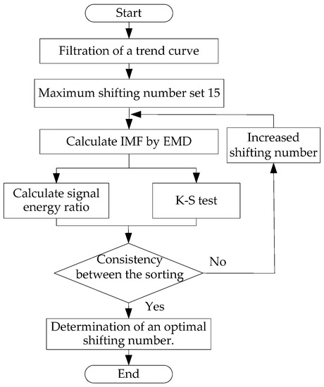
Figure 1.
Flowchart for the determination of an optimal shifting number.
3.4. Judgment of Illusive Component
As a consequence of both the upper and lower envelopes identified by means of extrema interpolation, illusive components are seen in IMFs in the course of an EMD decomposition. It is hence postulated that the HTT accuracy can be upgraded in case all the illusive components can be identified and filtered out in an effective manner. Underlain by a K-S test, an iterative decision criterion is proposed in this work to address the threshold value problem as put forward by the authors of [17]. Subsequent to the EMD decomposition, n number of IMFs are gained and respective similarity probabilities, evaluated by the K-S test, sorted in a descending order, are added up in sequence. In the case of true IMF components, a cumulative similarity probability between the added up and the original signals is seen toward unity. If this is not the case, a decreasing trend of the similarity probability is deemed as the case of illusive components. This decision criterion is made to identify each IMF as either an illusive or a true component, that is, each IMF, not containing the intrinsic physical meaning of a partial discharge signal, is treated as an illusive component, and vice versa. Demonstrated in Figure 2 is a criterion flow chart of the illusive component decision.
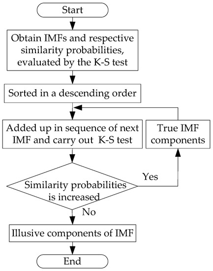
Figure 2.
Judgment criterion of illusive components for a cumulative test.
As illustrated in Figure 3, the trend curve embedded in a partial discharge signal detected on site is requested to be filtered out as the first step of EMD process in an attempt to upgrade the accuracy of HTT analysis. The resultant signal is then treated as an updated signal for the second run of the EMD process in determination of the optimal shifting number. The last step is the removal of illusive components.
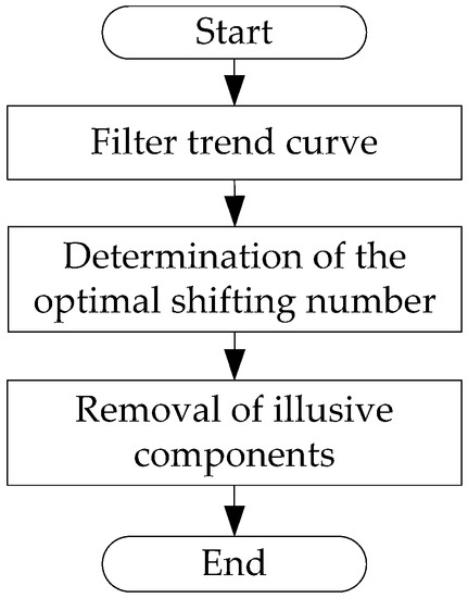
Figure 3.
Analysis flow of improved Hilbert–Huang Transformation (HHT).
4. PD Recognition System
Numerous underground cables exist for the power distribution level in urban areas. Defects in cable may cause PD phenomena and infect power supply reliability. Therefore, this study establishes four defect types of cable joints frequently encountered in the on-site construction phase. The proposed inspection method should be able to determine the insulation quality of a cable joint, and can be used by the construction unit to verify the quality of the cable joint and provide training materials for construction taskforces. Ideally, this approach can help prevent similar construction defects in the future.
4.1. Experiment Model
Statistics in the literature indicate that a high proportion of the cross-linked polyethylene (XLPE) power cable breakdowns occur in cable joints [18,19]. The experimental objects in this study were 25 kV XLPE power cable joints. Figure 4 shows the possible defect models that may be caused by humans during power cable joint construction. This study simulates an insulation defect caused by a knife when the worker peeled the insulation shield. The defect depth is 2 mm and length is 20 mm in insulation, defined as XLPE insulation with a knife defect (Type I). In our experiment, the normal length of the insulation shield to the conductor terminal should be cut to 139 mm, with ±10% being an acceptable range. We simulated that worker cut to 167 mm, which is 20% more than the normal length, and was defined as the insulation shield being too short (Type II). Another simulated insulation shield cut only 111 mm, which is 20% less than the normal length, and was defined as the insulation shield being too long (Type III). A healthy power cable joint (Type IV). Defect in cable terminal connector (Type V). Finally, a healthy terminal connector (Type VI).
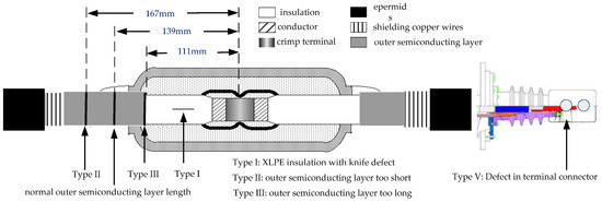
Figure 4.
Experimental defect models in XLPE power cable.
4.2. Measurement Environment
Figure 5 shows a block diagram of the PD experiment in the laboratory. Construction of the PD experiment laboratory included a notebook (NB), high voltage control panel, an isolation transformer, a step-up transformer, test objects (power cable), a data acquisition (DAQ) card and a high-frequency inductive sensor (L sensor) to measure the electrical signal caused by the PD phenomenon in power cable. This experiment used the positive edge trigger function of the DAQ card to acquire the output voltage of the isolation transformer as the trigger signal. The electrical signals recorded by the L sensor were all synchronized in each experimental model.
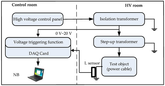
Figure 5.
Block diagram of partial discharge (PD) measurement experiment.
In the voltage step-up procedure of the PD experiment, a 25 kV cable should have 14.4 kV(U0) rated phase to ground voltage. However, according to IEC 60502-2 for a power cable from 6 kV to up to 30 kV, the test after installation voltage should be 1.7 U0 for 5 min [20]. Because the voltage must exceed the partial discharge inception voltage to excite the PD phenomenon, the testing voltage should be 1.7 × 14.4 kV = 24.5 kV. Thus, 25 kV was selected as the test voltage. The high voltage generator generated a rising voltage from 0 V to 25 kV. The inductive (L) sensor then measured the power cable joint and recorded the signals after 1 min. During the experimental process, the sampling rate was set at 20 M/s to acquire one power cycle (60 Hz) acoustic signal. All measured signals determined through the preamplifier and analog data were converted to digital data for storage in a computer. In the general practice of PD tests, a longer period of measurement is advantageous in PD identification. Because the experimental model of this study was established based on the common defect patterns of cable joints and the measurements were conducted in a shielded environment of a laboratory, clear PD signals could be measured for each single cycle. Therefore, only one cycle was taken for signal processing in this study. A longer sampling time should be taken for signal processing in practical PD measurement in the future.
4.3. Feature Extraction
Researchers have successfully used fractal theory to address the problem of modeling and describe complex shapes. This technique has potential for the classification of textures and objects present in images and natural scenes, and for modeling complex physical processes [21]. This study extracts the feature parameters of the fractal features from the 3D Hilbert energy spectrum. Fractal features, fractal dimension, and lacunarity were extracted to highlight the more detailed characteristics of raw 3D patterns.
4.3.1. Fractal Dimension
The definition of fractal dimension by self-similarity is straightforward, where self-similar means they are the same from near as from far, it is often difficult to be either estimated or computed for a given image data. However, a relevant measure of fractal dimension, the box dimension, can be more efficiently computed instead. In this work, suggested by Voss, the method has been followed for the computation of fractal dimension D from the image data. Define p(m,L) as the probability that there are m points within a box of size L, i.e., a cube of side L, centered about a point on the image surface. p(m,L) is normalized for all L, expressed as [21]
where Nb represents the number of possible points within the box. Letting S be the number of image points (i.e., pixels in an image), there are (S/m) p(m,L) number of boxes with m points inside the box in case the image is overlaid with boxes of side L. Therefore, the expected number of boxes in total required to cover the whole image [22] is given as
This value is found to be proportional to L−D, according to which the box dimension can be estimated by calculating p(m,L) and N(L) for various values of L, and subsequently by performing a least square fitting on {log(L),-log(N(L))}. In an attempt to evaluate p(m,L), the cube of size L must be centered around an image point, and the neighboring m points, that fall within the cube, must be counted. The occurrences of each number of neighboring points over the image are accumulated in the determination of the occurrence frequency of m, which is normalized to obtain p(m,L).
4.3.2. Lacunarity
The ideal fractal is likely to confirm to statistical similarity for all scales, that is, fractal dimensions are all independent scales. However, fractal dimension alone is found insufficient for discrimination purposes, since two distinct surfaces could share the same value of D. To circumvent this, the term lacunarity (Λ), introduced by Mandelbrot, is used to quantify the denseness of an image surface. Since then, there have been various definitions for this term proposed to quantify the gaps or lacunae present in a given surface. As suggested by Mandelbrot [23], the term is defined as
where N is the number of points in the data set of size L, the lacunarity can be defined as
Figure 6 shows the procedure for extracting fractal features. The first step of fractal dimension computation is to transfer the 3D Hilbert energy spectrum to a 256 × 1024 scale image matrix. This study chooses sizes L = 2, 3, 4, 5, 6, and 8 because testing revealed them to be suitable for this application. Using different box sizes L enables obtaining different forms of N(L). Finally, fitting the data {log(L),-log(N(L))} yields the fractal dimension. In a lacunarity computation, the first step is to transfer the 3D Hilbert energy spectrum to a 256 × 1024 binary image matrix. The chosen box size is L = 3, which is the best box size for computation of M(L) and M 2(L). Finally, the lacunarity is determined.
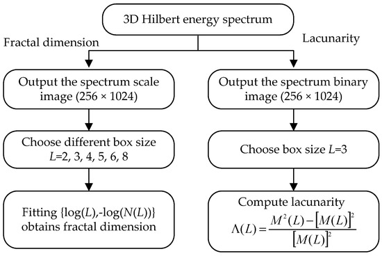
Figure 6.
Procedure for computing fractal dimension and lacunarity.
4.4. Extension Recognition Method
Extension theory contains the concepts of matter-elements and extension sets and its main application is in solving contradiction and incompatibility problems [24]. The matter-element can easily represent the nature of matter, and the extension set is the quantitative tool of the extension theory which represents the correlation degree of the matter-element by the designed correlation function. The membership function of the traditional fuzzy set describes the value of matter at interval [0, 1]. The extension set extends the fuzzy set from [0, 1] to [−∞, ∞]. As a result, it allows for us to define a set that includes any data in the domain [25]. The proposed extension-based recognition method is described as follows.
Step 1: Formulate the matter-element Ri for each defect type as
where
- Ti: the ith defect type of PD pattern,
- Cj: the jth input feature,
- aij: the lower bound of classical domains related to the jth input feature of the ith defect type,
- bij: the upper bound of classical domains related to the jth input feature of the ith defect type.
The classical domain V = <a, b> of each value falls between the lower and the upper bounds on PD records. The neighborhood domain = <f, g> of classical domains, the possible range of each characteristic, can then be determined by setting f = (1 − α) × a and g = (1 + α) × b, where α represents an extend factor. The extension correlation function concept is shown in Figure 7.
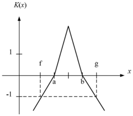
Figure 7.
Extension membership function.
Step 2: Extract the PD features, i.e., the fractal dimension D and the lacunarity Λ, as referred to in Section 4.3.
Step 3: Calculate the degree of the correlation
where
which relates the jth feature of the tested PD pattern to the jth input feature of the ith defect type as in Step 1.
Step 4: Set the weights of respective features W1, W2, W3 In this work, the weights of all features are set equally.
Step 5: Evaluate the correlation index related to each defect type
Step 6: Normalize the correlation index
which falls between [–1, 1] and is seen as a significant quantity for pattern recognition
Step 7: Find the maximum normalized correlation index (or 1). In the case of λk = 1, then the tested model is categorized to the kth defect type. The flow chart of the recognition method based on extension theory is shown in Figure 8.
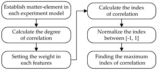
Figure 8.
Flow chart of the extension recognition method.
5. Experiment Results and Discussion
The proposed power cable joints recognition, based on IHHT with fractal feature extraction, was performed based on the electrical signal measured in the experiment models. A total of 240 sets of measurement data were associated with the six types of experiment models. Subsequently, 20 tests are randomly selected for the identification training purpose, while the rest is used for the test purpose. Here, a detected partial discharge signal is analyzed by HHT and IHHT respectively, and various features are extracted out of a time–frequency–energy 3D spectrum, following which the intended defect mode identifications are made using an extension method. A random noise between ±10% to ±30% is introduced into such features to test the ability against noise interference.
5.1. Identification Results by HHT
In this section, a partial discharge signal is analyzed by the conventional HHT, which decomposes extracted IMFs at the same time as signals, since extrema interpolation is adopted during the EMD process. This is an approach well applied to the analysis of a nonlinear as well as non-stationary signal, and the cost is that illusive components are very likely to be evoked. Accordingly, the improved HHT is proposed as an effective approach to enhance the reliability of signal analysis conducted by the conventional HHT. Underpinned by an extension theorem, all the identification processes are made automatic for an easy comparison in terms of identification ratio. Such identification results are about to be discussed in the following section.
Figure 9 is a partial discharge signal, detected on site by an inductive sensor, where the curve in black represents a 60 Hz reference voltage signal, while the one in blue denotes an original partial discharge signal, and demonstrated in Figure 9b is the enlarged portion encircled by the red dash curve in Figure 9a. Subsequently, the field detected signal is analyzed and features contained are extracted by HHT and IHHT respectively. Taking the Hilbert transform of n number of IMFs extracted through an EMD process, a time-frequency-energy spectrum is gained accordingly, due to the reason that it is a superior approach to get the feature extraction done by way of a 3D spectrum rather than by way of a Hilbert spectrum directly.
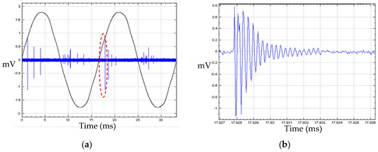
Figure 9.
Partial discharge signal. (a) PD signal in sin wave. (b) One PD pulse.
With the z axis representing the signal energy, presented in Figure 10 are time-frequency-energy 3D spectrums, converted from 10 MHz of Hilbert spectrum as well as a 16 ms time duration, written into a matrix of dimension 256 × 1024. Both the fractal dimension (FD) and lacunarity (Λ) are extracted out of such 3D spectrums, after which the Mean-discharged (M), the 3rd feature, is extracted to plot the distribution as Figure 11. It is noted that there is a significant variation among various feature distributions, but the variation tends to vanish as the effect of mode confusions stemming from illusive components, between similar defect modes, i.e., Types II and III. As tabulated in Table 1, the identification ratio of Type III ranks the lowest place, an evidence that illusive components demonstrate highly negative effect on the identification result.
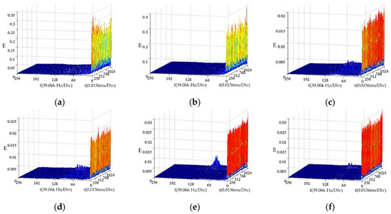
Figure 10.
Time–frequency–energy 3D spectrums by HHT for (a) Type I (b) Type II (c) Type III (d) Type IV (e) Type V (f) Type VI.
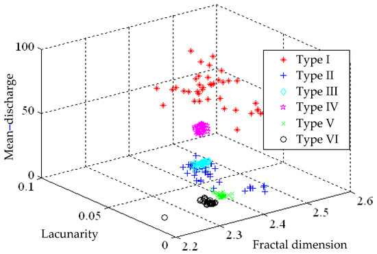
Figure 11.
Feature distributions for time–frequency–energy 3D spectrums by HHT.

Table 1.
Identification results by HHT versus features fractal dimension (FD)- lacunarity (Λ)- mean-discharged (M).
5.2. Identification Results by IHHT
An original detected signal is analyzed here by the IHHT approach as referred to in Section 3. As the first step, the first run of EMD process is performed on such original discharge signal for the purpose of the removal of the trend curve embedded. In the course of the second run of the EMD process, the shifting number remains invariant and the process proceeds until a K-S test result matches the sorting result by signal energy ratio. Subsequently, all the illusive components are ruled out by a cumulative IMF with the highest probability in the proposed IHHT. In the end, time-frequency-energy 3D spectrums are made once again, as demonstrated in Figure 12. As presented in Figure 13, a feature distribution is plotted by way of features, namely fractal dimension and lacunarity, gained by use of an extension theory, and averaged discharged energy. It is seen that the feature distributions, evaluated by IHHT, for Types II, III and IV tend to stay apart from each other, that is, the identification ratio is promoted accordingly. In other words, little difference between similar features can be made more distinguishing through a fractal theory such as the case between Type III and IV. As tabulated in Table 2, the IHHT analysis is demonstrated able to provide an identification ratio up to 50% in the case of Type III. In comparison of 3D spectrums, there is a higher distinction between Types III and IV in Figure 12c,d, the result analyzed by IHHT, than that in Figure 10c,d. In a brief conclusion, the proposed IHHT is an approach able to promote defect mode identification ratios as intended.
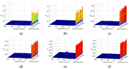
Figure 12.
Time–frequency–energy 3D spectrums by IHHT for (a) Type I (b) Type II (c) Type III (d) Type IV (e) Type V and (f) Type VI.
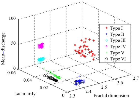
Figure 13.
Feature distributions for time–frequency–energy 3D spectrums by IHHT.
Table 2.
Identification results by IHHT versus features FD-Λ-M.
Even though the identification ratio and the ability against noise interference are improved as a consequence of the removal of illusive components and mode confusions, the identification ratio still remains relatively low between similar defect modes. For this sake, the energy level (E), denoted by the z-axis in the IHHT spectrum, is adopted as the fourth feature. The idea stems from the fact that distinct defect modes represent distinct discharge signals, i.e., various amount of energy is released through insulators. Hence, it is presumed that the adoption of the average energy level as a feature can render a higher identification result. Demonstrated in Figure 14 are the feature distributions of the fractal dimension, lacunarity and average energy, from which it is seen as expected that Type IV exhibits a smaller amount of discharged energy than Type III, simply for the reason that Type IV is designed as an unflawed case, a case supposed to release the minimal amount of discharge energy. As a result, a high distinction is reached in the discharge energy aspect. Tabulated in Table 3 are the identification results based on such four features using an extension method. It is suggested that in the absence of noise interference, an average identification ratio up to 99.2% is reached, a figure superior to that provided by HHT, and the ratio drops to 78.3%, still a satisfactory figure, in the presence of ±30% noise interference.
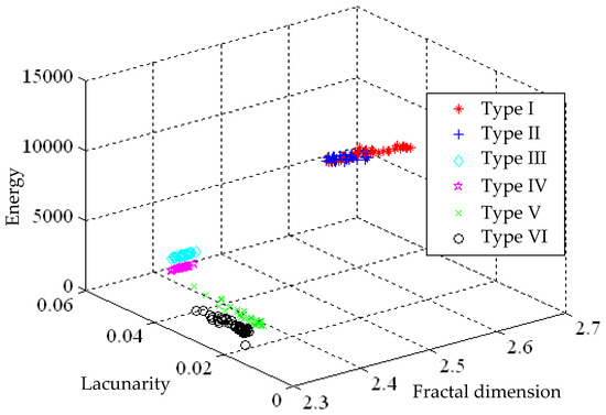
Figure 14.
Feature distributions for time-frequency-energy 3D spectrums by IHHT with the z axis representing the discharged energy level.
Table 3.
Identification results by IHHT versus features FD-Λ-MD-E.
5.3. Identification Results Improved by Phase-Resolved 3D Patterns
For further improving the recognition rates of IHHT, additional PD features extracted from phase-resolved 3D patterns are taken into account. The detailed procedure of feature extraction from a phase-resolved 3D pattern can refer to authors’ previous research [26]. The measured PD field data are first transferred to n-q-φ 3D pattern, and the fractal features and mean-discharge are then extracted from the phase-resolved 3D patterns. Figure 15 shows the typical 3D patterns as transferred from the measured PD data for each experiment model. The parameters of the 3D patterns are number of discharge n, discharge magnitude q, and phase angle φ. We can observe that the amplitude (pC) and numbers of discharge (n) in Type IV and VI are less than the other defect types. In Type I, the discharge amplitude is larger than that in the other defects, the maxima discharge can even reach 350 pC. The experiment Type II and Type V have the similar 3D pattern but discharge amplitude Type V is larger than Type II. According to the 3D PD pattern in each experiment model, we found that the features are different between the defect models. Demonstrated in Figure 16 are the features distributions of the fractal dimension, lacunarity and mean-discharge extract from 3D phase-resolved PD pattern. The patterns belonging to a particular class are close to each other, and the distribution of Type I is very clearly different with other modes. The recognition rates of combining IHHT with phase-resolved n-q-φ 3D PD pattern are shows in Table 4. There are totally seven features as input to extension method for pattern recognition. It can be obviously observed that combining IHHT with phase-resolved PD pattern not only improves recognition rates but also enhances noise tolerance. It can reach 83% even when ±30% noise is added.
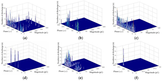
Figure 15.
Phase-resolved 3D patterns for (a) Type I (b) Type II (c) Type III (d) Type IV (e) Type V and (f) Type VI.
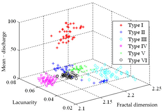
Figure 16.
Feature distributions for phase-resolved n-q-φ 3D pattern.
Table 4.
Identification results improved by combining IHHT with phase-resolved patterns.
As illustrated in Figure 17, a relatively high identification result is provided by IHHT in contrast with HHT as a consequence of the removal of mode confusions, purification of IMFs and features extracted by a fractal theory. Due to the fact that a partial discharge signal is sensed as an extremely weak signal, the marginal difference in 3D spectrums analyzed by both HHT and IHHT is not distinctive enough unless the features are extracted in IHHT by a fractal theorem. This research also combines IHHT with phase-resolved 3D patterns for further improving recognition rates. The results show that more representative features added can effectively raise the recognition rates. However, more complex procedure for both features extraction and pattern recognition are comparatively required.
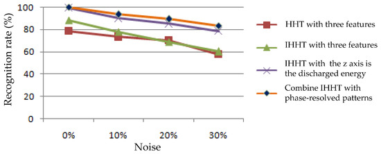
Figure 17.
Mean identification results for various preprocessing approaches.
6. Experiment Results and Discussion
Propose in this work is an improve HHT, which employs a Kolmogorov–Smirnov test and a sorting result by signal energy ratio in the determination of an optimal shifting number. In a bid to rid illusive components, a cumulative K-S test is presented as well, such that all the IMFs can be extracted accurately as expected, the intrinsic physical meaning can be reserved over each spectral band, and then partial mode confusion problems are successfully addressed. This improved HHT approach is then applied to defect mode recognition of partial discharge signals detected from cross-linked polyethylene insulated power cables. It converts the detected discharge signal to a time–frequency–energy 3D spectrum, extracts features, namely fractal dimension, lacunarity and average energy, through a fractal theory, and in the end successfully recognizes defect modes by use of an extension method. By an analysis on a field detected signal, it is concluded that the IHHT combined with phase-resolved PD pattern is demonstrated to be superior to the HTT in terms of identification results and the ability against noise interference.
Acknowledgments
The research was supported by the National Science Council of the Republic of China, under Grant No. MOST 106-2221-E-167-017.
Author Contributions
FengChang Gu a conceived and designed the study; HungCheng Chen performed the experiments in the laboratory; MengHung Chao studied and tested the algorithm; All the coauthors collaborated with respect to the interpretation of the results and in the preparation of the manuscript.
Conflicts of Interest
The authors declare no conflict of interest.
References
- Alvarez, F.; Garnacho, F.; Ortego, J.; Sanchez-Uran, M.A. Application of HFCT and UHF sensors in on-line partial discharge measurements for insulation diagnosis of high voltage equipment. Sensors 2015, 15, 7360–7387. [Google Scholar] [CrossRef] [PubMed]
- Li, P.; Zhou, W.; Yang, S.; Liu, Y.; Tian, Y.; Wang, Y. A novel method for separating and locating multiple partial discharge sources in a Substation. Sensors 2017, 17, 247. [Google Scholar] [CrossRef] [PubMed]
- Wu, K.; Ijichi, T.; Kato, T.; Suzuoki, Y.; Komori, F.; Okamoto, T. Contribution of surface conductivity to the current forms of partial discharges in voids. IEEE Trans. Dielectr. Electr. Insul. 2005, 12, 1116–1124. [Google Scholar]
- Wang, Z.D.; Liu, Q.; Wang, X.; Jarman, P.; Wilson, G. Discussion on possible additions to IEC 60897 and IEC 61294 for insulating liquid tests. IEET Electr. Power Appl. 2011, 5, 486–493. [Google Scholar] [CrossRef]
- Ma, H.; Chan, J.C.; Saha, T.K.; Ekanayake, C. Pattern recognition techniques and their applications for automatic classification of artificial partial discharge sources. IEEE Trans. Dielectr. Electr. Insul. 2013, 20, 468–478. [Google Scholar] [CrossRef]
- Wu, M.; Cao, H.; Cao, J.; Nguyen, H.L.; Gomes, J.B.; Krishnaswamy, S.P. An overview of state-of-the-art partial discharge analysis techniques for condition monitoring. IEEE Electr. Insul. Mag. 2015, 31, 22–35. [Google Scholar] [CrossRef]
- Kreuger, F.H.; Gulski, E.; Krivda, A. Classification of partial discharge. IEEE Trans. Dielectr. Electr. Insul. 1993, 28, 917–931. [Google Scholar] [CrossRef]
- Goldman, M.; Goldman, A.; Gatellet, J. Physical and chemical aspects of partial discharges and their effects on materials. IEE Proc. Sci. Meas. Technol. 1995, 142, 11–16. [Google Scholar] [CrossRef]
- Gulski, E. Digital analysis of partial discharge. IEEE Trans. Dielectr. Electr. Insul. 1995, 2, 822–837. [Google Scholar] [CrossRef]
- Gu, F.C.; Chang, H.C.; Chen, F.H.; Kuo, C.C.; Hsu, C.H. Application of the Hilbert-Huang transform with fractal feature enhancement on partial discharge recognition of power cable joints. IET Sci. Meas. Technol. 2012, 6, 440–448. [Google Scholar] [CrossRef]
- Gu, F.C.; Chang, H.C.; Kuo, C.C. Gas-insulated switchgear PD signal analysis based on Hilbert-Huang transform with fractal parameters enhancement. IEEE Trans. Dielectr. Electr. Insul. 2013, 20, 1049–1055. [Google Scholar]
- Huang, W.; Shen, Z.; Huang, N.E. Use of intrinsic modes in Biology: Examples of indicial response of pulmonary blood pressure to step hypoxia. Proc. Natl. Acad. Sci. USA 1998, 95, 12766–12771. [Google Scholar] [CrossRef] [PubMed]
- Huang, N.E.; Shen, Z.; Long, S.R.; Wu, M.C.; Shih, H.H.; Zheng, Q.; Yen, N.C.; Tung, C.C.; Liu, H.H. The empirical mode decomposition and the Hilbert spectrum for nonlinear and non-stationary time series analysis. Proc. R. Soc. A Math. Phys. Eng. Sci. 1998, 454, 903–995. [Google Scholar] [CrossRef]
- Huang, N.E.; Wu, M.C.; Long, S.R. A confidence limit for the empirical mode decomposition and Hilbert spectral analysis. Proc. R. Soc. 2003, 459, 2317–2345. [Google Scholar] [CrossRef]
- Van, M.; Kang, H.J.; Shin, K.S. Rolling element bearing fault diagnosis based on non-local means de-noising and empirical mode decomposition. IET Sci. Meas. Technol. 2014, 8, 571–578. [Google Scholar] [CrossRef]
- Djuric, P.M.; Miguez, J. Assessment of nonlinear dynamic models by Kolmogorov–Smirnov statistics. IEEE Trans. Signal Process. 2010, 58, 5069–5079. [Google Scholar] [CrossRef]
- Andrade, F.A.; Esat, I.; Badi, M.N.M. A new approach to time-domain vibration condition monitoring: Gear tooth fatigue crack detection and identification by the Kolmogorov-Smirnov test. J. Sound Vib. 2001, 240, 909–919. [Google Scholar] [CrossRef]
- Jackson, R.J.; Wilson, A.; Giesner, D.B. Partial discharges in power-cable joints: Their propagation along a crossbonded circuit and methods for their detection. IEEE Proc. Gener. Transm. Distrib. 1980, 127, 420–429. [Google Scholar] [CrossRef]
- Oyegoke, B.; Birtwhistle, D.; Lyall, J. Condition assessment of XLPE cable insulation using short-time polarisation and depolarisation current measurements. IET Sci. Meas. Technol. 2008, 2, 25–31. [Google Scholar] [CrossRef]
- International Electrotechnical Commission. IEC 60502-2: Power Cables with Extruded Insulation and Their Accessories for Rated Voltages from 1 kV (Um = 1.2 kV) up to 30 kV (Um = 36 kV), Part 2: Cables for Rated Voltages from 6 kV (Um = 7.2 kV) up to 30 kV (Um = 36 kV); International Electrotechnical Commission: Geneva, Switzerland, 1998. [Google Scholar]
- Friesen, W.I.; Mikula, R.J. Fractal dimensions of coal particles. J. Colloid Int. Sci. 1987, 20, 263–271. [Google Scholar] [CrossRef]
- Satish, L.; Zaengl, W.S. Can fractal features be used for recognizing 3-d partial discharge patterns. IEEE Trans. Dielectr. Electr. Insul. 1995, 2, 352–359. [Google Scholar] [CrossRef]
- Mandelbrot, B.B. The Fractal Geometry of Nature; Freeman: New York, NY, USA, 1983. [Google Scholar]
- Cai, W. The extension set and incompatibility problem. J. Sci. Explor. 1983, 1, 81–93. [Google Scholar]
- Wang, M.H.; Ho, C.Y. Application of extension theory to PD pattern recognition in high-voltage current transformers. IEEE Trans. Power Deliv. 2005, 20, 1939–1946. [Google Scholar] [CrossRef]
- Chen, H.C.; Gu, F.C. Pattern recognition with cerebellar model articulation controller and fractal features on partial discharges. Expert Syst. Appl. 2012, 39, 6575–6584. [Google Scholar] [CrossRef]
© 2017 by the authors. Licensee MDPI, Basel, Switzerland. This article is an open access article distributed under the terms and conditions of the Creative Commons Attribution (CC BY) license (http://creativecommons.org/licenses/by/4.0/).