Abstract
The thermo-elastic fracture problem and equations are established for aluminium alloy Metal Inert Gas (MIG) welding, which include a moving heat source and a thermoelasticity equation with the initial and boundary conditions for a plate structure with a crack. The extended finite element method (XFEM) is implemented to solve the thermo-elastic fracture problem of a plate structure with a crack under the effect of a moving heat source. The combination of the experimental measurement and simulation of the welding temperature field is done to verify the model and solution method. The numerical cases of the thermomechanical parameters and stress intensity factors (SIFs) of the plate structure in the welding heating and cooling processes are investigated. The research results provide reference data and an approach for the analysis of the thermomechanical characteristics of the welding process.
1. Introduction
In welding applications, numerical simulation technology is a useful tool for quantitative investigation of various parameters, such as welding temperature, stress, deformations and crack effects. The mathematical model of the welding problem can be simplified as a heat conduction process of a moving point heat source applied on a medium. Li [1] developed a three-dimensional and transient model with a keyhole geometry-dependent heat source and arc pressure distribution for the plasma arc welding process. The dynamic variation of the temperature field and fluid flow in the weld pool were quantitatively analyzed as well as the keyhole shape and size. Zhang [2] investigated the effects of solid-state phase transformation on the residual stress in the welding of Q345 by numerical simulation. He [3] established the temperature field finite element numerical simulation model of twin arc movement; the loading form of the twin arc with a double ellipsoid heat source was discussed; and the laws of molten pool characteristics influenced by the welding speed, current and voltage of the twin-arc submerged arc welding parameters were analyzed. Yaghi [4] conducted finite element simulation of thermal and residual welding stresses in the specific heat of a material. Das [5] developed a model of the heat transfer during welding by the Element Free Galerkin (EFG) method, and demonstrated the effectiveness and utilities of the EFG method for modeling and understanding the heat transfer processes in arc welding. Casalino [6] calculated the temperature distribution and thermal cycle in the workpiece by finite element analysis in dissimilar aluminum titanium laser welding, and he also carried out the finite element method (FEM) study of full penetration keyhole laser welding of Ti6Al4V in butt configuration by varying the modeling strategy of the thermal source [7]. Sheikhi [8] investigated the underlying mechanism involved in the solidification crack in pulsed laser welding of 2024 aluminum alloy experimentally and numerically. He [9] established a three-dimensional welding thermal–mechanical coupling model of aluminum alloy sheet, and analyzed the welding solidification crack tendency by calculation of the welding temperature, stress and the crack driving force curves. The current numerical techniques of welding mainly focus on the non-crack homogeneous or nonhomogeneous structure. In fact, the presence of stress concentration in the material may result in the initiation and extension of a crack in the welding seam zone, which can affect the quality of the structure. However, only few existing models take into account the crack behavior under welding thermal loadings, which are critical to many welding applications, such as automobile, fuel cells and computer components fabrication, etc.
In recent years, the extended finite element method (XFEM) has been the subject of considerable research as a powerful numerical procedure for analysis of the crack problems. Within the framework of thermo-elastic fracture by the XFEM, Duflot [10] investigated the static case of thermo-elastic fracture by XFEM, which considered thermal boundary conditions with different crack faces in both the 2D and 3D problems. Zamani [11] implemented the XFEM to model the effects of mechanical load and thermal shocks on a body with a stationary crack. Bouhala [12] used the extended Element Free Galerkin method (XEFG) to model the crack growth in elastic materials, and investigated the effect of thermo-mechanical loading on the crack growth. Hosseini [13] studied isotropic and orthotropic functionally graded materials (FGMs) under a combination of mechanical and thermal loadings using the XFEM. These implementations of the XFEM for modeling thermo-elastic fracture were successful in the analysis of the thermal crack mechanics, dynamic crack propagation and estimation of the dynamic stress intensity factors (SIFs).
Therefore, the XFEM is implemented to model and solve the thermo-elastic fracture mechanics problem under the welding thermal effect. The temperature, stress and SIFs of the plate structure with a finite crack under a moving heating source are investigated. This paper is organized as follows. In Section 2, we discuss the thermo-elastic fracture problem and equations of the plate with a crack during aluminium alloy Metal Inert Gas (MIG) welding, which include a moving heat source and a thermoelasticity equation with the initial and boundary conditions. In Section 3, the XFEM is implemented to model and solve the thermo-elastic problem of the plate structure with a crack under a moving point source. In Section 4, the SIFs of the thermal crack are introduced. We discuss the calculated results in Section 5. The conclusions are summarized in Section 6.
2. Problem and Equations
2.1. The Moving Heat Source
In numerical modeling of the welding, the Gaussian model of the welding arc is often accepted [9]. The Gauss heat flux distribution function is adopted to achieve moving heat loading in the calculation process, which is in Figure 1.
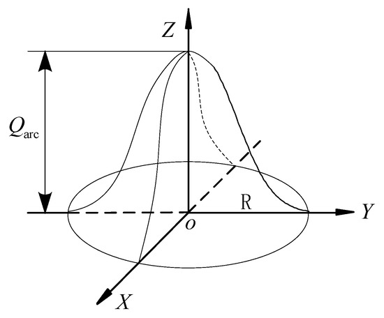
Figure 1.
Schematic of the Gauss heat flux distribution.
The Gaussian distribution model is used to describe the power distribution of the moving heat source of the welding arc, of which the form is as follows
In (1), is the inputting heat of the welding arc, is the thermal efficiency of the welding arc, is the distance between the arbitrary point on the work pieces and the center of the arc, is the effective heating radius of the arc, are the welding arc voltage, current, effecting time and moving speed respectively. The Gauss heat flux distribution is shown in Figure 2.
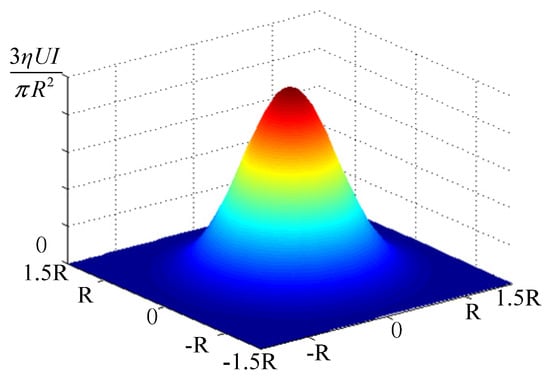
Figure 2.
Gauss heat flux distribution (The colors represent the intensity of the heat flux distribution, the red represents the largest, the blue represents the smallest).
In the practical calculation process [14], the heating flux density are calculated and loaded on the selected node by the Gauss heating source model according to the given welding parameters. The procedure is compiled by the calculation of the new selected node along as the arc moves as follows
2.2. Equations
The problem of instantaneous thermoelasticity of a plate with a crack during welding heating can be represented in Figure 3.
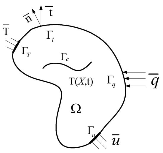
Figure 3.
The thermo-elastic model of the structure caused by a crack during welding heat.
A cracked body with an open initial domain R3 and a piecewise smooth boundary is considered. . represents stress, represents displacement, represents heat flux, represents the stress boundary, represents the displacement boundary, represents the heat flux boundary, represents the temperature boundary. is the transient temperature field throughout the structure produced by the q. q contains a heating source and a heat flux toward the element surface . The problem of instantaneous thermoelasticity consists in the governing equations written by
where the symbol is the spatial gradient operator, is the total density, is the heat source externally into the body per unit volume, is the temperature, is the thermal conductivity of the material. The displacement u, the strain tensor ε, the stress tensor σ and the thermal expansion are defined with respect to a reference temperature ; the material properties are the expansion coefficient and the isotropic fourth-order Hooke tensor D, I is the identity second-order tensor, and is the symmetric gradient operator on a vector field. is the specific heat at constant strain.
The temperature of the structure is at a given time, the prescribed displacements are imposed on , the prescribed stresses are imposed on , is imposed on , is imposed on . The crack forms or propagates, should be accounted as a propagation of the already existing in the body. For this case, the solution for the problem of instantaneous thermoelasticity of the governing Equations (3)–(7) is subjected to the following boundary and initial conditions
where , is the coefficient of heat transfer, is the sink temperature, is the value of absolute zero of the temperature scale. is the radiation coefficient.
3. The XFEM Formulation of Governing Equations
The XFEM is employed to numerically model an elasticity medium with discontinuities by adding appropriate enrichment functions to the standard finite element (FE) approximation. In order to derive the weak form of the governing Equations (3) and (4), the trial functions , and the test functions , are required to be smooth enough to satisfy all essential boundary conditions. To obtain the weak form of the governing equations, the test functions and are multiplied by Equations (3) and (4) respectively, and integrated over the domain as
Applying the Divergence theorem, the following weak form of the governing equations is obtained by expanding the integral Equations (14) and (15).
It must be noted that the total stress in the integral (16) must be replaced by Equation (6), which is written as follows.
The spatial and time domain discretization of the integral Equations (16) and (17) are derived using the XFEM and generalized Newmark approaches.
3.1. Approximation of Displacement and Temperature Fields
The discrete form of the integral Equations (16) and (17) can be obtained in the XFEM using the test and trial functions for the displacement and temperature fields. The trial functions are defined as follows [15].
The variables are the additional degree of freedom (DOF) according to enrichment functions. is the standard shape functions of displacement fields. is the additional asymptotic enrichment functions depending on the tip singularity of the displacement or temperature field. is the Heaviside step function.
The discretization of (17) in terms of the temperature is similar to Equation (16). The main difference is the number of the branch functions. The other difference is the introduction of the temperature as body forces [12]. The trial functions can be defined as follows.
The variables and are the additional DOF according to enrichment functions. are the standard shape functions of displacement and temperature fields. It is noted that is different in the case of an adiabatic or an isothermal crack analysis.
(1) Adiabatic crack
The adiabatic crack is defined by a zero flux normal to the crack surface that causes a discontinuity in the temperature field. Therefore, the signed distance function is used as an enrichment function in this case [12], since it ensures the discontinuity of the temperature and the continuity of its derivative through the crack.
The tip nodes are enriched by the branch function that is given by
(2) Isothermal crack
The crack is considered as isothermal when the temperature has a constant value on the crack surface, which causes a discontinuous heat flux with the continuous temperature field. The enrichment function that can satisfy these conditions is the one proposed by Moës et al. [16].
The near tip nodes are enriched by
The enriched FE approximation of the displacement (19) and temperature (20) can be symbolically written in the following form.
is the matrix of the standard displacement shape functions. and are the matrices of the enriched displacement shape functions associated with the Heaviside and asymptotic tip functions. is the matrix of the standard temperature shape functions, and and are the matrices of the enriched temperature shape functions associated with the Heaviside and asymptotic tip functions.
3.2. The XFEM Spatial and Time Discretization
Applying the trial and the test functions, the discretized forms of integral Equations (16) and (17) can be obtained according to the Bubnov–Galerkin technique as follows.
where and are the complete set of the standard and enriched DOF of the displacement and temperature fields respectively. The matrices K, W, R, C and external force vectors f and g are defined as follows.
and
where denote the “standard”, “Heaviside”, and “asymptotic tip” functions of the displacement field. denote the “standard”, “Heaviside”, and “asymptotic tip” functions of the temperature field. In these definitions, m is the vector of the delta Dirac function defined as .
In order to complete the numerical solution of XFEM equations, it is necessary to integrate the differential Equation (27) in time. The Newmark method is used for the elastic part of the problem [15,17]. Meanwhile, in the numerical integration of the XFEM formulations, the crack discontinuity must be properly taken into account when the integration is performed, or this may lead to poor numerical results. So, the crack discontinuity must be taken as an internal boundary of the domain of the element, and the integration must be carried out by dividing the domain of the element into two sub-domains to perform the integration on these two sub-domains. The XFEM formulations involve the discontinuity along the crack and the singularity at the crack tip. In order to implement the standard integration method in the XFEM formulation, the element cut by the crack surface must be first divided into several sub-polygons, and the numerical integration is then performed over each sub-polygon. The numerical integration method of discontinuity is shown in Figure 4, in which the crack does not coincide with the rectangular edges that cause some approximation in the numerical simulation [15]. The discontinuity is divided into sub-triangles. It must be noted that more triangular sub-divisions are necessary in the tip element.
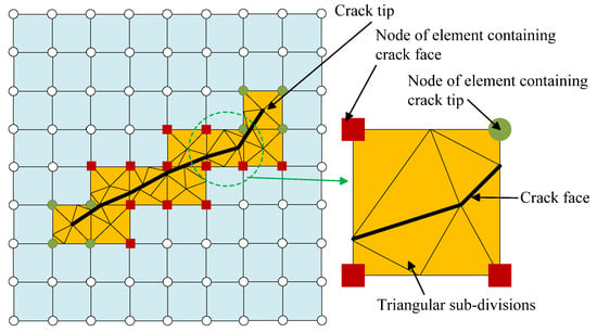
Figure 4.
The triangular sub-divisions scheme of the numerical integration of crack discontinuity in the extended finite element method (XFEM).
4. Stress Intensity Factors (SIFs)
The SIFs are extracted from the XFEM solution with the help of the crack tip path-independent integrals, which have been extended to the thermal crack problems [10,11,12,15]. The interaction integral method is applied to calculate the SIFs [18]. The J integral over a path around the crack tip is defined as (see Figure 5)
is the mechanical strain energy density defined as
denotes the stress tensor, is the displacement field, is the unit outward normal vector to the contour integral , is the Kronecker delta, and is the traction on the contour integral .
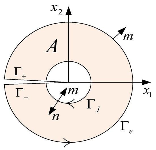
Figure 5.
J integral contour around the crack tip.
In order to establish a domain form of the integral that is suitable for the extraction of the SIFs from a numerical solution, a second path surrounding is considered and the region A between and is defined. The region A is bounded by + + + where and are paths located on each of the crack faces. Equation (30) can be recast into
where m is the outward normal to A. q is a weighting function defined over the domain of integration. The crack faces are assumed to be traction free. Applying the divergence theorem to Equation (32) and using the equilibrium and strain-displacement equations, the domain form of the J integral is then obtained by
where is the expansion coefficient. Two states of a cracked body are considered. The interaction integral is formulated by superimposing the actual and auxiliary fields on the path independent J-integral. State one corresponds to the actual fields. State two is an auxiliary field which will be chosen as the asymptotic field for modes I, II or III. The J-integral for the sum of the two states can be written as
where is called the interaction integral between states one and two.
The auxiliary fields are independent of the thermal loading, they are exactly the same as in non-thermoelasticity. The interaction integral is obtained as
From the second term of the integrand of Equation (35), the thermal loading has a similar effect in the interaction integrals between the actual fields and some auxiliary fields, which is suitable for the extraction of the individual SIFs.
For general mixed-mode loading, the part of the crack inside is straight, it is independent of the path, and the value of the J-integral related to SIFs is obtained as
If the auxiliary state is assumed as the pure mode I asymptotic fields, that is, and , the SIFs of mode I can be stated as
In a similar way, mode II and mode III SIFs can be obtained from the value of the interaction integral.
5. Numerical Results and Discussion
5.1. Simulation and Experimental Verification
In welding numerical simulation, the heat transfer in the workpiece and around the surrounding environment should be considered, which is shown in Figure 6. The source of the arc inputs a large amount of heat into the workpiece in the heating process, which rises temperature rapidly in the welding seam zone. In the heating process, the heat transfers from the center zone of the workpiece to the lower temperature zone, which inevitably causes changes within the metal microstructure due to the thermal expansion effect. The heating effect from the source of the arc is over in the cooling process, the heat transfer between the workpiece and the surrounding environment is continuing, the temperature of the workpiece gradually becomes lower, with cooling contraction in the metal microstructure. In both the processes, the thermal crack may initiate or change dynamically in the welding seam zone over which the moving heat source moves. Therefore, the heating and cooling processes are necessarily considered to calculate the temperature field, displacement field and the dynamic response in the welding workpiece.
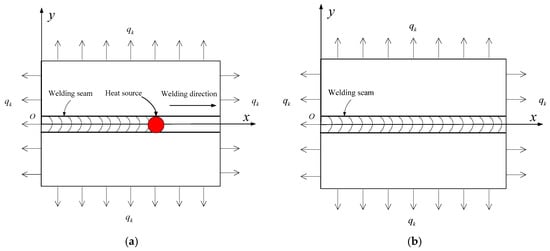
Figure 6.
The geometry and welding heating and cooling processes, (a) heating process; (b) cooling process.
The finite element model of the thin plate hardfacing welding is adopted to be simulated and analyzed. The welding material is 2024 aluminum alloy, the welding geometry size is 80 mm × 60 mm × 2 mm, the welding joint is located in the center line of the x–y plane and the arc center moves along the x axis with a speed of v = 2 mm/s.
In numerical calculations, the heat source model (3) is used with the thermal efficiency η = 0.9, the effective heating radius of the arc R = 3.0 mm, the welding voltage U = 20 V, the welding current I = 160 A, the welding speed v = 2 mm/s. The calculation times of the heating and cooling processes are 40 and 140 s respectively. The coefficient of the heat transfer ak = 50 W/(m2·K), ϑ = ε × Φ, ε is the radiation coefficient with the value of 0.5; Φ is the Stefan Boltzmann constant with the value of 5.670373 × 10⁻⁸ kg·s−3·K−4.
Material properties’ parameters include the thermal conductivity coefficient λ (W/(m·°C)), density ρ (Kg/m3), specific heat c (J/(Kg·°C)), coefficient of thermal expansion α (°C−1) and elastic modulus E (GPa). The material parameters can be treated as a function of temperature with isotropic property. Initial temperature of aluminum alloy sheet is chosen by 20 °C; the material performance parameters at different temperatures are shown in Table 1; the data that are more than 400 °C in Table 1 are obtained by the extrapolation method.

Table 1.
Material properties.
The linear elastic stress–strain relation is not satisfied when the temperature of the material is heated above the melt temperature. In the welding process, when the temperatures of the elements in the XFEM model exceed the upper limit temperature value of the solid–liquid zone, the elements are not involved in the calculation of the thermal stress in the welding process. When the temperatures of the elements are lower than the upper limit temperature value of the solid–liquid zone, the elements are involved in the calculation of the thermal stress in the welding process.
The first example is of a plate without an isothermal crack in the heating and cooling processes. The distributions of the temperature at different times in the heating process are shown in Figure 7. The distributions of the temperature at different times in the cooling process are shown in Figure 8.
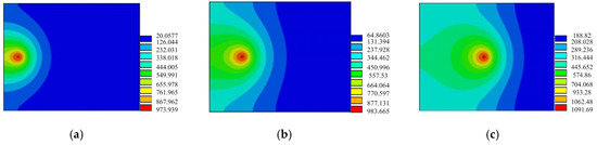
Figure 7.
Temperature contour of the plane without cracks in the heating process (0 < t < 40 s). (a) t = 5 s; (b) t = 10 s; (c) t = 18 s.
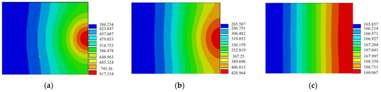
Figure 8.
Temperature contour of the plane without cracks in the cooling process (40 < t < 180 s). (a) t = 50 s; (b) t = 80 s; (c) t = 100 s.
Figure 7 and Figure 8 represent the temperature distribution of aluminum alloy plate in the welding heating and cooling processes. It can be seen that the high temperature area mainly concentrates on the welding center area; the highest temperature zone moves as the heat source. The heating quantity diffuses to the heating affected zone, of which the temperature of the workpiece tends to be balanced. The calculated results are in good agreement with the existing ones. In addition, it can be seen that the heat conduction on the workpiece is continuous, and the temperature gradient is distributed in the welding heating and cooling processes.
In order to validate the effectiveness of the proposed method, the real-time temperature curve of the weldment surface is measured by the infrared thermal imager in the welding experiment [9,19], which is shown in Figure 9.
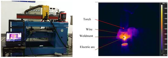
Figure 9.
The temperature measured by the experiment.
The plate surfacing MIG welding experiment of 2024 aluminum alloy sheet is done. The testing is carried out by the infrared thermal imaging instrument. The size of the base material is 80 mm × 60 mm × 2 mm. The three measuring points of the welding plate surface are measured by the infrared thermal imaging instrument, the layout of which is shown in Figure 10.
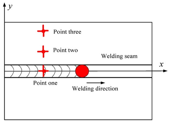
Figure 10.
Temperature measuring point distribution.
The thermal cycle curve of the three measuring points is obtained, which is shown in Figure 11. It can be seen that the temperatures of the three measuring points rise rapidly as the welding heating source moves along the center zone of the workpiece. It reaches the maximum value in a very short time. Then, the temperature of each point descends slowly to be a value. The temperature rising rate of each point is higher than the falling one in the cooling process. In the welding heating process, the temperature of the welding seam zone is much greater than that of the heat affected zone. The maximum temperature value of point one is higher than that of the other points. The temperature of each point tends to be uniform as time goes on in the cooling process, which is consistent with the welding temperature field characteristics.
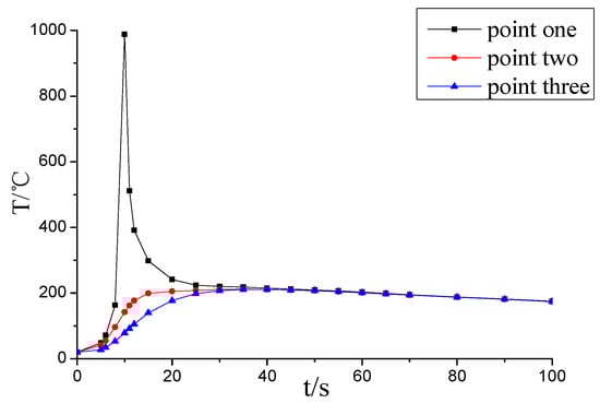
Figure 11.
Thermal cycle curves of the experiment.
The effective heating radius of the Gauss heat source is adjusted to meet the agreement between the simulation and experiments [9]. The effective heating radius of the Gauss heat source is determined by an infrared thermal imaging temperature measurement experiment [9,19]. The appropriate radius is 4.0 mm corresponding to the welding parameters of I = 160 A, voltage U = 20 V and speed v = 2 mm/s. Figure 12 is the comparison of thermal cycle curves of the calculation and experiment at point one. The results show that the simulation results are close to the experimental results.
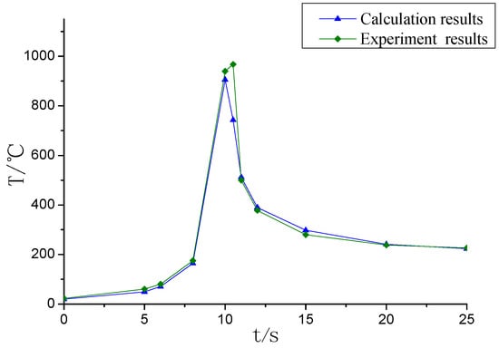
Figure 12.
Comparison of thermal cycle curves of the calculation and experiment at point one.
5.2. The Welding Temperature and Stress Field of Aluminum Alloy Plate with an Isothermal Crack
The welding temperature and stress field of aluminum alloy plate with an isothermal crack are calculated using the indirect coupling method. The stress field is obtained by loading a predefined temperature field, which is divided into the heating and cooling processes. The heating process time is 40 s with 150 incremental steps. The cooling process time is 140 s with 200 incremental steps.
5.2.1. The Welding Temperature and Stress Field Distribution
The geometry and boundary conditions of the heating process are shown in Figure 13; the geometry of the model is 80 mm × 60 mm × 2 mm. The crack is formed in the welding seam zone where the moving heating source has moved at a moment in the welding process. The isothermal crack is predefined with the length of 8 mm (the crack area is between x = 16 to x = 24 with y = 0).
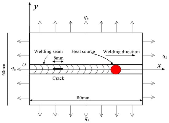
Figure 13.
Geometry and boundary condition of the welding heating process with an inclined isothermal crack.
The distributions of the temperature, heat flux and stress of the plate with an inclined isothermal crack at time of 30 s in the heating process are shown in Figure 14.
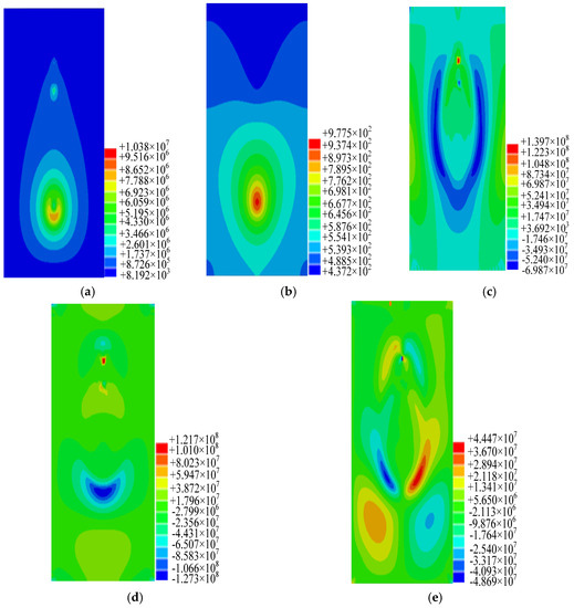
Figure 14.
A plate with an inclined isothermal crack at the heating process: (a) the distribution of heat flux; (b) the distribution of temperature; (c) the distribution of stress σx; (d) the distribution of stress σy; (e) the distribution of stress σxy.
The geometry and boundary conditions of the cooling process are shown in Figure 15. The distributions of the temperature, heat flux and stress of the plate with an inclined isothermal crack at a time of 40 s in the cooling process are shown in Figure 16.
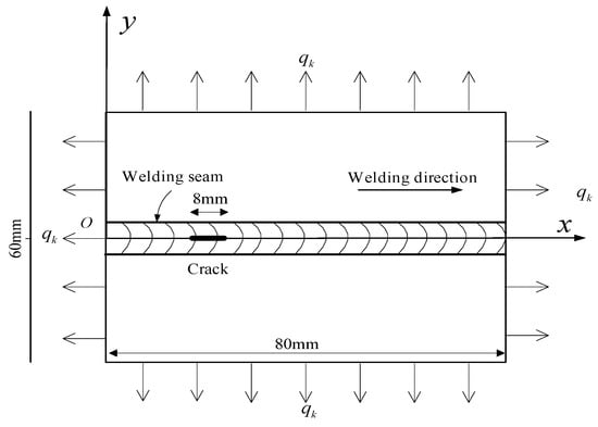
Figure 15.
Geometry and boundary conditions of the welding cooling process with an inclined isothermal crack.
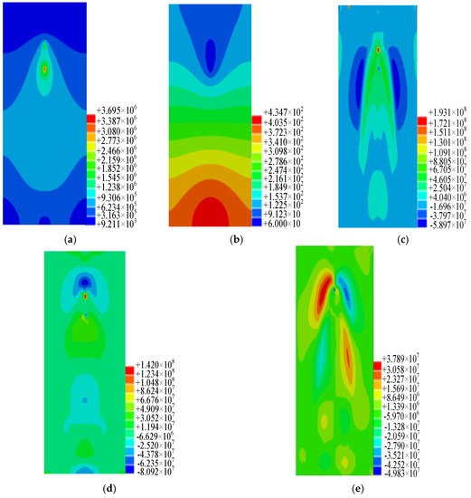
Figure 16.
A plate with an inclined isothermal crack at the cooling process: (a) the distribution of heat flux; (b) the distribution of temperature; (c) the distribution of stress σx; (d) the distribution of stress σy; (e) the distribution of stress σxy.
It can be seen that the temperature and heat flux distribution are symmetrical along the welding seam. The temperature value in the heat source is maximum, and the crack tip along the welding direction appears heat flow concentration. The temperature of the crack in the heating and cooling processes is much lower than those of other regions; the reason is that with the isothermal crack with the initial temperature of a low constant value, the heat dissipation of the crack is fast with high heat flux. The distributions of stress σx and σy on the area away from crack are symmetrical along the welding seam; distribution of stress σxy is asymmetric. The two-crack tip appears as stress concentration; the reason is that the welding area near the crack has great thermal stress in the heating and cooling processes.
The calculation results of the welding temperature and heat flux field distribution are in good agreement with the actual results. At the same time, it is found that the temperature and heat flux distribution are disturbed by the discontinuity of the crack. The heating flow field near the crack tip is obviously concentrated. In the welding heating and cooling processes, the stress gradient near the crack tip is more obvious, and there is obvious stress concentration at the crack tip.
5.2.2. Stress and Strain Field near the Crack in the Welding Heating and Cooling Processes
The geometry and boundary conditions of the heating process are also shown in Figure 13. The crack is formed in the welding seam zone at a time of 12 s in the welding process. The isothermal crack is predefined with the length of 8 mm (the crack area is between x = 16 to x = 24 with y = 0). The stress field near the crack tip is observed as beginning from a welding heating time of 12 s. Figure 17 is the element distribution of the stress field near the crack tip for observation. Eight elements near the crack tip stress are selected to be drawn as a curve. Figure 18 is the time history curve of the stress of the eight elements that began from a welding heating time of 12 s. The values and general trends of stress at different times can be mastered by observation of Figure 18.
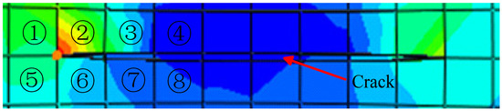
Figure 17.
Element distribution of the stress field near the crack tip for observation (The colors represent the intensity of the stress field, the red represents the largest, the blue represents the smallest).
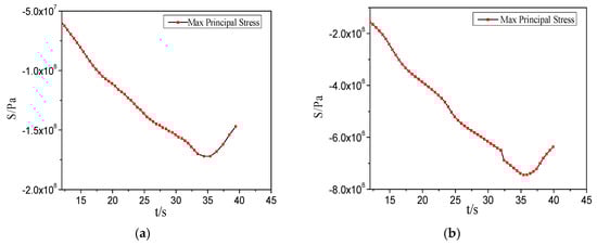
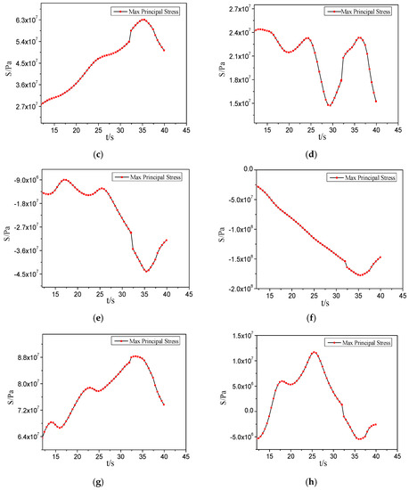
Figure 18.
The stress curves of the elements near the crack tip in the heating process. (a) The stress curve of element ①; (b) The stress curve of element ②; (c) The stress curve of element ③; (d) The stress curve of element ④; (e) The stress curve of element ⑤; (f) The stress curve of element ⑥; (g) The stress curve of element ⑦; (h) The stress curve of element ⑧.
It can be seen from Figure 18 that the stresses of elements ①, ②, ⑤ and ⑥ are all linear in growth and obvious stress concentration. The reason is that the crack tip is affected by the thermal expansion and hampered by the nearby area of metal. The crack tip affected by the temperature becomes weak as the welding heat source moves far away from the crack. The stress values fall back at the end of welding. The stress values of elements ③, ④, ⑦ and ⑧ fluctuate obviously compared to that of elements ①, ②, ⑤ and ⑥. The maximum principal stress values of elements ④, ⑤, ⑦ and ⑧ fluctuate significantly. The reason is that the heat flux distribution is interfered by the discontinuity of the crack, which causes the fluctuations of the temperature and the stress value.
Figure 19 is the time history curves of stress of the eight elements in the welding cooling process. The changing conditions of stress of the eight elements in the welding cooling process can be observed in Figure 19.
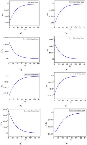
Figure 19.
The stress curves of the elements near the crack tip in the cooling process. (a) The stress curve of element one (b) The stress curve of element two; (c) The stress curve of element three; (d) The stress curve of element four; (e) The stress curve of element five; (f) The stress curve of element six; (g) The stress curve of element seven; (h) The stress curve of element eight.
It can be seen from Figure 19 that the stress of the elements near the crack tip all decrease rapidly as the cooling progresses. The reason is that the strong transient cooling effect is produced when the welding heat source suddenly disappears at the beginning of cooling. The cooling rate of the welding seam zone is the fastest. The stress value of the welding seam zone is changed rapidly. The decreasing rate of stress becomes slow after cooling in a period of time. The cooling rate becomes lower as the temperature difference becomes small. The welding stress value decreases slowly as the temperature becomes low. The final stress value is not zero when the cooling is over, at which point the final residual stress exists.
5.3. Calculation and Analysis of SIFs
The SIFs indicate the cracking tip state extent in the form of a numerical value, which can characterize the strength of the stress and strain field near the crack tip. The SIFs are determined by the size of the external force, loading mode, crack size and shape, and the geometry and size of the work pieces. The SIFs in the heating and cooling processes are obtained by the XFEM. The SIFs of the crack are shown in Figure 20 and Figure 21.
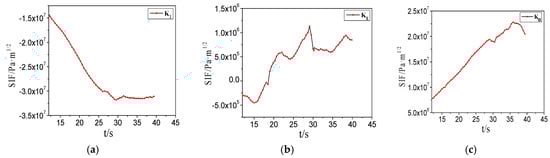
Figure 20.
The stress intensity factors (SIFs) of the crack in the heating process. (a) KI; (b) KII; (c) KIII.
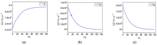
Figure 21.
The stress intensity factors (SIFs) of the crack in the cooling process. (a) KI; (b) KII; (c) KIII.
It can be seen from Figure 20 that the absolute value of KI is almost linear in growth in the welding heating process. The KI value is negative because the obvious stress exists when the welding heating expansion of the crack tip is hampered by the nearby area metal. The value of KII firstly has a small and slow decrease, then appears to fluctuate and has a tendency to decrease after reaching the maximum. The value of KIII is basic linear growth at the beginning of the welding; the value becomes larger as the distance between the heating source and the crack tip becomes far. The value of KIII begins to decrease when the welding is over.
It indicates that the SIFs are changed under the effect of the moving heating source. Three types of SIFs reach the maximum and the minimum value in the heating process with different variation trends.
It can be seen from Figure 21 that the KI, KII and KIII all tend to be a certain value in the welding cooling process. The reason is that the welding heating stress of the crack tip is reduced when the effect of the moving heating source disappears. However, the three types of SIFs are not reduced to zero, because there still exists a certain value of welding residual stress after the welding cooling. Due to an obvious temperature gradient caused by the moving heating source, the values of KI, KII and KIII do not form a very smooth curve, which is due to the slight fluctuation. The SIFs of the crack are all gradually stabilized when the temperature of the workpiece tends to be balanced.
6. Conclusions
In this study, the thermo-elastic fracture problem and equations have been established aluminium alloy MIG welding. The heating source is Gauss heat flux distribution. The XFEM is successfully implemented to solve the thermo-elastic fracture problem of a plate structure with a crack during the heating and cooling processes. The numerical cases of the temperature, stress and SIFs of the plate structure with a finite crack under the welding heating and cooling processes are investigated and discussed. The calculated welding temperature results are in good agreement with the existing literature. The temperature, heat flux and stress distribution calculated by the XFEM are interfered with by the crack with obvious concentration. The SIFs are changed by the effect of the temperature field in the heating and cooling processes. The SIFs are all gradually stabilized when the temperature of the workpiece tends to be balanced. This study provides an effective method to implement the welding thermal elastic mechanics calculation of aluminum alloy plate with a crack. Further work will focus on the following two aspects and provide reference for the suppression of a hot crack in aluminum alloy MIG welding. The parameters and the effective heating radius of the Gauss heat source model under different welding parameters are determined. Combined with a stress testing experiment, the temperature and stress distribution under different welding parameters are calculated and analyzed to master the changing rules and characteristics of aluminum alloy MIG welding. For the SIFs of different crack locations, further analyses under different welding parameters are conducted to master the dynamic behavior of the crack in aluminum alloy MIG welding.
Acknowledgments
This work is supported by National Natural Science Foundation of China (51475159) and Hunan Provincial Natural Science Foundation of China, are gratefully acknowledged.
Author Contributions
Kuanfang He set up the theoretical model and wrote the paper; Qing Yang performed the calculation and designed the experiments, Dongming Xiao analyzed the data and performed the experiments, Xuejun Li contributed the materials and analysis tools.
Conflicts of Interest
The authors declare no conflict of interest.
References
- Li, T.Q.; Wu, C.S. Numerical simulation of plasma arc welding with keyhole-dependent heat source and arc pressure distribution. Int. J. Adv. Manuf. Technol. 2015, 78, 593–602. [Google Scholar] [CrossRef]
- Zhang, H.; Wang, D.P.; Li, S. Numerical simulation of welding residual stress considering phase transformation effects. Adv. Mater. Res. 2011, 295–297, 1905–1910. [Google Scholar] [CrossRef]
- He, K.; Chen, J.; Xiao, S. Numerical simulation for shaping feature of molten pool in twin-arc submerged arc welding. Open J. Appl. Sci. 2012, 2, 47–53. [Google Scholar] [CrossRef]
- Yaghi, A.H.; Hyde, T.H.; Becker, A.A.; Sun, W. Finite element simulation of welding and residual stresses in a P91 steel pipe incorporating solid-state phase transformation and post-weld heat treatment. J. Strain Anal. Eng. Des. 2008, 43, 275–293. [Google Scholar] [CrossRef]
- Das, I.R.; Bhattacharjee, K.S.; Rao, S. Welding heat transfer analysis using Element Free Galerkin method. Adv. Mater. Res. 2011, 410, 298–301. [Google Scholar] [CrossRef]
- Casalino, G.; Mortello, M. Modeling and experimental analysis of fiber laser offset welding of Al-Ti butt joints. Int. J. Adv. Manuf. Technol. 2016, 83, 89–98. [Google Scholar] [CrossRef]
- Casalino, G.; Mortello, M. A FEM model to study the fiber laser welding of Ti6Al4V thin sheets. Int. J. Adv. Manuf. Technol. 2016, 86, 1339–1346. [Google Scholar] [CrossRef]
- Sheikhi, M.; Ghaini, F.M.; Assadi, H. Solidification crack initiation and propagation in pulsed laser welding of wrought heat treatable aluminum alloy. Sci. Technol. Weld. Join. 2014, 19, 250–254. [Google Scholar] [CrossRef]
- He, K.F.; Zhang, Z.J.; Tan, Z.; Cheng, Y. Thermodynamic characteristics analysis of aluminium welding process. Mater. Res. Innov. 2015, 19, 89–93. [Google Scholar] [CrossRef]
- Duflot, M. The extended finite element method in thermoelastic fracture mechanics. Int. J. Numer. Methods Eng. 2008, 74, 827–847. [Google Scholar] [CrossRef]
- Zamani, A.; Eslami, M.R. Implementation of the extended finite element method for dynamic thermoelastic fracture initiation. Int. J. Solids Struct. 2010, 47, 1392–1404. [Google Scholar] [CrossRef]
- Bouhala, L.; Makradi, A.; Belouettar, S. Thermal and thermo-mechanical influence on crack propagation using an extended mesh free method. Eng. Fract. Mech. 2012, 88, 35–48. [Google Scholar] [CrossRef]
- Hosseini, S.S.; Bayesteh, H.; Mohammadi, S. Thermo-mechanical XFEM crack propagation analysis of functionally graded materials. Mater. Sci. Eng. A 2013, 561, 285–302. [Google Scholar] [CrossRef]
- Piekarska, W.; Kubiak, M.; Saternus, Z. Application of Abaqus to analysis of the temperature field in elements heated by moving heat sources. Arch. Foundry Eng. 2010, 10, 177–182. [Google Scholar]
- Khoei, A.R. Extended Finite Element Method: Theory and Applications; John Wiley & Sons Inc.: Hoboken, NJ, USA, 2015; pp. 1–565. [Google Scholar]
- Gravouil, A.; Moës, N.; Belytschko, T. Non-planar 3D crack growth by the extended finite element and level sets-Part II: Level set update. Int. J. Numer. Methods Eng. 2002, 53, 2569–2586. [Google Scholar] [CrossRef]
- Liu, Z.; Oswaldb, J.; Belytschkoa, T. XFEM modeling of ultrasonic wave propagation in polymer matrix particulate fibrous composites. Wave Motion 2013, 50, 389–401. [Google Scholar] [CrossRef]
- Moran, B.; Shih, C.F. A general treatment of crack tip contour integrals. Int. J. Fract. 1987, 35, 295–310. [Google Scholar] [CrossRef]
- Campanelli, S.L.; Casalino, G. Analysis and comparison of friction stir welding and laser assisted friction stir welding of aluminum alloy. Materials 2013, 6, 5923–5941. [Google Scholar] [CrossRef]
© 2017 by the authors; licensee MDPI, Basel, Switzerland. This article is an open access article distributed under the terms and conditions of the Creative Commons Attribution (CC-BY) license (http://creativecommons.org/licenses/by/4.0/).