Article

A Genetic Regulatory Network-Based Method for Dynamic Hybrid Flow Shop Scheduling with Uncertain Processing Times

School of Mechanical Engineering, Shanghai Jiao Tong University, Shanghai 200240, China
*
Author to whom correspondence should be addressed.
Appl. Sci. 2017, 7(1), 23; https://doi.org/10.3390/app7010023
Submission received: 2 November 2016 / Revised: 6 December 2016 / Accepted: 19 December 2016 / Published: 4 January 2017
(This article belongs to the Special Issue Modeling, Simulation, Operation and Control of Discrete Event Systems)

Abstract

:
The hybrid flow shop is a typical discrete manufacturing system. A novel method is proposed to solve the shop scheduling problem featured with uncertain processing times. The rolling horizon strategy is adopted to evaluate the difference between a predictive plan and the actual production process in terms of job delivery time. The genetic regulatory network-based rescheduling algorithm revises the remaining plan if the difference is beyond a specific tolerance. In this algorithm, decision variables within the rolling horizon are represented by genes in the network. The constraints and certain rescheduling rules are described by regulation equations between genes. The rescheduling solutions are generated from expression procedures of gene states, in which the regulation equations convert some genes to the expressed state and determine decision variable values according to gene states. Based on above representations, the objective of minimizing makespan is realized by optimizing regulatory parameters in regulation equations. The effectiveness of this network-based method over other ones is demonstrated through a series of benchmark tests and an application case collected from a printed circuit board assembly shop.

Graphical Abstract

1. Introduction

The Hybrid Flow Shop (HFS) is a typical discrete manufacturing system in which a set of jobs passes through a series of production stages to complete required operations. The stages are composed of parallel machines to protect the job flow from being blocked by a single machine [1,2,3]. The operation processing time varies with different machines because capacities of parallel machines are normally unrelated at each stage [4,5]. This type of workshop exists in various industries, which include Printed Circuit Board (PCB) assembly, textile production and automobile assembly [6,7,8,9].
Since the first HFS problem was described by Salvador [10], vast amounts of academic work have been carried out on HFS scheduling due to its complexity and practical relevance [11,12,13,14,15]. Different kinds of methods (e.g., exact methods, heuristics and metaheuristics) were proposed to minimize a variety of objectives, which include the maximum completion time, the maximum flow time, the number of late jobs [16,17,18,19]. In terms of minimizing the maximum completion time, i.e., makespan, Mirsanei et al. [20] proposed a simulated annealing algorithm to solve the HFS scheduling problem featured with sequence-dependent setup times. Wang et al. [21] developed an efficient dispatching rule together with several local search heuristics in a semiconductor manufacturing system. Wang et al. [22] proposed a branch-and-bound algorithm to investigate the two-stage HFS scheduling problem in a no-wait environment. Komaki et al. [23] developed several algorithms featured with a new lower bound to minimize the makespan in a specific HFS consisting of two machining stages and one assembly stage.
In most of these approaches, the processing times were assumed to be deterministic in HFS scheduling. However, in a real workshop, the differences between machines, worker skill levels and material qualities make the processing times constantly changing [24]. These variations might lead to increased objective values during the execution of predetermined plans, which occurs frequently in practical production [25,26]. To deal with this situation, dynamic scheduling used for HFS scheduling problems consists of three major ways: proactive, reactive and predictive-reactive [27,28].
The proactive scheduling strategy focuses on generating a robust solution that satisfies performance requirements predictably [29]. This strategy normally uses fuzzy theory or statistical analysis to construct the probability distribution of processing times and applies these distributions to HFS scheduling [30,31]. Nevertheless, it is difficult to ensure the predicted performance in practical situations. In a reactive scheduling strategy, all the decisions are made in real time to react rapidly to dynamic events of processing time uncertainty, e.g., by using dispatching rules and game theory approaches [32,33,34]. However, this strategy can hardly ensure the global performance of HFS scheduling because of the limits placed on computational burden in real-time scheduling. Predictive-reactive scheduling generates a predictive plan based on an expected production environment and revises the plan if dynamic events cause the actual situation differs from expectation [35,36]. This strategy has been widely used because it can achieve a good balance between global performance of solutions and in-time reaction to unexpected situations.
In a predictive-reactive scheduling, predetermined plans are revised by rescheduling in a rolling horizon, rather than in the whole horizon, in order to avoid too much computational efforts [37]. Three types of rolling horizon rescheduling mechanisms, including cycle-driven rescheduling, event-driven rescheduling and mixed driven rescheduling, are developed as an alternative. Of these mechanisms, the event-driven one is most widely used because it can respond to event-related disturbances in a real time. In this mechanism, the reactive scheduling is normally motivated by disturbances beyond a specific level in order to reduce the rescheduling for frequently occurring events.
However, it is currently challenging to find out a method that can achieve a good balance between solution quality as well as computational time when it is necessary to consider rescheduling in HFSs. Heuristic methods obtain a feasible solution quickly, but can hardly ensure the solution quality because they fail to take all the aspects of HFS scheduling into account. Alternatively, metaheuristic methods are capable of finding out optimal solutions owing to their general procedures. Nevertheless, these procedures require too much computational effort and will make the rescheduling plan not a real-time one. Consequently, it is necessary to develop an efficient rescheduling method for the dynamic scheduling of HFS.
The Genetic Regulatory Network (GRN) is a structured network that describes the regulation of gene expression in cells [38]. It has been attracting increased attention because of its excellent description capacity, and various methods, including directed graphs, Boolean networks, rule-based formalisms, qualitative differential equations, Bayesian networks and partial differential equations are currently alternative to construct such a network [39]. A GRN has at least the following three elements in common: genes, gene regulations and gene expression procedures [40]. Each gene has two alternative states (i.e., the expressed state and the unexpressed state). If a gene is in the expressed state, it has inhibitory effects on the states of other ones, which is the primary form of gene regulations. Based upon these regulations, the gene expression procedure converts iteratively certain genes in the unexpressed state into ones in the expressed state if there are few inhibitory effects on these genes. According to genes in the expressed state, the GRN finally determines a specific morphology for the related cell. For instance, Figure 1 illustrates a GRN composed of three genes and constructed by differential equations. In this network, μz (z = 1–3) represents the state of gene z; σz (z = 1–3) is the inhibition coefficient that describes quantitatively the inhibitory effects on gene z; ε1, ε2 and ε3 are regulatory parameters in gene regulation equations. At the beginning, all genes are in the unexpressed state. Based on the inhibition coefficients determined by regulatory parameters, the gene expression procedure converts certain genes to the expressed state at discrete moments, and finally ends with the gene states (0,1,1).
In a HFS scheduling problem, the binary decision variable is similar to the state of a gene. The decision variable interaction in constraints and objectives has an analogous form with gene regulations. Therefore, genes in a GRN are used to express decision variables, and gene regulations are adopted to describe constraints and objectives. In this way, a gene expression procedure depending on the regulations appropriately can obtain a feasible solution, in which the state of a gene indicates the assigned value of a related decision variable. In general, the differential equation method is most suitable for such a GRN because it provides the detailed description of gene regulations in a quantitative way [41]. In such an equation, undetermined regulatory parameters can be further optimized to obtain a near-optimal solution within the reasonable computational time because the number of these parameters is limited. Based on the mapping relationship illustrated in Figure 2, a GRN-based method is thus proposed for HFS rescheduling.
In general, the predictive-reactive scheduling strategy based on an event-driven rescheduling mechanism is applicable for HFS scheduling with uncertain processing times. However, it is difficult to obtain a high-quality solution in real time when reactive scheduling is required. This paper thus proposes a GRN-based method to solve this dynamic scheduling problem and uses computational experiments to validate this method. The rest of this paper is organized as follows. Section 2 presents the HFS scheduling problem with uncertain processing times. Section 3 introduces the event-driven rescheduling strategy. In Section 4, the GRN-based rescheduling method is presented. Section 5 gives computational experiments and discussions. The conclusion is outlined in Section 6.

2. Hybrid Flow Shop Dynamic Scheduling Problem

The HFS scheduling problem is to determine the sequence of jobs entering the first stage and assign jobs to alternative machines at every stage. Its objective is to minimize the makespan of jobs in order to increase machine utilization and guarantee on-time job delivery simultaneously. The following assumptions are taken into consideration in this problem:
  • Each job and each machine are available at the initial time.
  • Each job passes through multiple production stages to complete operations.
  • One or more parallel machines are available at each stage.
  • Parallel machines require different processing times for the same operation.
  • Each machine is not able to process more than one job at the same time, and cannot be interrupted until the operation on this job has been completed.
  • A job can enter the next stage if its operation at current stage has been accomplished.
  • Processing times are uncertain, and their actual values may be different from the expected ones.
  • A machine requires changeover time if it needs to process two jobs of different types consecutively.
  • Operations of a job have no effect on those of other jobs.
Table 1 lists the notations used in this problem. In this table, tmki represents the operation processing time, which is uncertain in an actual environment. Erlang distribution is a common way to construct the distribution of processing times based on the queuing theory. Based on this distribution, the possibility density function of a processing time tmki is as follows:
f t m i ( t ) = ( v λ ) ( v λ t ) v 1 ( v    1 ) ! e v λ t ,   v N
where t represents the actual processing time, ftmi(t) represents the v-order Erlang distribution of tmki, E(t) = 1/λ. yrm and xrki are decision variables representing the sequence of jobs entering the first stage and the processing equipment of each job at every stage. The dynamic scheduling should find appropriate decision variable values to minimize the makespan when the processing times are constantly changing throughout the HFS production.

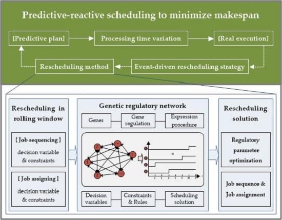
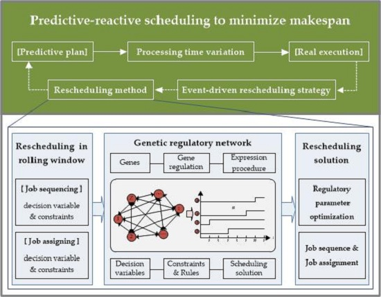
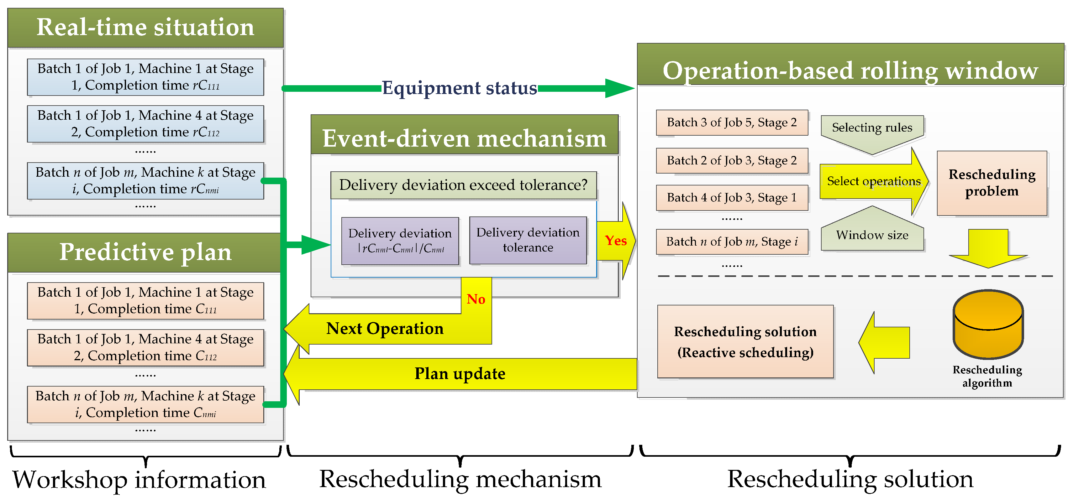
3. Event-Driven Rescheduling Strategy

The predictive-reactive strategy is adopted to realize the dynamic scheduling process in a HFS. According to this strategy, a predictive plan is first developed based on the expected value of processing times. However, there will be a difference between the actual situation and the predictive plan in terms of operation processing times. The event-driven rescheduling mechanism evaluates the disturbance caused by these events and judges the necessity of a reactive scheduling. As shown in Figure 3, taking the objective of minimizing makespan into consideration, the judgment is based on whether delivery time deviation of jobs exceeds a specific tolerance. Delivery time deviation of jobs is calculated as follows:
δ n m = | r C n m I C n m I | / C n m I ,
where CnmI and rCnmI represent expected and actual delivery time of the n th batch of job type m , respectively. If the deviation satisfies δnmI > δmax, a rescheduling is required, otherwise, the predictive plan is kept. A large δmax causes the reactive scheduling insensitive to dynamic events, whereas a small δmax leads to frequent rescheduling. Thereupon, delivery deviation tolerance δmax is an important parameter in the rescheduling strategy.
Moreover, the reactive scheduling is performed within an operation-based rolling window because the processing times are related to operations. As illustrated in Figure 4, the window keeps removing the completed operations and adding the waiting processing ones based on real-time shop information. S(l) represents the set of p operations within the lth window. CS(l) represents the set of completed operations. ES(l) is the set of waiting processing operations. The rolling window forms the rescheduling problem based on S(l) once the reactive scheduling is regarded as necessary. The rescheduling algorithm solves this problem without interrupting the ongoing operations and then generates a new predictive plan based on CS(l) and ES(l), as shown in Figure 3. For each window, a larger p makes the rescheduling problem more complex, but enables better global optimization. On the contrary, a smaller p decreases the computational effort by compromising solution quality. Consequently, the number of operations within each window is also a key parameter in the rescheduling strategy.

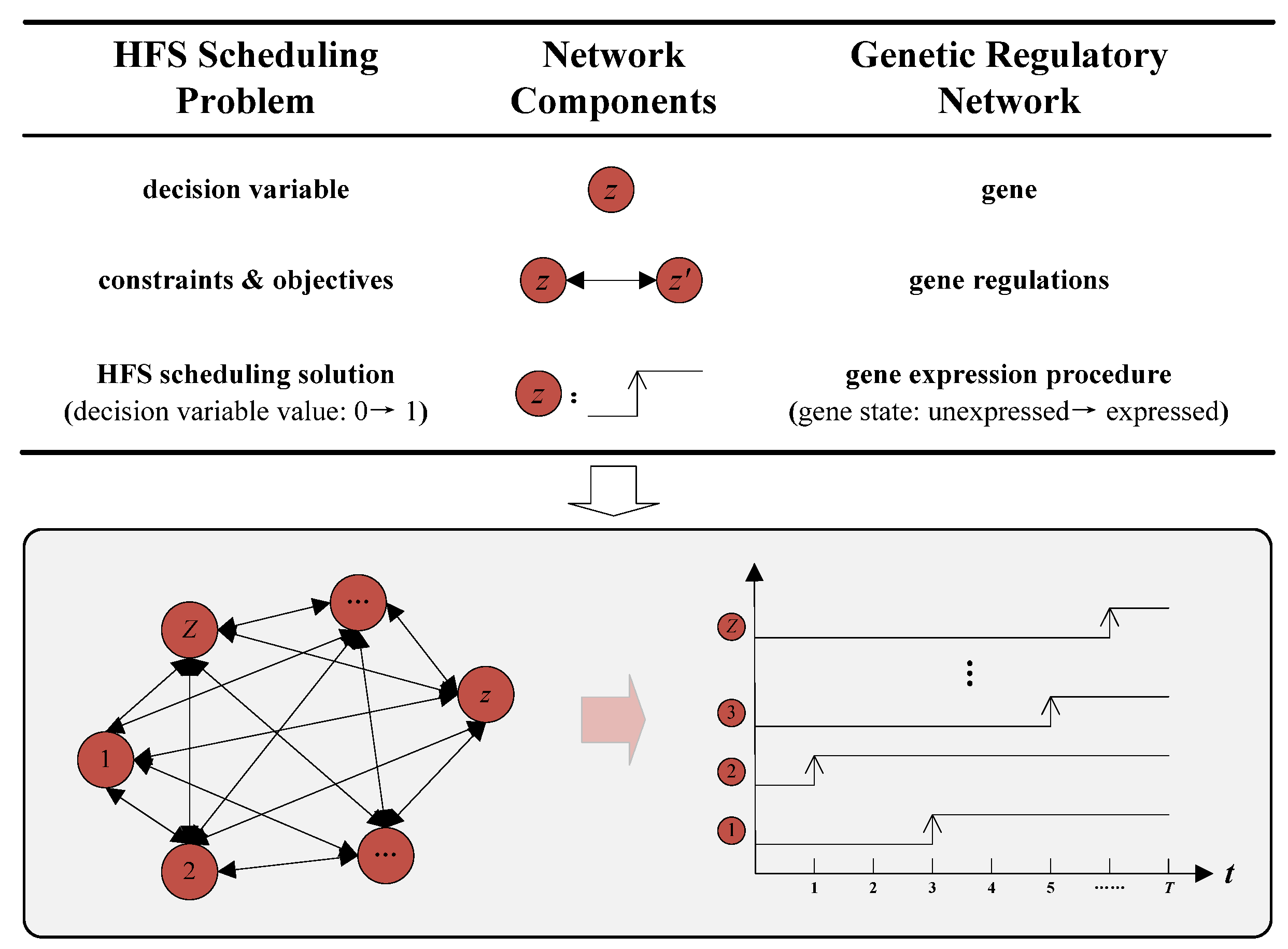
4. Genetic Regulatory Network-Based Rescheduling Method
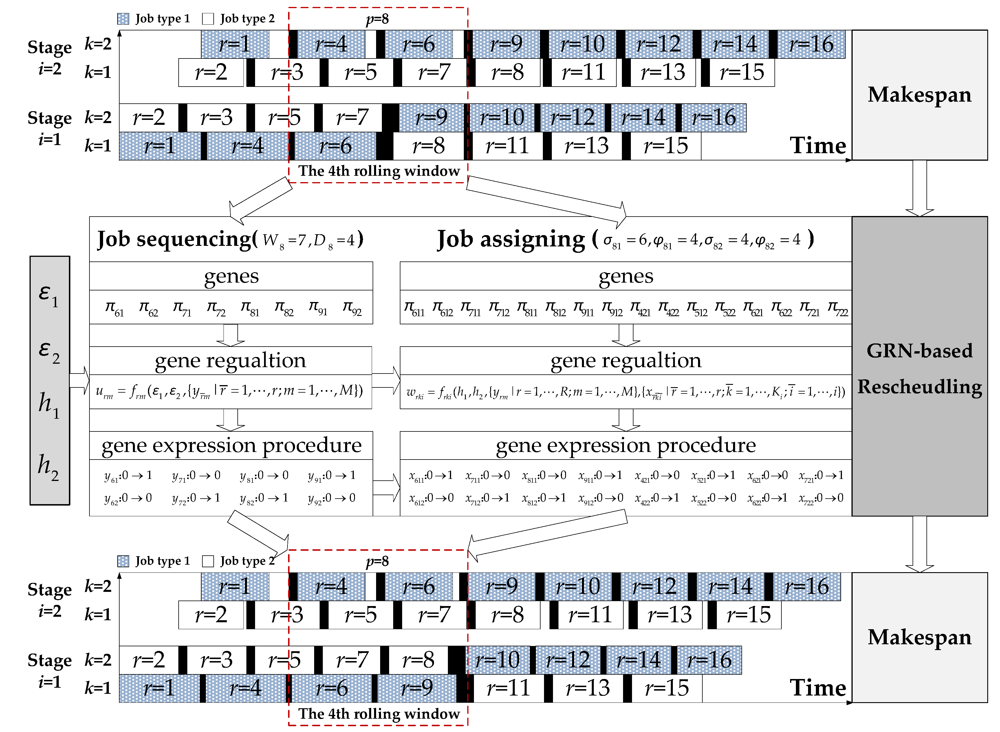
Based on the event-driven mechanism, a rescheduling problem is to be addressed if the delivery time deviation of jobs is larger than the deviation tolerance. A GRN-based method is proposed to solve this problem:
Step (1)
Genes are generated to represent the decision variables. In terms of decision variables yrm and xrki in Table 1, two kinds of genes (i.e., { π r m | r = 1 , 2 , , R ; m = 1 , 2 , , M } and { π r k i | r = 1 , 2 , , R ; k = 1 , 2 , , K i ; i = 1 , 2 , , I } ) are generated. The gene π r m denotes that the r th job entering the HFS belongs to job type m , whereas the gene π r k i denotes that the r th job entering the HFS is processed on the k th machine at the i th production stage.
Step (2)
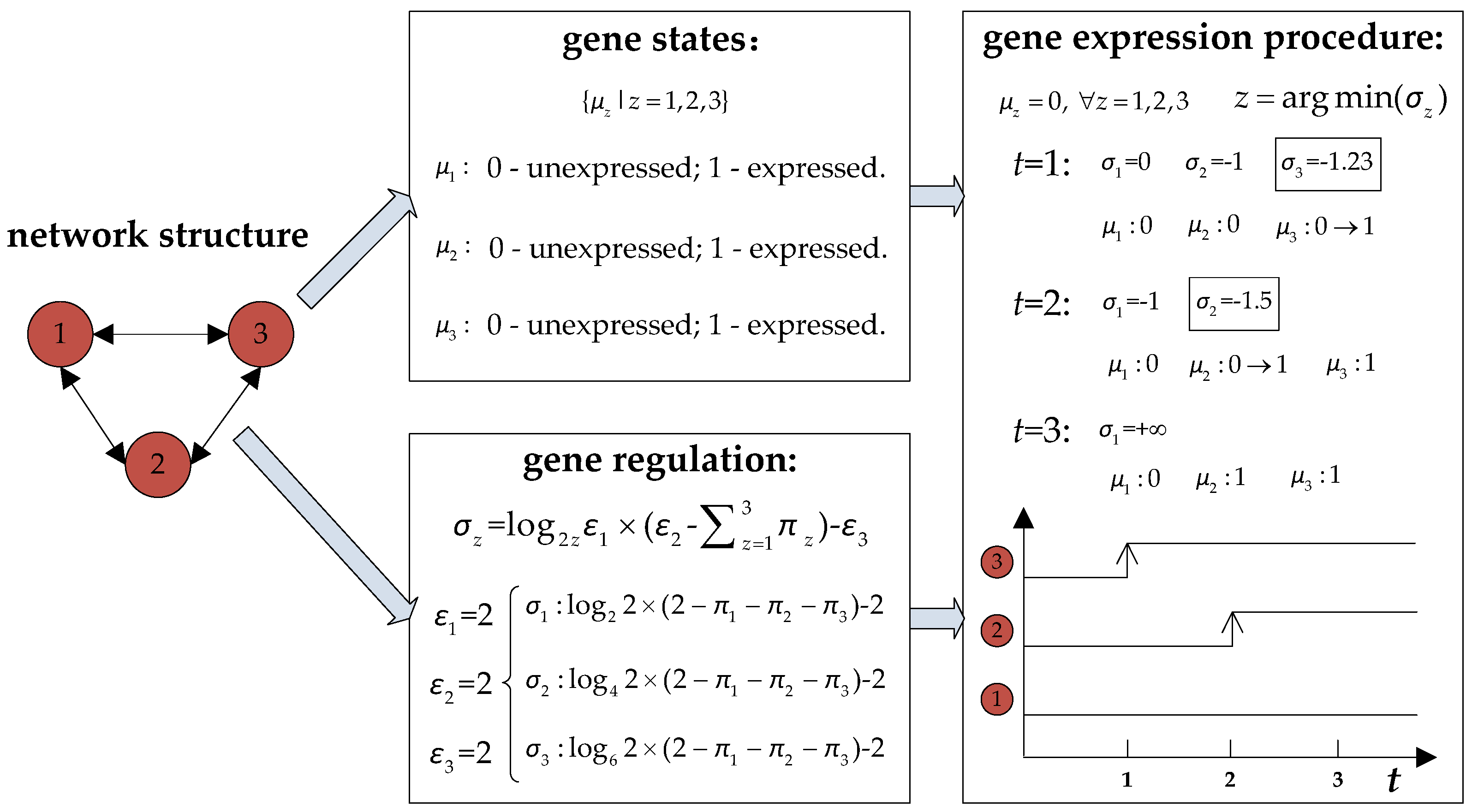
Regulation equations are developed to describe the constraints and objectives:
σ z = f z ( μ 1 ( n ) , μ 2 ( n ) , , μ Z ( n ) , ϑ 1 , ϑ 2 , , ϑ E ) ,
where Z represents the number of genes in a GRN, μ z ( n ) is a binary variable that is equal to 1 if gene π z is in the expressed state at the n th iteration, otherwise, μ z ( n ) is equal to 0, σ z is the inhibition coefficient that describes the inhibitory effects on gene π z quantitatively; ϑ 1 , ϑ 2 , , ϑ E are regulatory parameters; and f z : R ( Z + E ) R is a nonlinear function related to workshop conditions.
Step (3)
Gene expression procedures are designed to determine solutions. At the beginning of such a procedure, the set of related genes is first confirmed based on operations within the rolling window. If a reactive scheduling is necessary, all these genes are initialized to the unexpressed state. At each iteration (i.e., n = 1 , 2 , 3 , , N ), some of these genes are converted to the expressed state based on the regulation equations. When n > N , genes in the expressed state are confirmed, and their corresponding decision variable values are equal to 1 in the rescheduling solution.
Step (4)
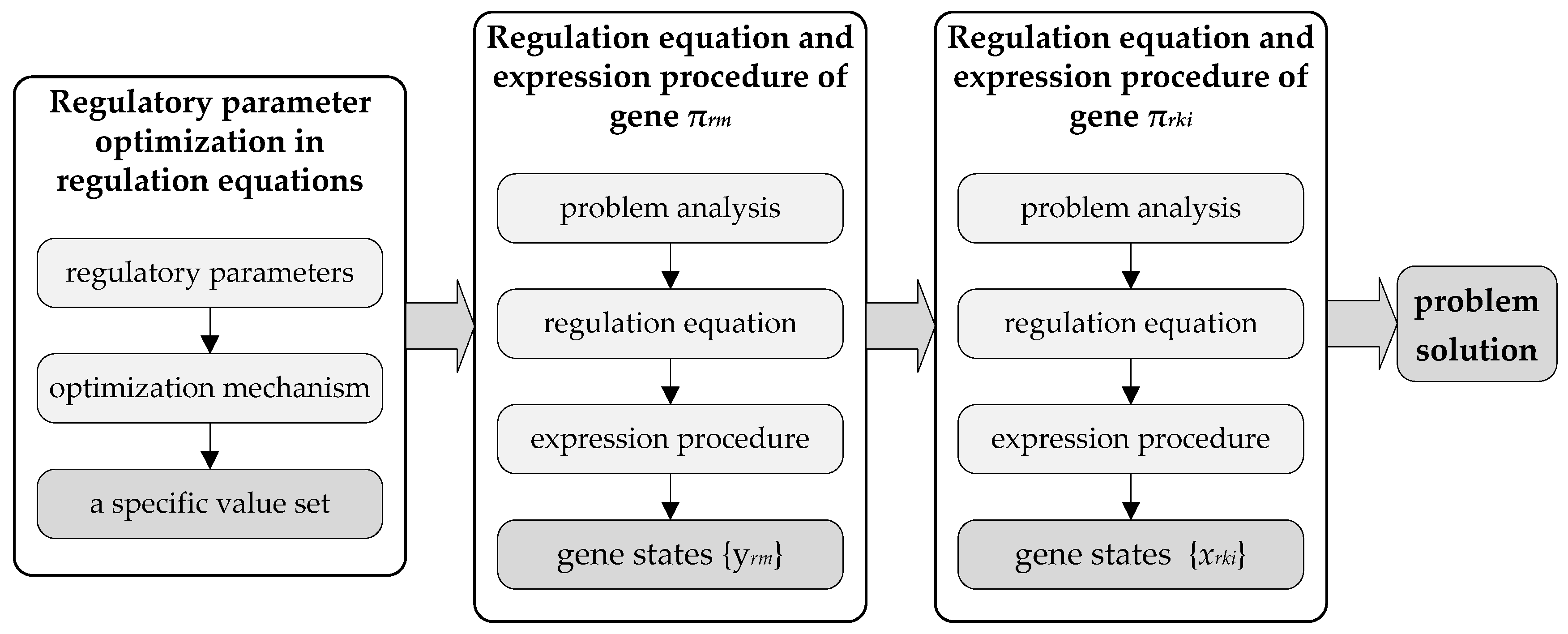
Regulatory parameters are optimized to minimize the makespan. A near-optimal solution is obtained by gene states { y r m | r = 1 , 2 , , R ; m = 1 , 2 , , M } and { x r k i | r = 1 , 2 , , R ; k = 1 , 2 , , K i ; i = 1 , 2 , , I } that are decided by the optimized regulation equations.
As shown in Figure 5, the regulation equation and expression procedure of genes { π r m | r = 1 , 2 , , R ; m = 1 , 2 , , M } and those of genes { π r k i | r = 1 , 2 , , R ; k = 1 , 2 , , K i ; i = 1 , 2 , , I } are presented in Section 4.1 and Section 4.2, respectively. The regulatory parameter optimization procedure is given in Section 4.3.

4.1. Regulation Equation and Expression Procedure of Gene π r m

In HFS scheduling, each machine prefers to operate on the same job type in order to reduce the setup time. For instance, the jobs of type m1 are operated on the 1st machine (i.e., the jobs on this machine are thus “m1-m1-m1-m1-…”), and those of m2 and m3 are assigned to the 2nd machine and the 3rd machine, respectively. In this case, the job sequence entering this production stage will be “m1-m2-m3-m1-m2-m3-…” because the parallel machines perform their tasks simultaneously. Thereupon, each job type would appear in the job sequence cyclically, and the related cycle time should be accorded with the number of parallel machines at each stage. However, the greedy nature of rule-based sequencing methods will probably keep the HFS scheduling choosing the “easy” jobs, which means jobs of a “hard” type will be left to the last positions of the job sequence. For instance, four jobs of type m4 might be left for the last four positions of a job sequence, which is not preferred because there is no scheduling flexibility when assigning these jobs to parallel machines. On the contrary, it is much better to leave four jobs m1, m2, m3 and m4 for remaining positions because the job assigning procedure can choose machines with shorter processing time, less changeovers or earlier availability for each job to minimize the makespan further. For this reason, it is necessary to keep the stable production rate of each job type in the job sequence in order to avoid the near sightedness of rule-based sequencing methods. In terms of these facts, following rules should be obeyed:
  • A job type cannot be selected if its cycle of entering the HFS is not accord with the number of parallel machines at each stage;
  • A job type cannot be selected if its production ratio differs from its demand ratio.
No model sequence could satisfy all these rules completely, and each unsatisfied case might increase the makespan. The regulation equation of gene π r m is thus developed as follows:
u r m = ε 1 i = 1 I | v = 1 r 1 y v m + 1 r   1 K i | + ε 2 | v = 1 r 1 y v m + 1 r   d l m D l | + H ( v = W l r 1 y v m d l m ) + H ( m = 1 M y r m ) ,
where u r m represents the inhibition coefficient to gene π r m , d l m represents the number of job type m entering the HFS within the l th window, D l = m = 1 M d l m , W l represents the number of jobs having entered the HFS before the l th window, ε 1 and ε 2 are regulatory parameters, and H ( x ) is a step function that satisfies H ( x ) = 0 ( x 0 ) and H ( x ) = + ( x > 0 ) . The first two terms of the right side of Equation (4) represent the inhibition strength to gene π r m owing to Rules 1 and 2, respectively. The last two terms ensure the job sequence to satisfy the predetermined quantity of each job type.
In the expression procedure of gene π r m , all the operations are arranged in an ascending sequence in terms of their starting time in the predictive plan. p operations with their starting time later than the rescheduling instant are selected consecutively in the operation sequence. Assuming that dlm represents the number of operations processed on the first production stage for job type m, there are D l = m = 1 M d l m jobs to be arranged for the job sequence within the l th window (from the W l th position to the ( W l + D l ) th position). The genes { π r m | r = W l , W l + 1 , , W l + D l ;   m = 1 , 2 , , M } are thus initialized to the unexpressed state in the rescheduling problem, whereas the gene states { y r m | r = 1 , 2 , , W l ;   m = 1 , 2 , , M } and { y r m | r = W l + D l + 1 , W l + D l + 2 , , R ;   m = 1 , 2 , , M } are given values based on the predictive plan. The gene expression procedure deals with the gene states { y r m | r = W l , W l + 1 , , W l + D l ;   m = 1 , 2 , , M } . At each iteration n = α ( α { 1 , 2 , , D l } ), the inhibition coefficient u r m is calculated for genes { π ( W l + α ) m | m = 1 , 2 , , M } and the gene with minimum u r m is converted to the expressed state. When n > D l , the job sequence within the l th window is rescheduled based on { y r m | r = W l , W l + 1 , , W l + D l ;   m = 1 , 2 , , M } . Appendix A presents this gene expression procedure within the l th window.

4.2. Regulation Equation and Expression Procedure of Gene π r k i

The major objective of assigning jobs to alternative machines is to avoid machine idle time because the makespan is decreased mainly by increasing the utilization of machines. For this reason, the rule of assigning each waiting processing job to the earliest available machine is widely adopted. In addition, each machine prefers to operate on the same job type in order to reduce changeover activities while setup times are taken into consideration. Therefore, assigning a job to parallel machines at each stage should comply with following rules:
  • A machine cannot be selected if the waiting time of a job on this machine is longer than that on another machine.
  • A machine cannot be selected if it requires setup time for a job.
It is almost impossible to satisfy these rules completely, and each unsatisfied case might increase the objective function value. In addition, the 5th assumption should also be obeyed. The regulation equation of gene π r k i is thereby developed as follows:
w r k i = h 1 v = 1 K i ( a r k i a r v i ) + h 2 c b r k i m 0 k i + H ( v = 1 K i x r v i ) ,
where w r k i represents the inhibition coefficient to gene π r k i , a r k i and b r k i represent the end time and the job type of last operation on the k th parallel machine when the r th job enters the i th production stage, m 0 represents the type of the r th job (i.e., m 0 = m = 1 M m y r m ), h 1 and h 2 are regulatory parameters, and H ( x ) is a step function that satisfies H ( x ) = 0    ( x 0 ) and H ( x ) = + ( x > 0 ) . The first two terms of the right side of Equation (5) represent the inhibition strength to gene π r k i owing to Rules 1 and 2, respectively. The last term describes the constraint originated from the 5th assumption. The variable brki satisfies:
b r k i = { b ( r 1 ) k i if x (r1)ki =0 m=1Mmy(r1)mifx(r1)ki =1 ,
and the variable a r k i satisfies:
a rki ={a(r1)kiifx(r1)ki =0 a(r1)ki+cb(r1)kim0 ki+tm0 kiifx(r1)ki =1   and   a r k i k = 1 K i 1 a rk(i1) x rk(i1) k = 1 K i 1 a rk (i1) x rk(i1) + cb(r1)kim0 ki + tm0 ki if x ( r1)ki = 1   and   arki< k=1K i1a rk(i1)x rk(i1) ,
Assuming φ l i jobs (from the σ li th position to the ( σ li + φ l i ) th position in the job sequence) enter the i th production stage based on the p = i=1I φ li operations selected for the l th window, the genes { π ( σ li + β i ) ki | βi =1,2,, φ li ; k= 1, 2 , , Ki ;i=1,2,,I} are initialized to the unexpressed state, whereas other gene states are in accordance with the predictive plan. In the expression procedure of gene π rki , at each iteration n = βi + v=1 i1 φ l v ( i=1,2,,I,   βi { 1,2,, φ li } ), the inhibition coefficient w rki is calculated for genes { π ( σ li + β i)ki |k=1,2,,Ki } and the gene with minimum w rki is converted to the expressed state. When n >p , the production plan within the l th window is rescheduled based on gene states { x ( σ li + β i ) ki | βi =1,2,, φ li ; k=1,2 , , Ki ;i=1,2,,I} . The pseudo codes of this procedure are presented in Appendix B.

4.3. Regulatory Parameter Optimization

Based on values of regulatory parameters ε1 and ε 2 , the gene expression procedure governed by Equation (4) determines the gene states {y rm |r=1,2,,R;  m=1,2,,M} within the l th window, each of which represents whether the r th job entering the HFS belongs to job type m . Moreover, the regulatory parameters h1 and h2 specify the gene regulation in Equation (5) and further determine the gene states {x rki |r=1,2,,R;k=1,2,,Ki ;i=1,2,,I} within the l th window. Each gene state x rki represents whether the r th job is manufactured on the k th machine at the i th production stage. In this way, a solution to the rescheduling problem is obtained based on regulatory parameter values (i.e., ε 1 , ε 2 , h1 and h2 ). Figure 6 illustrates this procedure in the rescheduling of a specific HFS.
A parameter optimization procedure is further implemented to minimize the makespan. According to the regulation equations, a gene receives inhibition if its expression breaks scheduling rules, and the inhibition strength is weighted by related regulatory parameters. These parameters have different values because each rule plays its distinctive role in determining an optimal solution. For example, decreasing setup times is important if machines require comparatively longer durations for job type changeovers, and the parameter h2 should have a large value. The sensitivity analysis on makespan can evaluate the importance weights and thus realize regulatory parameter optimization [42]. Alternatively, machining learning methods can also optimize these parameters if there is enough historical data. For instance, a neural network with workshop conditions can be trained to recommend appropriate parameters.
Apart from these analytical and machine learning methods, random searching algorithms (e.g., genetic algorithms and immune learning algorithms) are also alternative to optimize parameters [43]. For instance, each individual in the genetic algorithm can represent a specific value set of regulatory parameters, and the fitness value of this individual can be evaluated based on related makespan. Through a series of genetic operations (i.e., evaluation, crossover and mutation), the best individual in this algorithm determines the minimum makespan. Moreover, a real-coded algorithm should be used in the parameter optimization procedure because the regulatory parameters are real variables.

5. Numerical Results

5.1. Strategy Parameter Analysis

As discussed in Section 3, delivery deviation tolerance and operation-based window size are important parameters in the event-driven rescheduling strategy. To determine appropriate parameter values, the numeric tests listed in Table 2 are presented.
For these numeric tests, a static scheduling result is first obtained by taking the whole planning horizon as a special rescheduling window and using the GRN-based method. A real-coded genetic algorithm is specifically used in this method to optimize regulatory parameters, in which the population size is 200, the maximum generation is 50, the crossover possibility is 0.8, and the mutation possibility is 0.1. Figure 7 illustrates the Gantt chart of static scheduling results (makespan = 392 s). In this diagram, white rectangles represent processing times and black ones denote changeover times. Moreover, the numbers within each rectangle represents the batch of a job type. For instance, “1, 3” represents the third batch of the first job type.
Assuming that the processing times follow a 4-order Erlang distribution, the rescheduling strategies with different deviation tolerances and window sizes are then used. Table 3 lists the makespan, rescheduling times and computational time of strategies with different deviation tolerances while the window size is 20 operations. In this table, the strategy with the delivery time deviation tolerance of 0.125 minimizes the makespan. Table 4 thus lists dynamic scheduling results with different window sizes while the delivery time deviation tolerance is 0.125. Based on these results, the delivery deviation tolerance of 0.125 and the window size of 77 operations are adopted to generate dynamic scheduling results, as shown in Figure 8.

5.2. Comparative Experiments

Nine benchmarks from Qin et al. [44] are further used to validate the effectiveness of the GRN-based method, as shown in Table 5. Assuming that actual processing times follow the Erlang distribution, these benchmarks are solved by the GRN-based method and the Improved Ant Colony Algorithm (IACO) introduced in [44], respectively. An Intel® CoreTM i7-2720QM CPU @ 2.20 GHz and 8.00 GB RAM based notebook computer (Dell Inc., Xiamen, China) is adopted to test these experiments. Table 6 lists the experimental results. Because both the IACO and the GRN-based method are based on random search procedures, all these results are averaged values over 20 replications.
As shown in Table 6, the IACO method achieves better results than the GRN-based methods for the benchmarks “6 × 2”, “30 × 2” and “100 × 2”. Because these benchmarks are featured with a small-scale solution space, the IACO method is possibly to search out the optimal solutions via its global searching procedure, whereas the GRN-based method might fail to find an optimal one owing to the predetermined rules embedded in its regulation equations. When the problem scale increases in the benchmarks “6 × 4” to “100 × 8”, the GRN-based method obtains smaller makespans than the IACO method. The IACO can hardly search out optimal solutions, or even near-optimal ones, when the solution space is increased, whereas the GRN-based method ensures a good solution owing to its embedded rules and can further find a better one by optimizing regulatory parameters. Moreover, the GRN-based method optimizes four parameters, rather than all the decision variables in the IACO method. This proposed method can thus save the CPU time and demonstrate better response capability to processing time variations in HFS.
Thereupon, the GRN-based method is validated as an effective and efficient method for dynamic scheduling in HFS.

5.3. Case Study

A specific PCB assembly shop composed of four production stages (SMT chip processing stage, plug processing stage, welding processing stage, and test stage) are also investigated. At each production stage, several production lines are alternative for PCB assembly (S1, S2 and S3 at the 1st stage; M1 and M2 at the 2nd stage; A1 and A2 at the 3rd stage; and T1 and T2 at the 4th stage). Ten types of PCBs are assembled in these lines. The requirement for each PCB type is 1000. The processing times and setup times are listed in Table 7 and Table 8, respectively.
Figure 9 illustrates the Gantt chart of static scheduling results obtained by using the GRN-based method. As shown in this figure, all PCB products are divided into 100 batches, and the makespan is 3308 s. Because the starting time of operations is directly determined by the end time of the former operation on the same machine or that of the same job, the processing time variations have cumulative impacts on the completion time of jobs. Based on static scheduling results, the IACO method is used to deal with processing time variations. Figure 10 is the Gantt chart obtained by the IACO method, in which the makespan is 3415.77 s. The GRN-based method is also used to solve the dynamic scheduling problem and achieves a makespan of 3261.98 s, as shown in Figure 11. By integrating job sequencing rules and job assigning rules in a reasonable manner, the GRN-based method ensures waiting jobs to be in-time assigned to an idle machine with comparatively shorter setup time. The regulatory optimization procedure realizes the tradeoff between shorter job waiting time and less changeover activities to minimize the makespan. However, the IACO method fails to realize these targets for some rolling windows because its global search procedure can hardly search out optimal solutions for a real-time scheduling. Taking the first production stage for example, the Garnet chart in Figure 10 realizes higher utilization of Machine 1 and shorter job waiting time on Machine 3 than that in Figure 11. Consequently, the GRN-based method is a more effective scheduling method than the IACO method.

6. Conclusions

This paper solves the HFS scheduling problem with uncertain processing times based on the predictive-reactive strategy. For the rescheduling problems in response to processing time variation events, a novel GRN-based method is developed to minimize the makespan. The critical factor is the employment of GRN to describe the HFS scheduling problem and some scheduling rules. This enables the regulatory parameter optimization procedure to generate near-optimal rescheduling solutions within the reasonable computational time. The effectiveness of this method over the IACO method was demonstrated by a series of benchmark tests and the case study in a PCB assembly shop.
This paper investigates the dynamic event of processing time variations in HFS scheduling, however, the machine breakdowns are also common in real environments. These events will cause the machines to be unavailable for a certain duration known as Mean Time To Repair (MTTR). To deal with these situations, the dynamic scheduling should first generate a predictive plan with minimum makespan based on the assumptions that all the machines are reliable and that the processing times take their expectation values. The job delivery deviation caused by dynamic events of machine breakdowns as well as processing time variations is then monitored during the execution of this plan. If the deviation is beyond a tolerance, the GRN-based method reschedules the production plan within a rolling window to respond to these events. This method will have very complex regulation equations because the unavailability of failed machines needs to be involved in the calculation of job waiting time and machine idle time. Thereupon, the HFS scheduling will be more challenging when the dynamic events of machine breakdowns are taken into account and it will also have better practical values at the same time. Therefore, in our further work, we will develop an enhanced rescheduling method that deals with the dynamic events of machine breakdowns as well as processing time variations by using the GRN. In addition, we will extend this method to multi-objective scheduling that minimizes the due date of jobs, the idle time of machines, the scheduling adjustment cost, etc.

Acknowledgments

The authors would like to acknowledge the financial support of the National Natural Science Foundation of China (No. 51435009; No. 51275307).

Author Contributions

Youlong Lv and Jie Zhang proposed the method and wrote the paper; Wei Qin conceived and designed the experiments; and Youlong Lv and Wei Qin performed the experiments and analyzed the data.

Conflicts of Interest

The authors declare no conflict of interest.

Appendix A

Pseudo codes of expression procedure of gene π r m :
//initialization of genes related to the ( l + 1 ) th window
for α 1 to D l do
  for m 1 to M do
     r = W l + α
     y r m 0     //all genes are in the unexpressed state
  next;
next;
//expression circulation
for α 1 to D l do
   m 0 1 , u 0 +
   r = W l + α     //current iteration
  for m 1 to M do
    calculate u r m in Equation (4)   //inhibition coefficient of current gene
    if u r m < u 0 then
      m 0 m      //update index of the gene with minimum u r m
      u 0 u r m     //update the minimum u r m
    end if;
  next;
   y r m 0 1    //convert the gene with minimum u r m to the expressed state
next.

Appendix B

Pseudo codes of expression procedure of gene π r k i :
//initialization of genes related to the ( l + 1 ) th window
for i 1 to I do
  for r σ l i to σ l i + φ l i do
    for k 1 to K i do
       x r k i 0     //all genes are in the unexpressed state
    next;
  next;
next;
//real-time shop information
for i 1 to I do
  for k 1 to K i do
     r = σ l i
    get a r k i and b r k i
  next;
next;
//expression circulation
for i 1 to I do
  for r σ l i to σ l i + φ l i do
     k 0 1 , w 0 +
    for k 1 to K i do    //current iteration
      calculate w r k i in Equation (4)    //inhibition coefficient of current gene
      if w r k i < w 0 then
         k 0 k     //index of the gene with minimum w r k i
         w 0 w r k i     //the minimum w r k i
      end if;
    next;
     x r k 0 i 1     //convert the gene with minimum w r k i to the expressed state
     r = r + 1
    for k 1 to K i do
      calculate a r k i in Equation (5)  //update shop information
      calculate b r k i in Equation (6)  //update shop information
    next;
  next;
next.

References

  1. Gholami, M.; Zandieh, M.; Alem-Tabriz, A. Scheduling hybrid flow shop with sequence-dependent setup times and machines with random breakdowns. Int. J. Adv. Manuf. Technol. 2009, 42, 189–201. [Google Scholar] [CrossRef]
  2. Chou, F. Der Particle swarm optimization with cocktail decoding method for hybrid flow shop scheduling problems with multiprocessor tasks. Int. J. Prod. Econ. 2013, 141, 137–145. [Google Scholar] [CrossRef]
  3. Yan, H.S.; Jiang, T.H.; Xiong, F.L. A hybrid electromagnetism-like algorithm for a mixed-model assembly line sequencing problem. Int. J. Ind. Eng. Theory Appl. Pract. 2014, 21, 153–167. [Google Scholar]
  4. Arnaout, J.P.; Rabadi, G.; Musa, R. A two-stage Ant Colony Optimization algorithm to minimize the makespan on unrelated parallel machines with sequence-dependent setup times. J. Intell. Manuf. 2010, 21, 693–701. [Google Scholar] [CrossRef]
  5. Lamothe, J.; Marmier, F.; Dupuy, M.; Gaborit, P.; Dupont, L. Scheduling rules to minimize total tardiness in a parallel machine problem with setup and calendar constraints. Comput. Oper. Res. 2012, 39, 1236–1244. [Google Scholar] [CrossRef]
  6. Grabowski, J.; Pempera, J. Sequencing of jobs in some production system. Eur. J. Oper. Res. 2000, 125, 535–550. [Google Scholar] [CrossRef]
  7. Sawik, T.J. Mixed integer programming for scheduling surface mount technology lines. Int. J. Prod. Res. 2001, 39, 3219–3235. [Google Scholar] [CrossRef]
  8. Wong, T.C.; Chan, F.T.S.; Chan, L.Y. A resource-constrained assembly job shop scheduling problem with Lot Streaming technique. Comput. Ind. Eng. 2009, 57, 983–995. [Google Scholar] [CrossRef]
  9. Yalaoui, N.; Ouazene, Y.; Yalaoui, F.; Amodeo, L.; Mahdi, H. Fuzzy-metaheuristic methods to solve a hybrid flow shop scheduling problem with pre-assignment. Int. J. Prod. Res. 2013, 51, 3609–3624. [Google Scholar] [CrossRef]
  10. Salvador, M.S. A solution to a special class of flow shop scheduling problems. In Symposium on the Theory of Scheduling and Its Applications, 1st ed.; Elmaghraby, S.E., Ed.; Springer: Berlin, Germany, 1973; pp. 83–91. [Google Scholar]
  11. Yan, H.S.; Xia, Q.F.; Zhu, M.R.; Liu, X.L.; Guo, Z.M. Integrated Production Planning and Scheduling on Automobile Assembly Lines. IIE Trans. 2003, 35, 711–725. [Google Scholar] [CrossRef]
  12. Sun, Y.; Zhang, C.; Gao, L.; Wang, X. Multi-objective optimization algorithms for flow shop scheduling problem: A review and prospects. Int. J. Adv. Manuf. Technol. 2011, 55, 723–739. [Google Scholar] [CrossRef]
  13. Rossi, A.; Puppato, A.; Lanzetta, M. Heuristics for scheduling a two-stage hybrid flow shop with parallel batching machines: Application at a hospital sterilisation plant. Int. J. Prod. Res. 2013, 51, 2363–2376. [Google Scholar] [CrossRef]
  14. Chan, F.T.S.; Wang, Z. Robust production control policy for a multiple machines and multiple product-types manufacturing system with inventory inaccuracy. Int. J. Prod. Res. 2014, 52, 4803–4819. [Google Scholar] [CrossRef]
  15. Kis, T.; Pesch, E. A review of exact solution methods for the non-preemptive multiprocessor flowshop problem. Eur. J. Oper. Res. 2005, 164, 592–608. [Google Scholar] [CrossRef]
  16. Ruiz, R.; Vázquez-rodríguez, J.A. The hybrid flow shop scheduling problem. Eur. J. Oper. Res. 2010, 205, 1–18. [Google Scholar] [CrossRef]
  17. Pan, Q.K.; Wang, L.; Gao, L. A chaotic harmony search algorithm for the flow shop scheduling problem with limited buffers. Appl. Soft Comput. 2011, 11, 5270–5280. [Google Scholar] [CrossRef]
  18. Wang, H.; Chou, F.; Wu, F. A simulated annealing for hybrid flow shop scheduling with multiprocessor tasks to minimize makespan. Int. J. Adv. Manuf. Technol. 2011, 53, 761–776. [Google Scholar] [CrossRef]
  19. Yang, J. Minimizing total completion time in a two-stage hybrid flow shop with dedicated machines at the first stage. Comput. Oper. Res. 2015, 58, 1–8. [Google Scholar] [CrossRef]
  20. Mirsanei, H.S.; Zandieh, M.; Moayed, M.J.; Khabbazi, M.R. A simulated annealing algorithm approach to hybrid flow shop scheduling with sequence-dependent setup times. J. Intell. Manuf. 2011, 22, 965–978. [Google Scholar] [CrossRef]
  21. Wang, I.L.; Yang, T.; Chang, Y.B. Scheduling two-stage hybrid flow shops with parallel batch, release time, and machine eligibility constraints. J. Intell. Manuf. 2012, 23, 2271–2280. [Google Scholar] [CrossRef]
  22. Wang, S.; Liu, M.; Chu, C. A branch-and-bound algorithm for two-stage no-wait hybrid flow-shop scheduling. Int. J. Prod. Res. 2015, 53, 1143–1167. [Google Scholar] [CrossRef]
  23. Komaki, G.M.; Teymourian, E.; Kayvanfar, V. Minimising makespan in the two-stage assembly hybrid flow shop scheduling problem using artificial immune systems. Int. J. Prod. Res. 2015, 7543, 1–21. [Google Scholar] [CrossRef]
  24. Sun, L.; Yu, S. Scheduling a real-world hybrid flow shop with variable processing times using Lagrangian relaxation. Int. J. Adv. Manuf. Technol. 2015, 78, 1961–1970. [Google Scholar] [CrossRef]
  25. Tang, L.; Liu, W.; Liu, J. A neural network model and algorithm for the hybrid flow shop scheduling problem in a dynamic environment. J. Intell. Manuf. 2005, 16, 361–370. [Google Scholar] [CrossRef]
  26. Chryssolouris, G. Manufacturing Systems: Theory and Practice, 2nd ed.; Springer Science & Business Media: New York, NY, USA, 2006; pp. 465–597. [Google Scholar]
  27. Mehta, S.V.; Uzsoy, R.M. Predictable scheduling of a job shop subject to breakdowns. IEEE Trans. Robot. Autom. 1998, 14, 365–378. [Google Scholar] [CrossRef]
  28. Yao, F.S.; Zhao, M.; Zhang, H. Two-stage hybrid flow shop scheduling with dynamic job arrivals. Comput. Oper. Res. 2012, 39, 1701–1712. [Google Scholar] [CrossRef]
  29. Feng, X.; Zheng, F.; Xu, Y. Robust scheduling of a two-stage hybrid flow shop with uncertain interval processing times. Int. J. Prod. Res. 2016, 54, 3706–3717. [Google Scholar] [CrossRef]
  30. Chryssolouris, G.; Velusamy, S. Dynamic scheduling of manufacturing job shops using genetic algorithms. J. Intell. Manuf. 2001, 12, 281–293. [Google Scholar] [CrossRef]
  31. Gourgand, M.; Grangeon, N.; Norre, S. A review of the static stochastic flow-shop scheduling problem. J. Decis. Syst. 2000, 9, 1–31. [Google Scholar] [CrossRef]
  32. Joo, B.J.; Choi, Y.C.; Xirouchakis, P. Dispatching rule-based algorithms for a dynamic flexible flow shop scheduling problem with time-dependent process defect rate and quality feedback. Procedia CIRP 2013, 7, 163–168. [Google Scholar] [CrossRef]
  33. Wang, K.; Choi, S.H.; Qin, H.; Huang, Y. A cluster-based scheduling model using SPT and SA for dynamic hybrid flow shop problems. Int. J. Adv. Manuf. Technol. 2013, 67, 2243–2258. [Google Scholar] [CrossRef]
  34. Chryssolouris, G.; Dicke, K.; Lee, M. An approach to real-time flexible scheduling. Int. J. Flex. Manuf. Syst. 1994, 6, 235–253. [Google Scholar] [CrossRef]
  35. Rahmani, D.; Ramezanian, R. A stable reactive approach in dynamic flexible flow shop scheduling with unexpected disruptions: A case study. Comput. Ind. Eng. 2016, 98, 360–372. [Google Scholar] [CrossRef]
  36. Michalos, G.; Makris, S.; Mourtzis, D. A web based tool for dynamic job rotation scheduling using multiple criteria. CIRP Ann. Manuf. Technol. 2011, 60, 453–456. [Google Scholar] [CrossRef]
  37. Sahin, F.; Narayanan, A.; Robinson, E.P. Rolling horizon planning in supply chains: Review, implications and directions for future research. Int. J. Prod. Res. 2013, 51, 5413–5436. [Google Scholar] [CrossRef]
  38. Sun, Y.; Feng, G.; Cao, J. Stochastic stability of Markovian switching genetic regulatory networks. Phys. Lett. A 2009, 373, 1646–1652. [Google Scholar] [CrossRef]
  39. Jong, H.D. Modeling and simulation of genetic regulatory systems: A literature review. J. Comput. Biol. 2002, 9, 67–103. [Google Scholar] [CrossRef] [PubMed]
  40. Wang, Y.; Wang, Z.; Liang, J.; Li, Y.; Du, M. Synchronization of stochastic genetic oscillator networks with time delays and Markovian jumping parameters. Neurocomputing 2010, 73, 2532–2539. [Google Scholar] [CrossRef]
  41. Wahde, M.; Hertz, J. Coarse-grained reverse engineering of genetic regulatory networks. Biosystems 2000, 55, 129–136. [Google Scholar] [CrossRef]
  42. Shan, R.; Zhao, Z.S.; Chen, P.F.; Liu, W.J.; Xiao, S.Y.; Hou, Y.H.; Wang, Z. Network modeling and assessment of ecosystem health by a multi-population swarm optimized neural network ensemble. Appl. Sci. 2016, 6, 175. [Google Scholar] [CrossRef]
  43. Quan, G.Z.; Zhang, Z.H.; Zhang, L.; Liu, Q. Numerical Descriptions of Hot Flow Behaviors across β Transus for as-Forged Ti–10V–2Fe–3Al Alloy by LHS-SVR and GA-SVR and Improvement in Forming Simulation Accuracy. Appl. Sci. 2016, 8, 210. [Google Scholar] [CrossRef]
  44. Qin, W.; Zhang, J.; Song, D. An improved ant colony algorithm for dynamic hybrid flow shop scheduling with uncertain processing time. J. Intell. Manuf. 2015. [Google Scholar] [CrossRef]
Figure 1. An example of GRN (Genetic Regulatory Network) composed of three genes.
Applsci 07 00023 g001
Figure 2. Mapping between the HFS (Hybrid Flow Shop) scheduling problem and a GRN.
Applsci 07 00023 g002
Figure 3. Event-driven rescheduling strategy.
Applsci 07 00023 g003
Figure 4. Operation-based rolling window.
Applsci 07 00023 g004
Figure 5. Outline of the GRN-based method.
Applsci 07 00023 g005
Figure 6. An example of GRN-based rescheduling solution (M = 2, I = 2, k1 = 2, k2 = 2, R = 16, d1 = 8, d2 = 8).
Applsci 07 00023 g006
Figure 7. Gantt chart of a static scheduling.
Applsci 07 00023 g007
Figure 8. Gantt chart of a dynamic scheduling.
Applsci 07 00023 g008
Figure 9. Static scheduling Gantt chart.
Applsci 07 00023 g009
Figure 10. IACO (Improved Ant Colony Algorithm) dynamic scheduling Gantt chart.
Applsci 07 00023 g010
Figure 11. GRN-based dynamic scheduling Gantt chart.
Applsci 07 00023 g011
Table 1. Problem’s notations.
NotationsDefinitions
Sets
{ 1 , , m , , M } Set of job types
{ 1 , , i , , I } Set of production stages
{ 1 , , k , , K i } Set of parallel machines at stage i
{ 1 , , r , , R } Set of waiting processing jobs
Parameters
t m k i Operation processing time of job type m on the k th machine at stage i
c m m k i Changeover time required by the k th machine at stage i to operate on job type m after job type m
d m Production volume of job type m , R = m = 1 M d m
Variables
y r m Binary variable: 1, if the r th job entering the first production stage belongs to job type m ; 0, otherwise
x r k i Binary variable: 1, if the r th job entering the first production stage is processed on the k th machine at stage i ; 0, otherwise
a r k i The time instant the k th machine of production stage i to be available for the r th job
b r k i The job type processed by the k th machine of production stage i before a r k i
Table 2. Strategy parameter analysis experiment.
Problem ParameterNumerical Range
Number of production stages (I)4
Number of parallel machines at each stage (Ki)U[2, 4]
Number of job types (M)4
Production volume of each job type (dm)8
Processing time (tmki) (s)U[20, 30]
Changeover time between same job types (cmmki) (s)U[1, 3]
Changeover time between different job types (cmm′ki) (s)U[5, 7.5]
Table 3. Results of delivery time deviation tolerance experiments.
Delivery Time Deviation ToleranceMakespan (s)Rescheduling TimesComputational Time (ms)
0.025408.083965,708
0.05400.551523,842
0.075401.03711,346
0.1407.2057245
0.125394.3423243
0.15394.9323193
0.2395.2211602
0.25395.2211602
0.3439.46016
0.35439.46019
0.4439.46018
0.45439.46021
0.5439.46019
Table 4. Results of rolling window size experiments.
Rolling Window Size (Operation)Makespan (s)Rescheduling TimesComputational Time (ms)
13394.5423216
26397.5534997
39400.7847914
51394.5649305
64398.1937219
77386.78413,006
90390.3326363
102393.3327519
115389.03418,545
128390.54210,400
Table 5. Nine benchmarks for dynamic HFS (Hybrid Flow Shop) scheduling.
BenchmarkNumber of JobsNumber of StagesNumber of Machines at Each StageProcessing Times (s)Setup Times (s) (Same Jobs)Setup Times (s) (Different Jobs)
6 × 262U[1, 5]U[50, 70]U[3, 5]U[12, 24]
30 × 2302U[1, 5]U[50, 70]U[3, 5]U[12, 24]
100 × 21002U[1, 5]U[50, 70]U[3, 5]U[12, 24]
6 × 464U[1, 5]U[50, 70]U[3, 5]U[12, 24]
30 × 4304U[1, 5]U[50, 70]U[3, 5]U[12, 24]
100 × 41004U[1, 5]U[50, 70]U[3, 5]U[12, 24]
6 × 868U[1, 5]U[50, 70]U[3, 5]U[12, 24]
30 × 8308U[1, 5]U[50, 70]U[3, 5]U[12, 24]
100 × 81008U[1, 5]U[50, 70]U[3, 5]U[12, 24]
Table 6. Results of the GRN (Genetic Regulatory Network)-based method and IACO (Improved Ant Colony Algorithm) method.
Benchmark NameGRN-Based MethodIACO Method
Makespan (s)Rescheduling TimesCPU Time (ms)Makespan (s)Rescheduling TimesCPU Time (ms)
6 × 2256.272.313.3252.791.15164.5
30 × 2573.584.2548.6568.451.6580.3
100 × 2886.231.35354.5855.011.98130.5
6 × 41071.561.226.01098.291.85365.2
30 × 42249.042.3567.52314.211.23906.2
100 × 42532.373.15498.42761.851.3533,538.3
6 × 83471.061.351.73536.511.55921.4
30 × 86859.971.997.66978.141.913,641.4
100 × 87396.415.13055.27646.711.8521,9613.3
Table 7. Processing times (s) of different PCB (Printed Circuit Board) types in each production line.
PCB TypeS1S2S3M1M2A1A2T1T2
3ET0321AF4.61511.20.30.240.60.750.60.6
3ET0322AF4.61510.2930.40.30.60.750.60.55
3ET0100CET110.60.061.50.750.750.40.55
3ET0141CET11.42810.40.240.60.30.550.5
3ET0349CET110.60.40.30.750.750.60.6
3ET0630CET1110.060.240.750.60.550.5
3ET0631CET110.60.060.30.60.750.550.4
3ET0741CET14.6150.2930.60.30.750.60.40.4
3ET0374TEK1.4280.9231.20.40.30.60.30.60.55
3ET0435TEK0.9230.9230.8820.61.50.60.40.60.4
Table 8. Setup times (s) between PCBs.
PCB Type3ET0
321AF
3ET0
322AF
3ET0
100CET
3ET0
141CET
3ET0
349CET
3ET0
630CET
3ET0
631CET
3ET0
741CET
3ET0
374TEK
3ET0
435TEK
3ET0321AF1.5612.588.3713.1210.837.288.377.19.519.2
3ET0322AF5.731.329.647.39.5310.575.7710.6712.139.82
3ET0100CET9.817.231.236.3411.2214.6312.211.0912.986.54
3ET0141CET8.938.2711.621.2812.965.978.65.699.958.02
3ET0349CET14.1210.7310.057.791.3214.269.8314.67.079.29
3ET0630CET8.9310.8310.3610.7914.151.5614.9511.810.8810.12
3ET0631CET9.1412.3214.649.999.377.511.7510.3713.435.48
3ET0741CET12.199.8114.228.999.5214.3314.431.2214.0911.83
3ET0374TEK13.177.7514.3410.127.545.858.446.821.385.03
3ET0435TEK6.447.8912.5213.3410.2813.0110.726.147.851.52

