Fourier Series Learning Control for Torque Ripple Minimization in Permanent Magnet Synchronous Motors

Abstract

A new Fourier Series Learning Controller (FSLC) for velocity control on a Permanent Magnet Synchronous Motor (PMSM) is proposed and implemented. An analysis of the error convergence for the FSLC is presented, and the update law for the Fourier series coefficients is specified. The field-oriented control method is used as a basic element to implement three different controllers for a PMSM. The performance of the FSLC is compared with two control methods, a classical PI (Proportional Integral) controller and an artificial neural network controller. The periodic nature of torque ripple in PMSMs is considered as a periodic disturbance, which must be compensated by the controller. With the FSLC implementation, a substantial reduction of the velocity ripple is obtained. Furthermore, a higher speed of learning is achieved with the FSLC in comparison with the artificial neural network.

1. Introduction

The permanent magnet synchronous motors market is growing due to their competitive cost, efficiency and reliability. These motors have common applications in fast dynamic positioning systems and machine tool spindle drives, because they have one of the highest torque-to-losses ratios [1]. However, these motors have an important disadvantage known as “torque ripple”, which is mainly due to the magnetization and the manufacturing of the windings. Torque ripple causes deterioration of the speed and position trajectory, and at high speed applications, torque ripple causes an increase of acoustic noise and additional energy losses [2]. There are methods to control Alternate Current (AC) motors, such as Direct Torque Control (DTC) and Field-Oriented Control (FOC), which have become powerful and popular control schemes for high performance AC drives, but they present undesired large torque and flux ripples [3,4].

A versatile PMSM (permanent magnet synchronous motors) model for torque ripple together with an adaptive control algorithm are an option for torque ripple minimization [5]. Knowledge about torque ripple harmonics is used for the adaptation of the control algorithm; additionally, a current controller is designed to achieve ripple minimization [5]. Moreover, the torque pulsations vary periodically with rotor position, and they are reflected as velocity ripple, particularly at low speeds. Iterative Learning Control (ILC) is intuitively an excellent choice for torque ripple minimization [6]. Using the periodic nature of torque ripple and based on the component’s harmonic distortion in the time domain of the compensation signal, the Fourier series controller coefficients can be adjusted with the aim of reducing the torque ripple in a PMSM, thus allowing for smoother operation [7].

As the Fourier series of a time function characterizes the frequency property of the signal, the Fourier series can be used as a tool for analyzing the convergence of the iterative learning control rules [8]. Further, the Fourier series can be applied in other cases, especially in periodic phenomena. Periodic disturbances affect many physical systems, and periodic reference tracking is required for some applications [9]. Controllers in the frequency domain have several advantages. The main advantage of designing a repetitive controller in the frequency domain is the simplicity in the control algorithm and the real-time implementation [10]. In an invertible generalized flux/current Switched Reluctance Machine (SRM) model based on the Fourier series expansion, the key features are geometry and material property dependency, flexibility in the choice of Fourier terms for the desired level of accuracy and the existence of the inverse flux and torque models [11].

Fourier series representations using trigonometric functions are most commonly used. However, the exponential form of the Fourier series has also been applied, and it has some advantages, such as smaller and clearer mathematical expressions, which makes it easier to extend conclusions that have been developed in the past [12]. Fourier series also can be seen as Neural Networks (NNs) when the series coefficients are strategically modified. These have some differences from traditional NNs. With Fourier Series Neural Networks (FSNN), without prior knowledge of the system model, all of the nonlinearities and uncertainties of the dynamical system are lumped together and iteratively compensated [13].

Other applications of the FSNN have been for servo systems. Some control laws based on a friction model, for servo systems, cannot accomplish an excellent control performance for specific applications with high precision positioning and low velocity tracking. In order to solve this problem, a Fourier series neural network was introduced to approximate a nonlinear, complex and unknown function caused by the frictional phenomenon [14].

An iterative algorithm based on the Fourier series approximation generates the optimal feedforward to force the state trajectory to converge to a stable sliding surface. Using a Fourier series approximation of tracking error, both the magnitudes and phases of the error can be compensated. Therefore, time delay can be easily handled. The iterative learning controller based on the Fourier series compensates for the deterministic uncertainties, and the feedback controller is responsible for stabilizing the system [15,16,17,18].

Without prior knowledge of the system model, the nonlinearities and uncertainties of the dynamical system that are lumped together with no restrictions on their relationship can be compensated online by an Adaptive Fourier Neural Network (AFNN) [19]. There is another nonlinearity that causes extreme difficulty in system modeling. Flexibility is a potential source of uncertainty that can degrade the control performance and even destabilize the system in some cases. To solve this, a Fourier Neural Network (FNN)-based output feedback learning control scheme was proposed. This learning algorithm was carried out in the Fourier space, and it can guarantee the stability of the closed-loop system and the convergence of the tracking error [20].

Nowadays, the Fourier series in control areas have been applied for aerial robots. The use of a frequency-domain iterative learning scheme for periodic quadrocopter flight, parameterizing the non-causal tracking error compensation as Fourier series, was presented by [21]. Uncertainties, such as measurement noise, inaccuracies of the approximate transfer function or model uncertainty, can be accounted for in the learning step size, and the optimal step size for each frequency component can be computed from the statistical properties thereof [21].

There are complex cases where the controllers require help from Fourier series expansions, like the control of autonomous underwater vehicles (AUV). The bottom-following or seabed tracking of AUV, traversing at constant altitudes from the sea bottom, is a big challenge for controllers. However, using the tools of nonlinear output regulation theory combined with Fourier series expansion and pseudo-spectral methods, it is possible to solve the bottom-following problem without requiring knowledge in advance of the seabed profile and using only one single echo sounder to measure the altitude from the seabed [22].

One of the most important contributions of the expansion in Fourier series is helping as a function approximation (FA) when it is difficult to establish an accurate dynamic model. For example, the approach of estimated Fourier coefficients can be used by a nonlinear controller, which simultaneously achieves accurate and ripple-free torque control and minimizes copper losses in brushless motors [23]. In piezoelectrically-actuated systems, this approach can estimate the system dynamics and uncertainties on-line, and no prior knowledge of system dynamics is required [24,25]. An adaptive iterative learning controller can be designed for nonlinear systems with unknown time-varying parameters to realize the non-uniform trajectory tracking perfectly when the time varying parameters are expanded into Fourier series with bounded remainder terms [26].

Moreover, the problem of modeling and tracking control for a high speed ball screw drive, which includes time-varying parametric uncertainties and disturbances, can be solved when a function approximation technique based on Fourier series expansion is applied to estimate the total uncertainties containing inertia uncertainties, stiffness uncertainties and external disturbances [27].

The Fourier series have been complementary tools for conventional controllers, such as Proportional Integral Derivative (PID). However, the Fourier series convergence depends on the conventional controller stability. Furthermore, to obtain the coefficients of the Fourier series, the continuous Fourier transform has been used, which depends on the period of the function, and it is normally unknown.

In this paper, it is demonstrated that Fourier series, with a finite number of terms and the correct update law for the coefficients, can represent the adequate control signal to stabilize a nonlinear system without the help of other controllers. In this way, Fourier series can be used as a control law even though the reference and/or error are not periodic. Besides, it is verified for periodic disturbances, such as torque ripple in PMSMs, that Fourier series can eliminate these disturbances by providing the correct harmonics with a suitable amplitude.

2. Model Description and Problem Formulation

Some causes of torque ripple can be explained from the PMSM mathematical model. In order to understand the periodic nature of torque ripple in PMSMs, this section is used to review the mathematical model and the additional considerations studied by [7].

The relationship between the three currents of a PMSM ${\mathit{i}}_{abcs}$, the mutual and self-inductances ${\mathit{L}}_s$ and the flux linkages ${\mathsf{\Psi }}_{abcs}$ are given by:

$${\mathsf{\Psi }}_{abcs}={\mathit{L}}_s{\mathit{i}}_{abcs}+{\mathsf{\Psi }}_m$$

(1)

In matrix form:

$$\left[\begin{array}{c}\hfill {\mathsf{\Psi }}_{as}\\ \hfill {\mathsf{\Psi }}_{bs}\\ \hfill {\mathsf{\Psi }}_{cs}\end{array}\right]=\left[\begin{array}{ccc}{L}_{asas}& L_{asbs}& L_{ascs}\\ L_{bsas}& L_{bsbs}& L_{bscs}\\ L_{csas}& L_{csbs}& L_{cscs}\end{array}\right]\left[\begin{array}{c}\hfill i_{as}\\ \hfill i_{bs}\\ \hfill i_{cs}\end{array}\right]+\left[\begin{array}{c}\hfill {\mathsf{\Psi }}_{asm}\\ \hfill {\mathsf{\Psi }}_{bsm}\\ \hfill {\mathsf{\Psi }}_{csm}\end{array}\right]$$

(2)

With the flux linkages, the voltages are defined in the stator windings ${\mathit{u}}_{abcs}$ related to the windings resistances ${\mathit{r}}_s$ and the flux linkages:

$${\mathit{u}}_{abcs}={\mathit{r}}_s{\mathit{i}}_{abcs}+\frac{d{\mathsf{\Psi }}_{abcs}}{dt}$$

(3)

where ${\mathit{r}}_s$ is a diagonal matrix with elements $r_s$ and ${\mathit{u}}_{abcs}={[u_{as},u_{bs},u_{cs}]}^T$. Assuming that the stator windings are displaced by $120°$ and that the flux linkages ${\mathsf{\Psi }}_m$ are periodic functions of the electric position ${\mathsf{\theta }}_r$ with magnitude ${\mathsf{\Psi }}_m$ established by the permanent magnet, it is obtained:

$${\mathsf{\Psi }}_m=\left[\begin{array}{c}\hfill {\mathsf{\Psi }}_{asm}\\ \hfill {\mathsf{\Psi }}_{bsm}\\ \hfill {\mathsf{\Psi }}_{csm}\end{array}\right]=\left[\begin{array}{c}\hfill {\mathsf{\Psi }}_m\sin \left({\mathsf{\theta }}_r\right)\\ \hfill {\mathsf{\Psi }}_m\sin ({\mathsf{\theta }}_r-\frac{2}{3}\mathsf{\pi })\\ \hfill {\mathsf{\Psi }}_m\sin ({\mathsf{\theta }}_r+\frac{2}{3}\mathsf{\pi })\end{array}\right]$$

(4)

From Equations (3) and (1), assuming ${\mathit{L}}_s$ is constant:

$${\mathit{u}}_{abcs}={\mathit{r}}_s{\mathit{i}}_{abcs}+{\mathit{L}}_s\frac{d{\mathit{i}}_{abcs}}{dt}+\frac{d{\mathsf{\Psi }}_m}{dt}$$

(5)

Moreover, to find the electromagnetic torque developed $T_e$, the co-energy $W_c$ is defined:

$$W_c=\frac{1}{2}{\mathit{i}}_{abcs}^T{\mathit{L}}_s{\mathit{i}}_{abcs}+{\mathit{i}}_{abcs}^T{\mathsf{\Psi }}_m+W_{PM}$$

(6)

where $W_{PM}$ is the permanent magnet energy. If P are the number of poles of PMSM, the electromagnetic torque developed is:

$$T_e=\frac{P}{2}\frac{\partial W_c}{\partial {\mathsf{\theta }}_r}=\frac{P{\mathsf{\Psi }}_m}{2}\left(i_{as}\cos ({\mathsf{\theta }}_r)+i_{bs}\cos ({\mathsf{\theta }}_r-\frac{2}{3}\mathsf{\pi })+i_{cs}\cos ({\mathsf{\theta }}_r+\frac{2}{3}\mathsf{\pi })\right)$$

(7)

In order to understand torque ripple in PMSM, some assumptions are reconsidered from the previous model (7); for a non-ideal PMSM, the flux linkages are not perfectly sinusoidal, and the electromotive forces ${\mathit{e}}_{abcs}$ are non-cosine functions, although they are periodic functions with a peak value $E_p$:

$${\mathit{e}}_{abcs}=\frac{d{\mathsf{\Psi }}_m}{dt}=E_p{\mathsf{\omega }}_r\left[\begin{array}{c}\hfill f_{as}({\mathsf{\theta }}_r)\\ \hfill f_{bs}({\mathsf{\theta }}_r-\frac{2}{3}\mathsf{\pi })\\ \hfill f_{cs}({\mathsf{\theta }}_r+\frac{2}{3}\mathsf{\pi })\end{array}\right]$$

(8)

where ${\mathsf{\omega }}_r=\frac{d{\mathsf{\theta }}_r}{dt}$ is the angular velocity and $f_{as}\left({\mathsf{\theta }}_r\right)$, $f_{bs}\left({\mathsf{\theta }}_r\right)$ and $f_{cs}\left({\mathsf{\theta }}_r\right)$ are periodic functions with the same shape as $e_{as}$, $e_{bs}$ and $e_{cs}$ with a maximum magnitude $\pm 1$.

Since electromagnetic torque is given by:

$$T_e=[e_{as}{i}_{as}+e_{bs}{i}_{bs}+e_{cs}{i}_{cs}]\frac{1}{{\mathsf{\omega }}_r}$$

(9)

From Equation (8):

$$T_e=E_p[f_{as}({\mathsf{\theta }}_r)i_{as}+f_{bs}({\mathsf{\theta }}_r-\frac{2}{3}\mathsf{\pi })i_{bs}+f_{cs}({\mathsf{\theta }}_r+\frac{2}{3}\mathsf{\pi })i_{cs}]$$

(10)

Then, electromagnetic torque is periodic with ${\mathsf{\theta }}_r$ and is still independent of frequency. However, to produce a constant electromagnetic torque, current waveforms should be calculated.

Moreover, when winding inductances are non-constant, the electromotive forces also are modified. From Equation (1):

$${\mathit{e}}_{abcs}=\frac{d{\mathsf{\Psi }}_{abcs}}{dt}=\frac{d}{dt}[{\mathit{L}}_s{\mathit{i}}_{abcs}+{\mathsf{\Psi }}_m]$$

(11)

$${\mathit{e}}_{abcs}={\mathit{L}}_s\frac{d{\mathit{i}}_{abcs}}{dt}+{\mathit{i}}_{abcs}\frac{d{\mathit{L}}_s}{dt}+\frac{d{\mathsf{\Psi }}_m}{dt}$$

(12)

In Equation (12), it can be seen that torque ripple is produced due to inductance angular variations. The windings inductances can be different in some time instants, and electromagnetic force varies [28].

From macroscopic viewpoint, the torque produced in a PMSM is given by:

$$T_e=\frac{1}{2}{i}^2\frac{dL}{d\mathsf{\theta }}-\frac{1}{2N^2}{\mathsf{\Psi }}_m^2\frac{dR}{d\mathsf{\theta }}+i\frac{d{\mathsf{\Psi }}_m}{d\mathsf{\theta }}$$

(13)

Equation (13) represents the mutual torque that is used to make the motor shaft turn. With this representation of electromagnetic torque, the relation of developed torque and the variations of the angular displacement that can affect resistances and inductances can be seen. These factors among others produce torque ripple in PMSMs. In this examples, it is possible to see the dependence of torque ripple and the angular position ${\mathsf{\theta }}_r$. Furthermore, when PMSM is controlled, the angular position is periodic, as well as torque ripple, which can be seen as a natural periodic disturbance in PMSMs.

3. Learning Controller Design Using Fourier Series

In this section, the Fourier series learning controller is presented for linear and nonlinear systems. An update law for their coefficients, which assures the system stabilization without the help of other controllers, is shown. The harmonics of the error dynamics are used by the controller, and they are obtained from the discrete Fourier transform (DFT). Thus, the error dynamics does not need to be a periodic function.

A function, that represent the dynamics error of the system, is considered to design the learning controller:

$$s\left(t\right)=e\left(t\right)+\dot{e}\left(t\right)$$

(14)

where $e\left(t\right)$ is the error of the system. For this case, $e\left(t\right)={\mathsf{\omega }}_d-\mathsf{\omega }$ is the difference between the desired velocity and the actual velocity of the PMSM. The controller is designed to decrease the function represented by Equation (14).

Each sampling period $T_s$ is taking a sample of $s\left(t\right)$, and data windows with N terms are formed as $[w_0^k,w_1^k,...,w_{N-1}^k]$. The sample $s^k$ in the k-th instant is assigned to $w_{N-1}^k$, and other values are shifted to the left. Namely, $w_{N-1}^k=s^k,w_{N-2}^k=s^{k-1},w_{N-3}^k=s^{k-2},...,w_0^k=s^{k-(N-1)}$. Each data window $w_j^k$ has a sequence of discrete numbers that can be transformed to the frequency domain by the DFT as follows:

$$X_n^k=\sum _{j=0}^{N-1}{w}_j^k{e}^{-i\frac{2\mathsf{\pi }nj}{N}},n=0,1,...,N-1$$

(15)

Note that a data window $w_j^k$ with N real elements is enough to calculate the DFT from Equation (15). Although the elements of the data window are random numbers, the DFT can be calculated. Then, the signal $s\left(t\right)$ does not need to be periodic. Furthermore, using the Euler formula in Equation (15), the real and imaginary parts of $X_n^k$ are:

$$z_n^k=Re\left\{X_n^k\right\}=\sum _{j=0}^{N-1}{w}_j^k\cos \left(\frac{2\mathsf{\pi }nj}{N}\right),n=0,1,...,N-1$$

(16)

$$y_n^k=Im\left\{X_n^k\right\}=-\sum _{j=0}^{N-1}{w}_j^k\sin \left(\frac{2\mathsf{\pi }nj}{N}\right),n=0,1,...,N-1$$

(17)

Then, the coefficients to return from the frequency domain to the time domain in the k-th instant are calculated as follow:

$$p_0^k=\frac{z_0^k}{N},q_0^k=0$$

(18)

$$p_{\frac{N}{2}}^k=\frac{z_{\frac{N}{2}}^k}{N},q_{\frac{N}{2}}^k=0$$

(19)

$$p_n^k=\frac{2z_n^k}{N},n=1,...,\frac{N}{2}-1$$

(20)

$$q_n^k=-\frac{2y_n^k}{N},n=1,...,\frac{N}{2}-1$$

(21)

From the Inverse Discrete Fourier Transform (IDFT), taking the values of Equation (15) and considering N as an even number, the representation in Fourier series for samples in the k-th window $w_j^k$ is:

$$w_j^k=\sum _{n=0}^{N/2}\left(p_n^k\cos \left(\frac{2\mathsf{\pi }nj}{N}\right)+q_n^k\sin \left(\frac{2\mathsf{\pi }nj}{N}\right)\right),j=0,1,...,N-1$$

(22)

Equation (22) means that minimizing the coefficients $p_n^k$ and $q_n^k$, it is possible to decrease $w_j^k$. The controller proposed is a Fourier series with adjustable coefficients, where each coefficient is modified to contribute to the $p_n^k$ and $q_n^k$ decrease in each sample period. Equation (22) is the Fourier series representation of the dynamics error. The new controller uses the coefficients of this representation, but each coefficient is modified by a gain and adding a special function, which can be seen intuitively as an integral part. Finally, in the k-th instant, the controller output is calculated as follows:

$$u\left(k\right)=\sum _{n=0}^{N/2}\left(a_n^k\cos \left(\frac{2\mathsf{\pi }n(N-1)}{N}\right)+b_n^k\sin \left(\frac{2\mathsf{\pi }n(N-1)}{N}\right)\right)$$

(23)

where:

$$a_n^k={\mathsf{\alpha }}_n{p}_n^k+{\widehat{a}}_n^k,n=0,1,...,\frac{N}{2}$$

(24)

$$b_n^k={\mathsf{\alpha }}_n{q}_n^k+{\widehat{b}}_n^k,n=0,1,...,\frac{N}{2}$$

(25)

where ${\mathsf{\alpha }}_n$ is a gain used to obtain a proportion of the harmonics of the error dynamics. The coefficients ${\widehat{a}}_n^k$ and ${\widehat{b}}_n^k$ will be provided by a learning function, and these coefficients are designed to assure that $p_n^k$ and $q_n^k$ decrease. However, the main controller coefficients $a_n^k$ and $b_n^k$ must keep a value different from zero to produce a control signal for the system. Then, coefficients ${\widehat{a}}_n^k$ and ${\widehat{b}}_n^k$ perform the integral part equivalent in a PID controller. In the frequency domain, the integral part must adjust each coefficient of the main controller, until they converge to the correct values. Using the update law proposed by [16], coefficients ${\widehat{a}}_n^k$ and ${\widehat{b}}_n^k$ are calculated as follows:

$${\widehat{a}}_n^k={\mathsf{\gamma }}_n\sum _{j=0}^{k-1}{p}_n^j,n=0,1,...,\frac{N}{2}$$

(26)

$${\widehat{b}}_n^k={\mathsf{\gamma }}_n\sum _{j=0}^{k-1}{q}_n^j,n=0,1,...,\frac{N}{2}$$

(27)

where ${\mathsf{\gamma }}_n$ is a learning gain for each harmonic and should be selected according to some conditions that will be shown in the next section to assure the convergence of $p_n^k$ and $q_n^k$. Note that the convergence of coefficients $p_n^k$ and $q_n^k$ to zero means that the coefficients ${\widehat{a}}_n^k$ and ${\widehat{b}}_n^k$ also converge to some value.

Note that control law (23) was obtained through the IDFT when the harmonics of the $s\left(t\right)$ were modified. However, from IDFT, in each sample period, a data window with N values is obtained. The control output is one value of that window. Due to the arrangement of data window $w_j^k$, the control law in the k-th instant is $j=N-1$, and for this reason, the control law given by (23) is calculated only with $j=N-1$; other values of this window are not necessary.

Before the control method begins, the initial conditions for window $w_j^k$ and gains ${\mathsf{\alpha }}_n$ and ${\mathsf{\gamma }}_n$ are given. When the experiment starts, a sample of $s\left(t\right)$ is taken, and $w_j^k$ is updated. Later, the coefficients $p_n^k$ and $q_n^k$ are calculated through Equations (18), (19), (20) and (21) followed by the coefficients of the controller $a_n^k$ and $b_n^k$ with Equations (24) and (25). Finally, the control law is calculated from Equation (23), and the algorithm is repeated by taking another sample of $s\left(t\right)$. In each cycle of the algorithm, a new data window $w_j^k$ is obtained, and a new DFT is calculated. Then, it is necessary to restart the summations of the DFT. However, the summations of the learning part are not restarted, because the coefficients ${\widehat{a}}_n^k$ and ${\widehat{b}}_n^k$ have the information accumulated during the experiment. In this way, the controller has the information of the error dynamics, and also, it keeps the information of the learning part.

4. Error Convergence Conditions of the Closed-Loop System

The stability of the Fourier series learning controller is shown in this section. The analysis of [16] is extended for this new controller when the Fourier series is the unique controller, and it is not possible to assure that the error dynamics is a periodic function.

First, the change of controller harmonics $\Delta a_n^k$ and $\Delta b_n^k$ is analyzed to find a relation between the controller gains and the change in the harmonics of $s\left(t\right)$. This analysis is important due to the output of a nonlinear system contains, in general, higher harmonics in addition to the fundamental harmonic component [16]. Because the system harmonics are presented in the error signal $s\left(t\right)$, the main objective of controller is to reduce the harmonics of $s\left(t\right)$.

Then, the change of the n-th controller harmonic is represented as:

$$\Delta a_n^k=a_n^{k+1}-a_n^k$$

(28)

where $a_n^{k+1}$ is the next value of the n-th harmonic from the k-th instant. Note that the mathematical procedure in this section is also true for $b_n^k$, $q_n^k$ and ${\widehat{b}}_n^k$.

Additionally, the change in the controller harmonic of $s\left(t\right)$ is calculated as follows:

$$\Delta p_n^k=p_n^{k+1}-p_n^k$$

(29)

where $p_n^{k+1}$ is the next magnitude of the n-th error harmonic from the k-th instant. To determine the stability and conditions for the error convergence of the closed-loop system, the following proposition is described.

Proposition 1.

When the controller (23) is applied to a linear or nonlinear system from which the function (14) can be obtained and the controller coefficients are updated according to Equations (24)–(27), the sufficient conditions for the error convergence are: ${\mathsf{\alpha }}_n>\left|\frac{\Delta a_n^k}{\Delta p_n^k}\right|$ and ${\mathsf{\gamma }}_n<\left|\frac{\Delta a_n^k}{\Delta p_n^k}-{\mathsf{\alpha }}_n\right|$∀$n,k\in {\mathbb{Z}}^{+}$.

Proof. 

The change of controller harmonics is calculated from Equations (24) and (25) as:

$$\Delta a_n^k={\mathsf{\alpha }}_n\Delta p_n^k+\Delta {\widehat{a}}_n^k$$

(30)

where, applying the definition of the change used in Equations (28) and (29), the term $\Delta {\widehat{a}}_n^k$ is:

$$\Delta {\widehat{a}}_n^k={\mathsf{\gamma }}_n{p}_n^k$$

(31)

Substituting Equation (31) into Equation (30), the next expressions can be obtained as:

$$\Delta a_n^k={\mathsf{\alpha }}_n\Delta p_n^k+{\mathsf{\gamma }}_n{p}_n^k$$

(32)

$$\frac{\Delta a_n^k}{\Delta p_n^k}={\mathsf{\alpha }}_n+{\mathsf{\gamma }}_n\frac{p_n^k}{\Delta p_n^k}$$

(33)

$$\frac{\Delta a_n^k}{\Delta p_n^k}={\mathsf{\alpha }}_n+{\mathsf{\gamma }}_n\frac{p_n^k}{p_n^{k+1}-p_n^k}$$

(34)

$$\frac{\Delta a_n^k}{\Delta p_n^k}={\mathsf{\alpha }}_n+{\mathsf{\gamma }}_n\frac{1}{\frac{p_n^{k+1}}{p_n^k}-1}$$

(35)

$$\frac{p_n^{k+1}}{p_n^k}-1=\frac{{\mathsf{\gamma }}_n}{\frac{\Delta a_n^k}{\Delta p_n^k}-{\mathsf{\alpha }}_n}$$

(36)

$$\frac{p_n^{k+1}}{p_n^k}=\frac{{\mathsf{\gamma }}_n}{\frac{\Delta a_n^k}{\Delta p_n^k}-{\mathsf{\alpha }}_n}+1$$

(37)

Taking the right side of Equation (37), the following inequality is possible under certain conditions:

$$-1<\frac{{\mathsf{\gamma }}_n}{\frac{\Delta a_n^k}{\Delta p_n^k}-{\mathsf{\alpha }}_n}+1<1$$

(38)

$$-2<\frac{{\mathsf{\gamma }}_n}{\frac{\Delta a_n^k}{\Delta p_n^k}-{\mathsf{\alpha }}_n}<0$$

(39)

If ${\mathsf{\gamma }}_n>0$, then:

$${\mathsf{\alpha }}_n>\left|\frac{\Delta a_n^k}{\Delta p_n^k}\right|$$

(40)

Furthermore, the other condition that assures the inequality (39) is:

$${\mathsf{\gamma }}_n<\left|\frac{\Delta a_n^k}{\Delta p_n^k}-{\mathsf{\alpha }}_n\right|$$

(41)

With Conditions (40) and (41), the inequality (38) is true, and this means that:

$$-1<\frac{p_n^{k+1}}{p_n^k}<1$$

(42)

In other words:

$$\left|\frac{p_n^{k+1}}{p_n^k}\right|<\mathsf{\beta }<1$$

(43)

where $\{\mathsf{\beta }\in \mathbb{R}|0<\mathsf{\beta }<1\}$. Then, while k increases, in each new sample taken during the experiment, the coefficients $p_n^k$ and $q_d^k$ decrease according to the next sequence:

$$\left|p_n^k\right|<\mathsf{\beta }\left|p_n^{k-1}\right|<{\mathsf{\beta }}^2\left|p_n^{k-2}\right|<\cdots <{\mathsf{\beta }}^k\left|p_n^0\right|$$

(44)

If the coefficients of the Fourier representation of $s\left(t\right)$ are diminished asymptotically, time domain $s\left(t\right)$ is being minimized, namely:

$$s\left(t\right)=e\left(t\right)+\dot{e}\left(t\right)=0$$

(45)

Thus, the above equation represents a stable system, and $e\left(t\right)$ will tend to zero as time increases. ☐

Note that the only conditions for stability are (40) and (41). However, if ${\mathsf{\alpha }}_n$ is chosen so large, the coefficients $a_n^k$ and $b_n^k$ will also be large, but the coefficients $p_n^k$ and $q_n^k$ may or may not be large; it depends of the system and the closed-loop system, which would be unstable if the condition (40) is not satisfied.

The learning gain ${\mathsf{\gamma }}_n$ is upper bounded by condition (41) and lower bounded by zero. However, to make ${\mathsf{\gamma }}_n$ very small means that the learning is very slow and the system control is only ${\mathsf{\alpha }}_n$ dependent. Hence, finding a correct value for ${\mathsf{\alpha }}_n$ can be more difficult.

It is convenient to choose an ${\mathsf{\alpha }}_n$ gain not so large and a ${\mathsf{\gamma }}_n$ not so small. The magnitudes depend only on the system. Furthermore, note that the gains ${\mathsf{\alpha }}_n$ and ${\mathsf{\gamma }}_n$ can be chosen independently for each harmonic. Thus, it is useful to modify the DC components, ${\mathsf{\alpha }}_0$ and ${\mathsf{\gamma }}_0$, independently of the other harmonics. These gains can control a constant energy injected to the system unlike other harmonics, which vary based on the corresponding frequency.

The number of harmonics for the controller depends on the desired response; more harmonics allow an accurate representation of the control signal. However, the number of harmonics is limited by the resonant frequency of the system. Note that a physical system only has a finite bandwidth, and the lower frequency components generally dominate the dynamics error [16]. Furthermore, if a big number of harmonics is chosen, data window $w_j^k$ would have more terms, which requires more memory for the processing system, and it takes more time to calculate the output control.

The sample period is an important factor to be considered. If the sample period is big, the function $s\left(t\right)$ is not correctly represented, and the controller can not assure the stability of the closed-loop system. Note that the DFT can transform any array of numbers, even if they are random numbers, then the Fourier representation of the window $w_j^k$ always exist. Then, the sample period affects only the correct representation of $s\left(t\right)$.

The controller only considers the measurement of the system output compared to the desired output to obtain the output error. Afterward, the function $s\left(t\right)$ and the controller output are calculated. Therefore, the controller does not use the system model, namely the system is decentralized.

5. Experimental Implementation

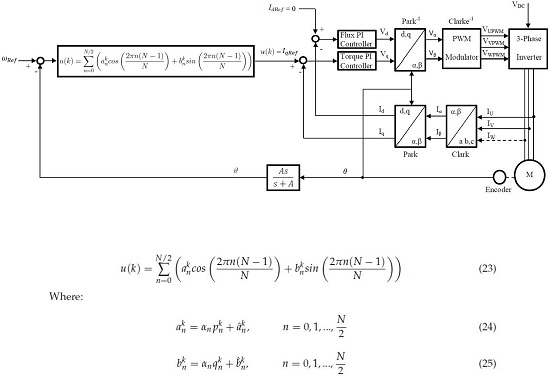
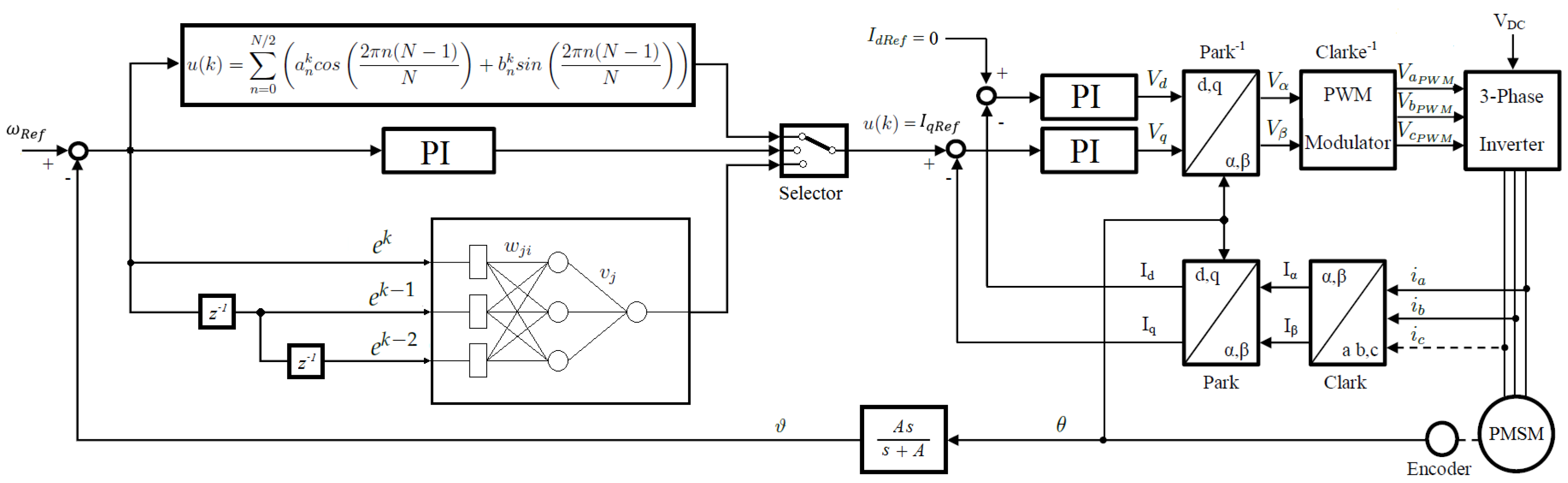
The field-oriented control will be used to implement three different velocity controllers, a Fourier Series Learning Controller (FSLC), a traditional PI controller of the FOC and an Artificial Neural Network (ANN). The performance of the three controllers will be compared. In Figure 1, the block diagram of the FOC for the velocity control of a PMSM with three different master controllers is shown.

The reference value of the flux control $I_{dRef}$ is zero for PMSMs, as is shown in the block diagram [29]. To estimate the angular velocity of PMSM ϑ, a filter of position proposed by [30] is used, which can reduce the noise on the velocity signal compared with the analytical derivative of the angular position. The gain of the filter was $A=5.0$.

The proposed controller is compared with a classical PI control and with an ANN. The architecture and all details of the ANN are those proposed by [31]. We use three neurons in the intermediate layer and three inputs: $e^k$, $e^{k-1}$ and $e^{k-2}$, which are the error and error in two previous instants and one neuron for the output layer.

The controllers will be tested to control the velocity of the EMJ-04APB22 PMSM, which has four poles and the following parameters: 200 (V), $2.7$ (A), 400 (W) maximum power, 3000 (rpm) rated speed, $4.7$ ($\mathsf{\omega }$) stator resistance, $0.014$ (H) stator inductance and 2500 ($PPR$) incremental encoder attached.

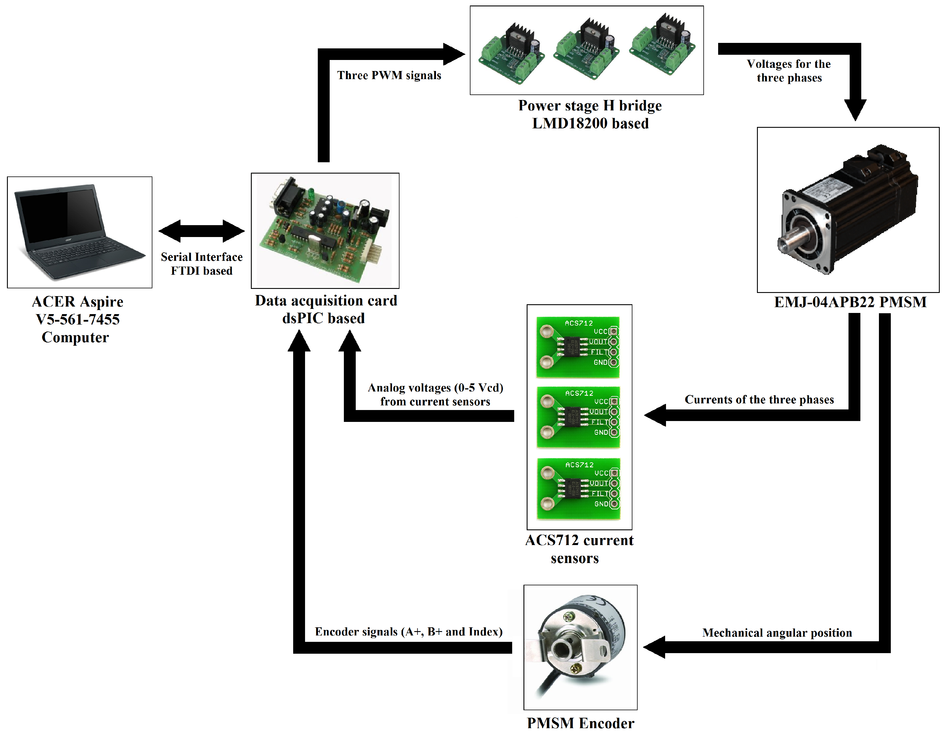
Figure 2 shows the interconnection diagram of the control system. The control algorithms were programed on a computer Aspire V5-561-7455 (acer, New Taipei, Xizhi, Taiwan). The control output values, calculated by the controller, are sent to an acquisition card, which is based on a microcontroller dsPIC33FJ12MC202 (MICROCHIP, Chandler, AZ, USA). For the communication of the microcontroller with the computer, a device FT232RL (FTDI, Seaward Place, Glasgow, UK), was used. The acquisition card has three tasks, to acquire data from the PMSM encoder (Anaheim Automation, Anaheim, CA, USA) and the current sensors, to send data to the computer and to apply three PWM signals to the power stage. The currents of each phase of PMSM are measured from the ACS712 sensors (Allegro, Worcester, MA, USA). The power stage is based on H bridges LMD18200 (Texas Instruments, Dallas, TX, USA), which generate the AC voltages for each phase of the PMSM.

6. Results and Discussion

The reference velocity for controllers and the master PI gains tested in the experimentation, were the lowest velocity and the same gains studied by [32]. In

Table 1. Gains and parameters of the control system.

Description	Parameter	Value
Proportional gain of the slave PI controllers for currents $I_q$ and $I_d$	$K_{ps}$	$1.0$
Integral gain of the slave PI controllers for currents $I_q$ and $I_d$	$K_{is}$	$10.0$
Proportional gain of the FSLC (Fourier Series Learning Controller)	${\mathsf{\alpha }}_n$	$0.037$
Learning gain of the FSLC	${\mathsf{\gamma }}_n$	$0.03$
Number of terms of the FSLC	N	4
Proportional gain of the master PI (Proportional Integral) controller	$K_{pm}$	$0.0477$
Integral gain of the master PI controller	$K_{im}$	$2.38$
Learning coefficient of the ANN (Artificial Neural Network)	$\mathsf{\eta }$	$4.9$
Number of neurons in the intermediate layer of the ANN	$N_n$	3
Gain of the position filter	A	$5.0$
Sample period (s)	$T_s$	$0.005$
Velocity reference (rad/s)	${\mathsf{\omega }}_{Ref}$	$0.3142$

are shown the gains and parameters of the control system. Note that the two slave PI controllers for currents $I_q$ and $I_d$ have the same proportional and integral gains.

The learning coefficient $\mathsf{\eta }$ and the number of neurons in the intermediate layer $N_n$ for the ANN were chosen by observing the dynamics performance of the closed loop system. In the same way, the number of terms N and the gains ${\mathsf{\alpha }}_n$ and ${\mathsf{\gamma }}_n$ of the FSLC were chosen caring the stability conditions (40) and (41) and observing the dynamics performance of the control system. Note that, if ${\mathsf{\gamma }}_n$ is bigger than ${\mathsf{\alpha }}_n$, the stability conditions are not satisfied, and the stability cannot be assured; which is an example of the wrong selection of gains.

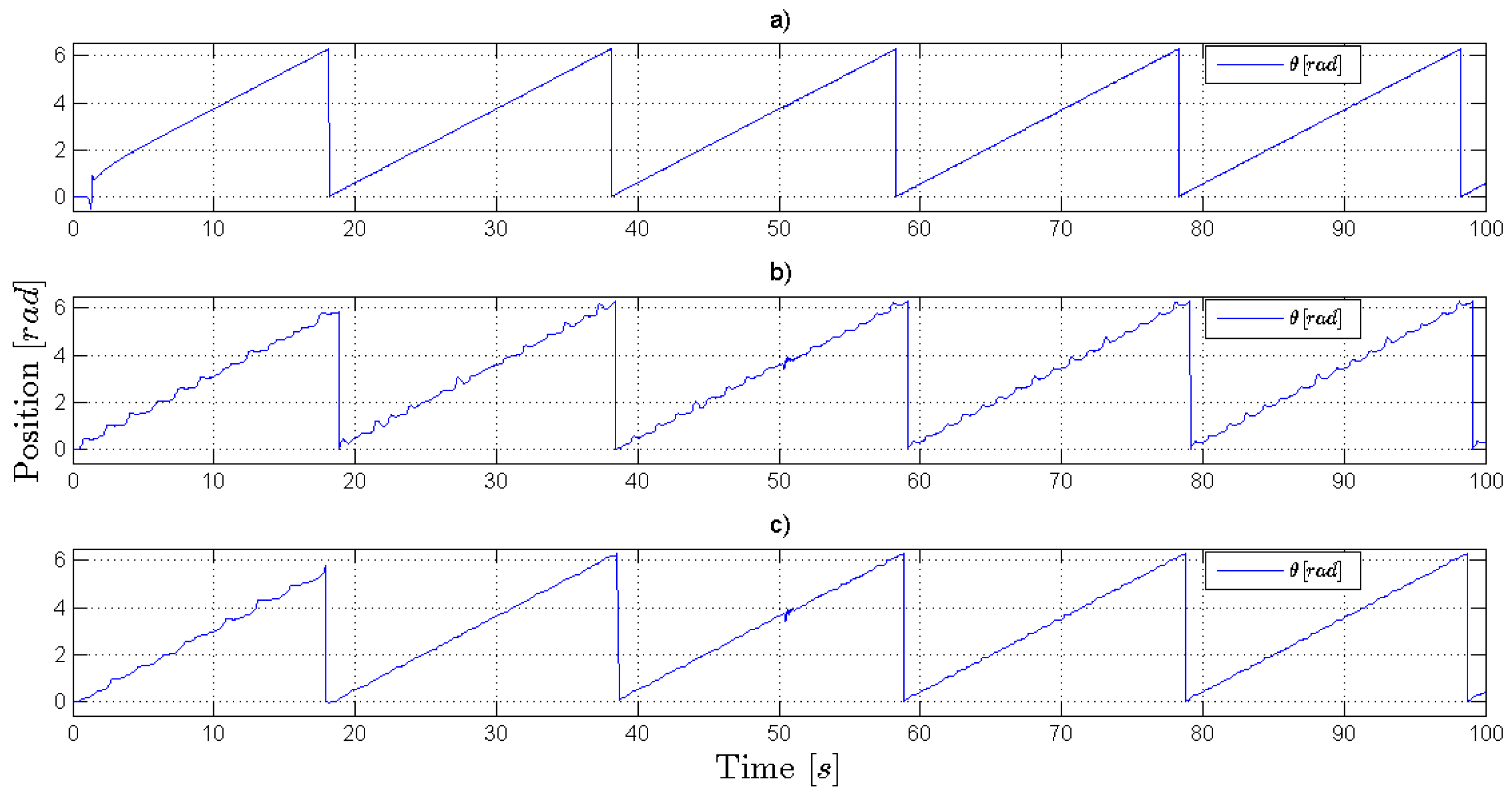
First, the angular position $\mathsf{\theta }$ of the PMSM is shown in order to observe the different performances of the three controllers. A constant velocity must produce a straight line of the angular position from zero to $2\mathsf{\pi }$. Figure 3 shows the behavior of controllers when the velocity of PMSM is controlled. The PI controller cannot reduce the torque ripple, as can be observed in Figure 3b, where a distortion of angular position produced by the torque ripple is shown. The ANN reduces the torque ripple after a learning time of $18.0$ s approximately, as is shown in Figure 3c. However, the Fourier series learning controller reduce the torque ripple faster than the ANN in $2.7$ s approximately, as is shown in Figure 3a. Additionally, a change of load is applied after 50 s. A mass of $1.2$ kg is loaded by the PMSM. According to the rotor size of the motor, the torque generated by this mass is $0.0824$ Nm. It is observed that the three controllers can compensate the constant disturbance; however, the torque ripple continues affecting the PI as the velocity controller.

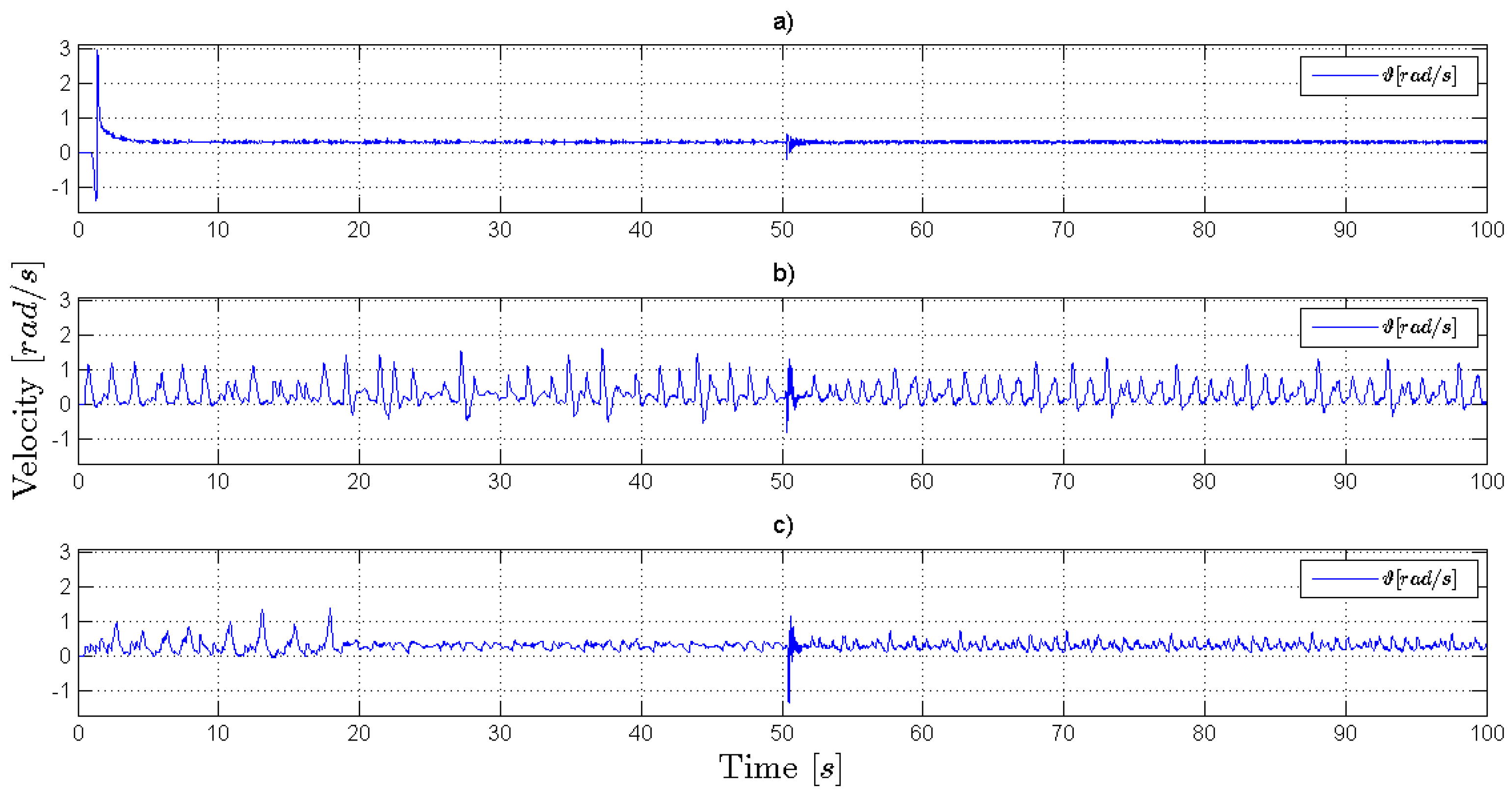
Figure 4 shows the estimation of the velocities ϑ of the closed-loop systems for the three controllers. In Figure 4b is shown the estimation of velocity of the closed-loop system with a PI as the velocity controller. It can be observed that the torque ripple affects the velocity, and the PI cannot compensate it. In Figure 4c is shown the estimation of velocity of the closed-loop system with the ANN as the velocity controller. It can be observed that the speed varies around the desired velocity while the ANN learns, but only after $18.0$ s, approximately, the torque ripple is reduced. In Figure 4a is shown the estimation of velocity of the closed-loop system with the FSLC as the velocity controller. In the first $2.7$ s, during the learning process, a peak of velocity occurs, which is compensated in $0.16$ s, approximately, and later, the velocity ripple is reduced. When the disturbance is applied from 50 s, the three controllers can compensate it, in $1.14$ s, approximately. After the disturbance, the FSLC and the PI controllers are not affected. However, in Figure 4c, it is observed that the ANN is affected before 50 s; namely, the variations of the velocity are bigger than the variations before the disturbance.

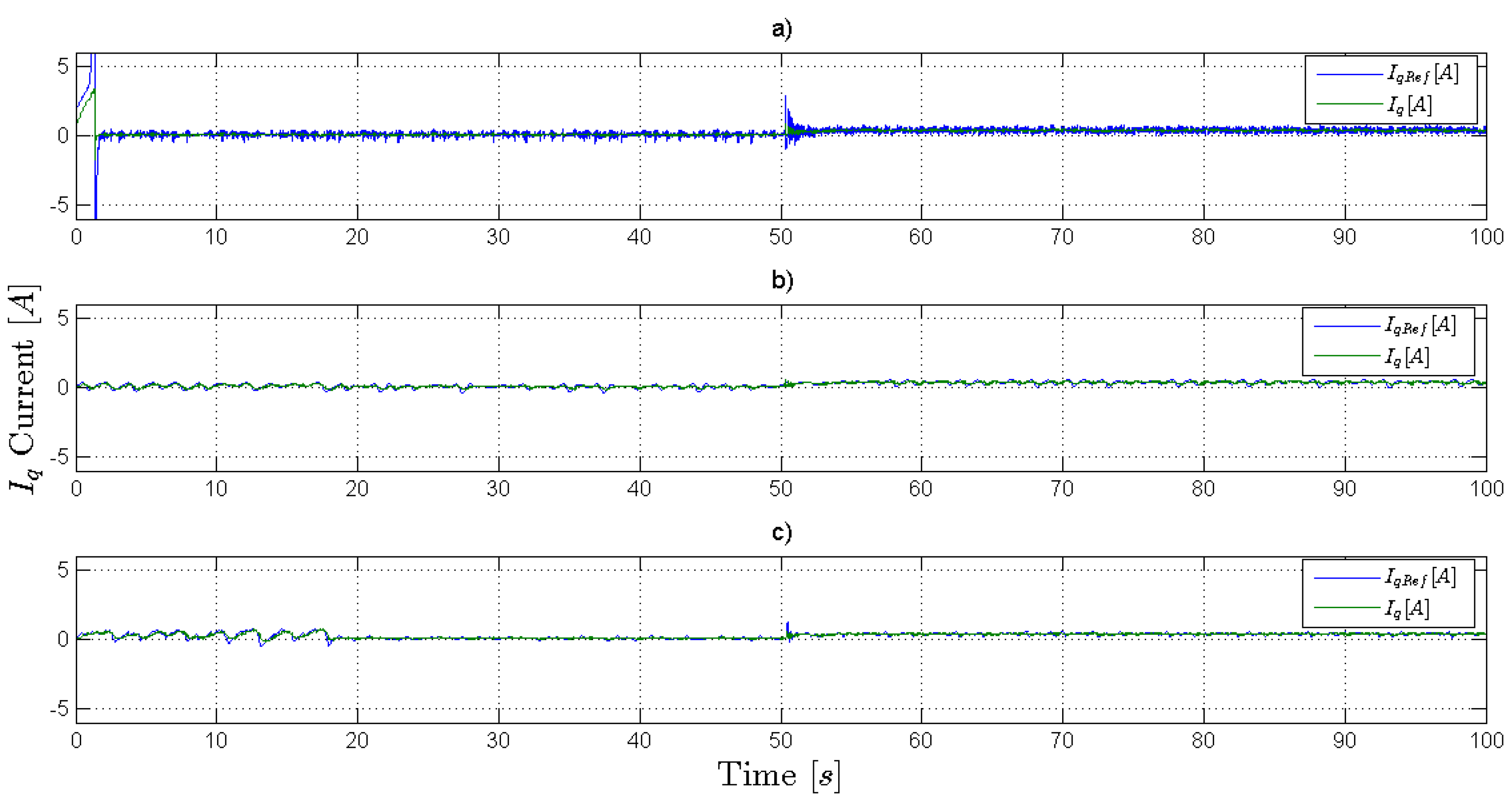
Figure 5 shows the control signals $I_{qRef}$ of controllers and the measured currents $I_q$ of the closed-loop systems. Figure 5b Shows the behavior of the PI controller. It can be observed that the control signal and the current measured $I_q$ are apparently similar, and there are some small variations. Figure 5c shows the behavior of the ANN controller. In the learning stage, there are large variations of the control signal and also of the measured current. After the learning stage, the variations are reduced, and the control signal is similar to the measured current, which corresponds to the moment of the reduction of the velocity ripple. Figure 5a shows the behavior of the Fourier series learning controller. In the learning stage, the control signal increases to $5.5$ A, and it is saturated; however, the measured current only reaches $3.5$ A. Later, the signal control decreases to $-5.5$ A, but the measured current only decrease to $-1.7$ A. After the learning stage finishes, the measured current $I_q$ tries to follow the control signal $I_{qRef}$, and the velocity ripple is reduced. Later, when the torque disturbance is applied from 50 s, the currents are incremented up to $0.5$ A in order for the change of load to be compensated.

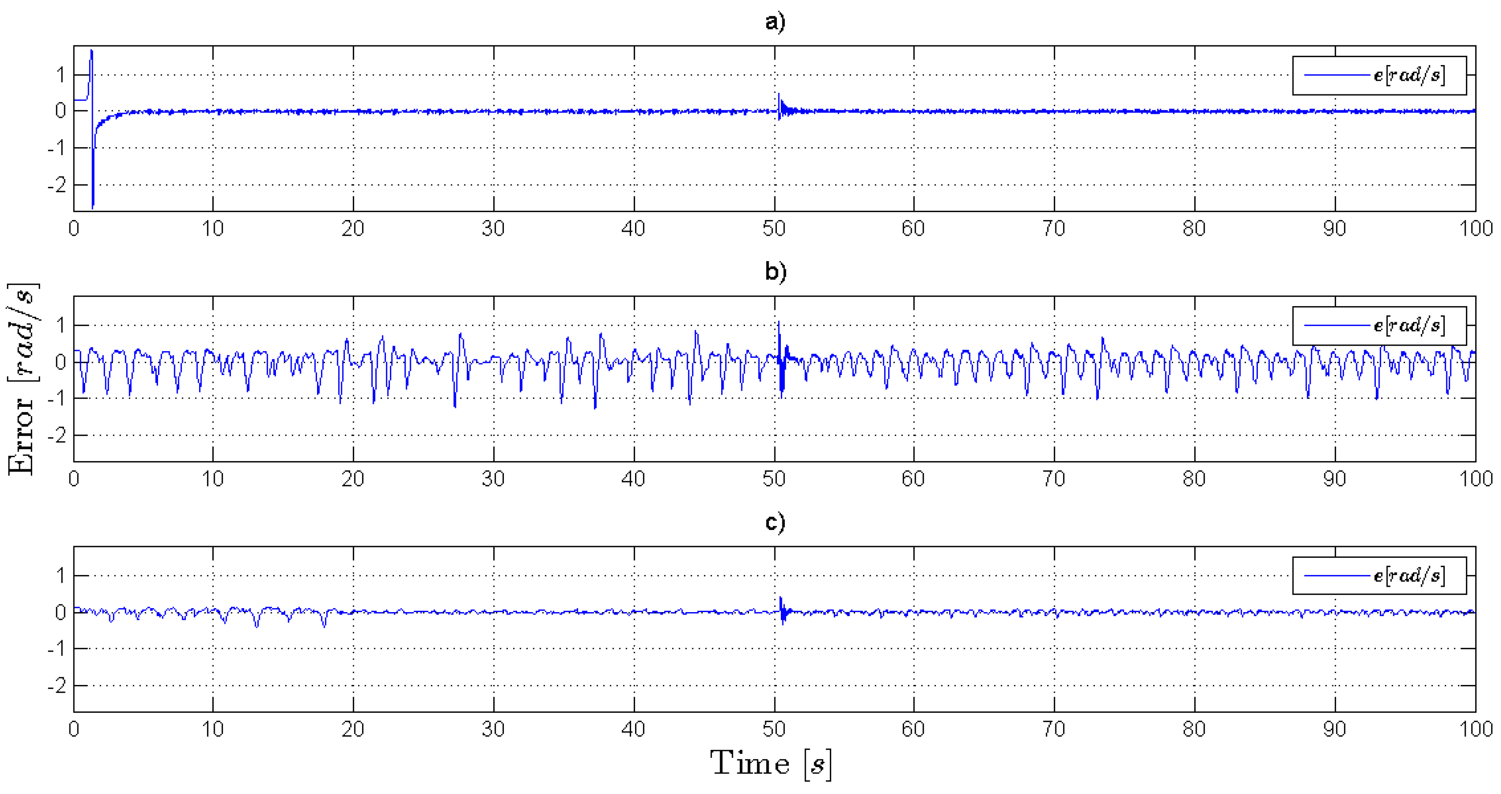
Figure 6 shows the errors of the control systems obtained by each controller. In Figure 6b, it is observed that the PI controller cannot compensate the torque ripple, and the error varies to $-1.2$ rad/s. Figure 6c shows the error obtained when the ANN is the velocity controller. During the first $18.0$ s, there are variations of the error up to $-0.4$ rad/s, but after the learning time, the error oscillates around 0 rad/s, between $-0.07$ and $0.8$ rad/s. In Figure 6a, the error obtained with the FSLC as the velocity controller is shown. During the learning time, the error reaches $-2.5$ rad/s; however, after this time, the error converges, and it remains near zero. Thus, it is experimentally demonstrated that the FSLC achieves the error convergence of a nonlinear system. When the controllers are under a constant disturbance of torque after 50 s, it is shown that this disturbance only affects the ANN as the controller, since from the disturbance, the error varies up to $-0.2$ rad/s. However, in the case of the FSLC as the controller the error continues around zero, and the variations are maintained between $-0.05$ and $0.05$ rad/s. Then, it is experimentally demonstrated that the FSLC can add the integral part in a control system.

7. Conclusions

A new Fourier series learning controller was proposed and applied in a nonlinear system. The error convergence of the Fourier series learning controller was analyzed, and two convergence conditions were obtained. The new controller was used for the velocity control on a PMSM, which reduces the torque ripple by $70\%$ with respect to the results obtained with a PI as the velocity controller.

The performance of the Fourier series learning controller was compared with the performance of other two controllers, the conventional PI controller and an artificial neural network. There were two comparisons against a controller that cannot compensate the torque ripple, and another that can reduce this periodic disturbance. However, it is a valuable study to compare the performance of the FSLC with other techniques for reducing the torque ripple, and this is proposed for future work. In this case, a learning time of 2.7 seconds was required for the FSLC, whereas for the ANN, 18.0 seconds were required. The computational cost of the new FSLC is bigger than the conventional PI controller, since the FSLC requires more code lines and programming loops than the PI. However, the PI controller cannot reduce the torque ripple as the FSLC or the ANN. Nevertheless, the computational cost of the FSLC is considerably less than the ANN, and the results show that the FSLC can learn faster than the ANN. Besides, for the FSLC, the processing time and the computational cost could be reduced if other mathematical tools are applied instead of the DFT as the FFT, which is a good proposal for future work.

The results show that the FSLC is a good alternative to be applied as the controller in the control of nonlinear systems, including the compensation of periodic disturbances, such as torque ripple in PMSMs. The FSLC designed is a model-free controller, and it only requires information of the error dynamics.