
Chronic Inflammation in the Epidermis: A Mathematical Model

Abstract
:
1. Introduction
2. Materials and Methods
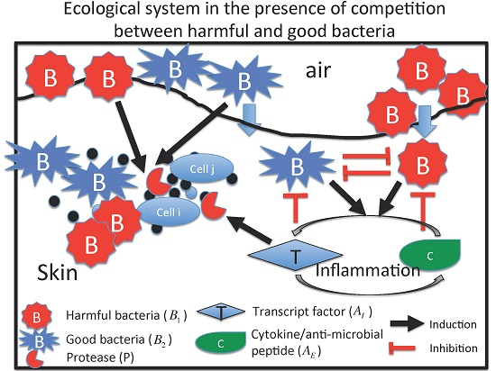
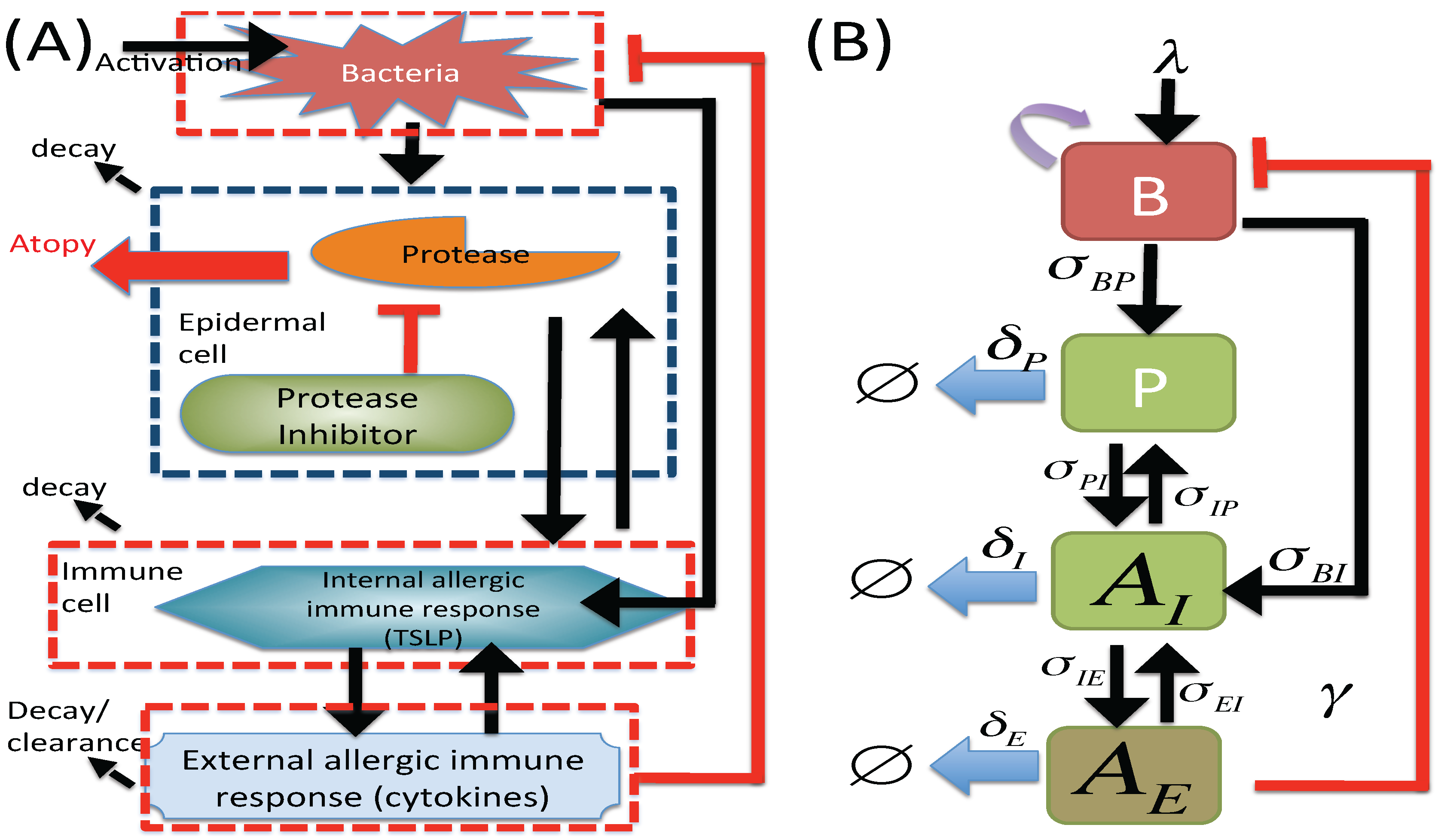
2.1. M1 Model
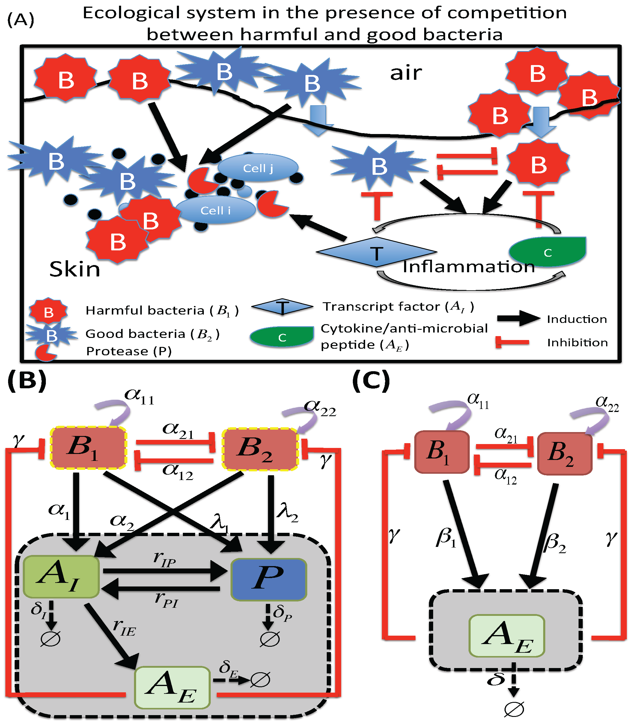
2.2. M2 Model
3. Results
3.1. Dynamics of the M1 Model
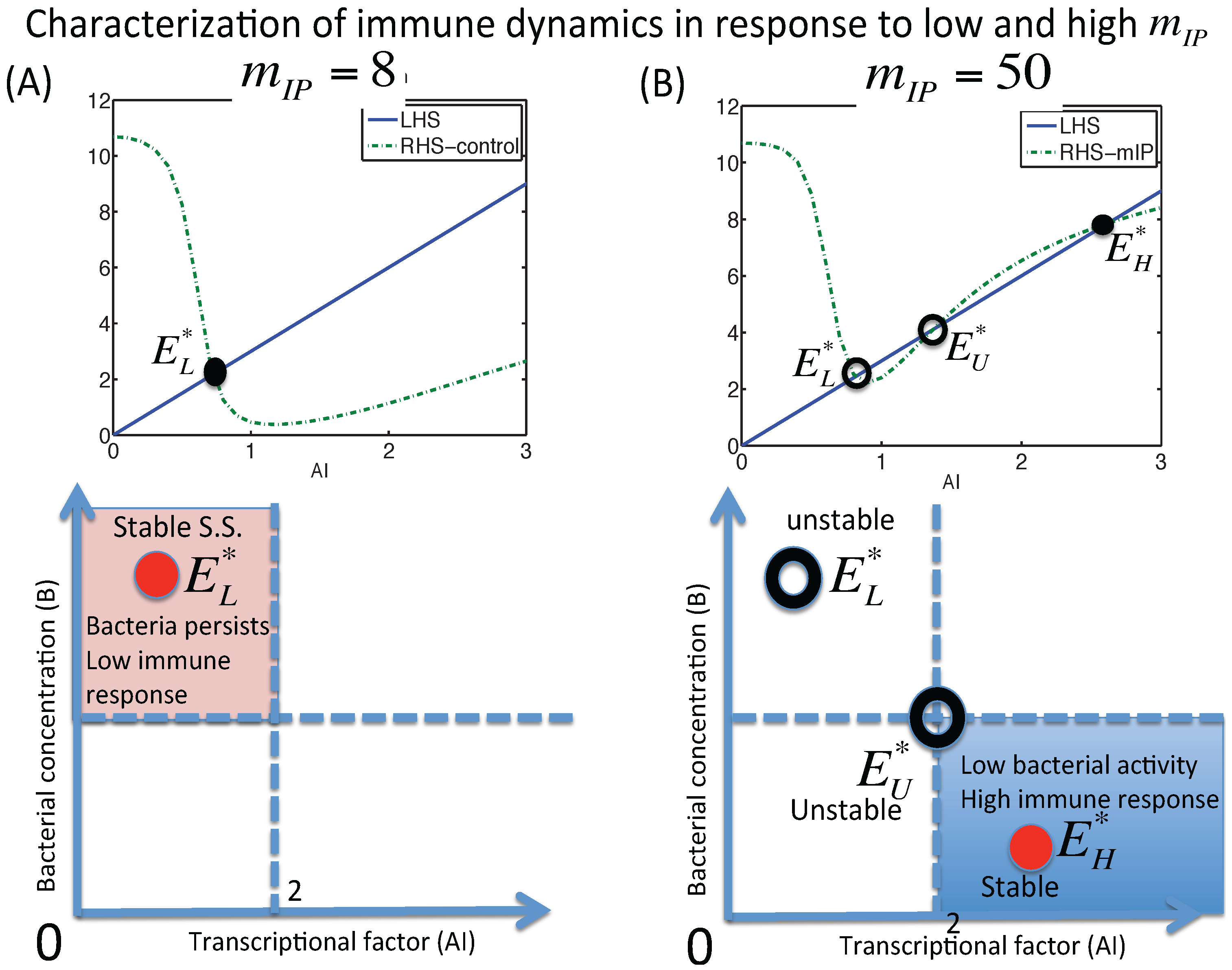
3.1.1. Classification of Steady States
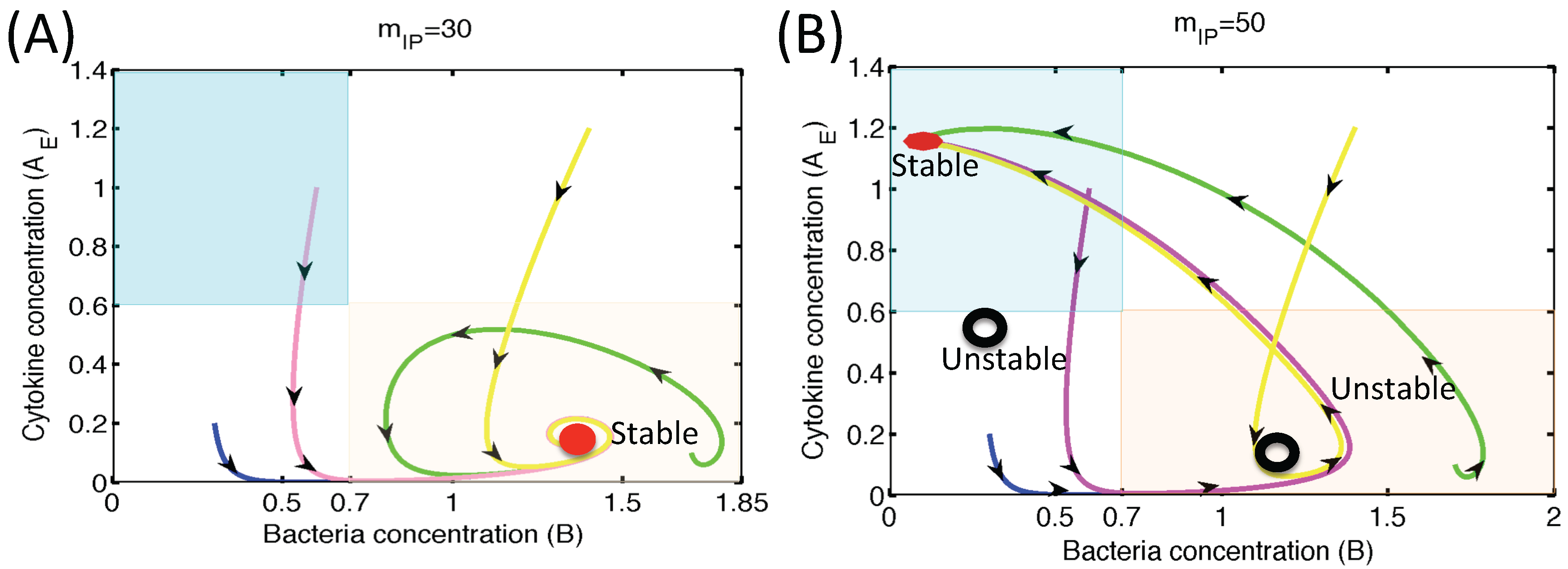
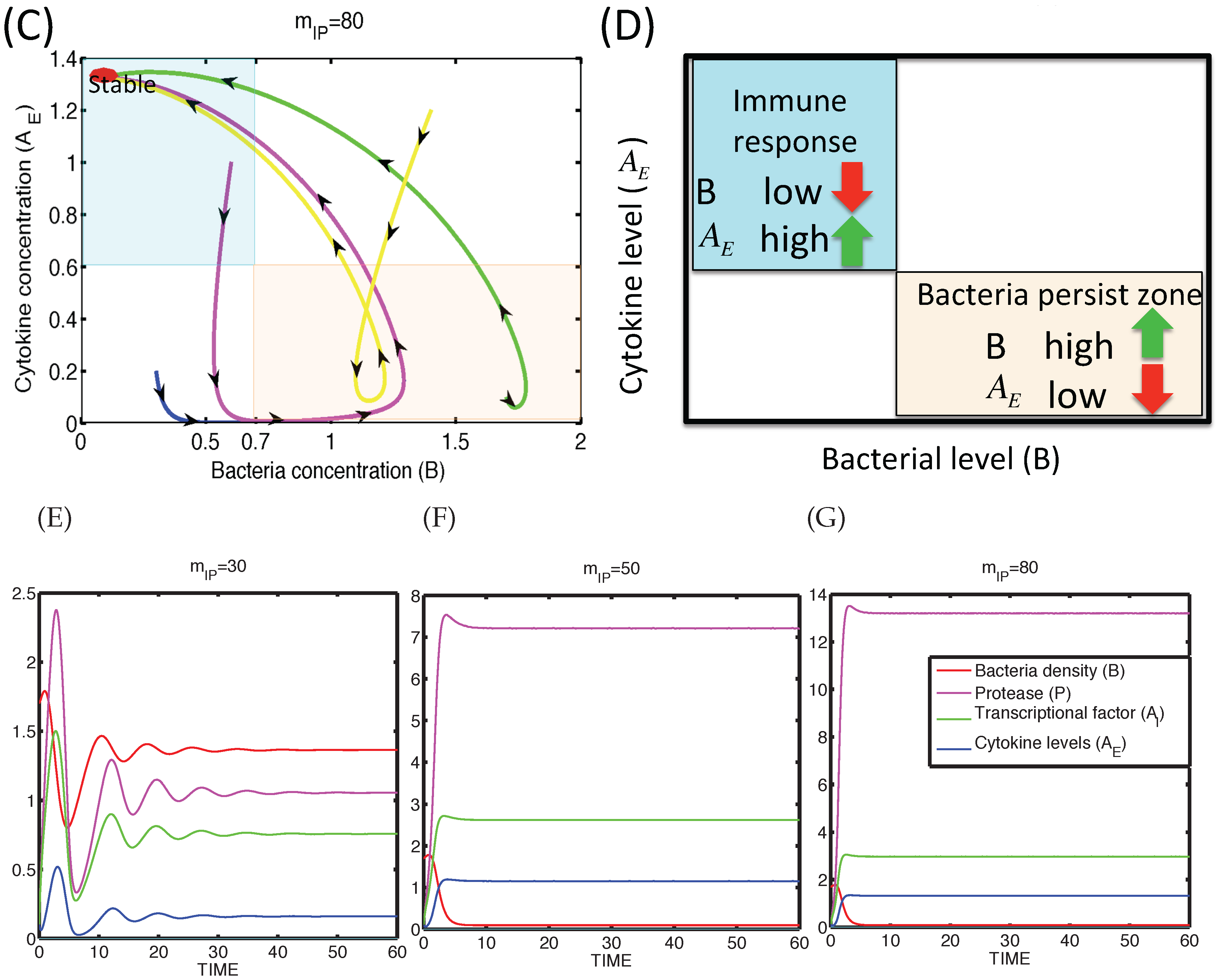
3.1.2. Dynamics of the M1 Model System
3.2. Dynamics of Two Bacterial Strains Model (M2 Model)
3.2.1. Existence of Equilibria
3.2.2. Stability of Equilibria
- (E1S1) and ,
- (E1S2) , and .
- (E2S1) and ,
- (E2S2) , and .
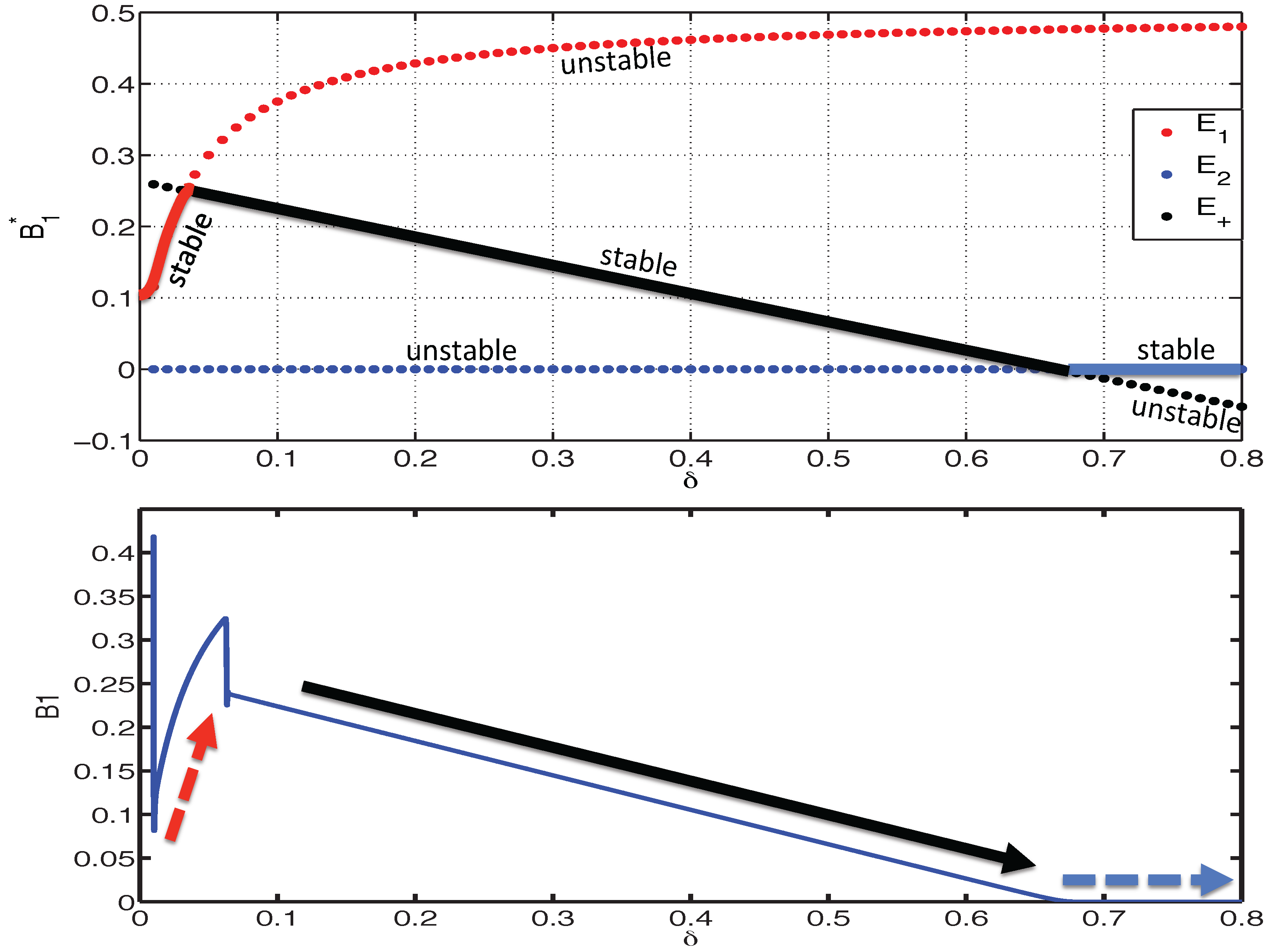
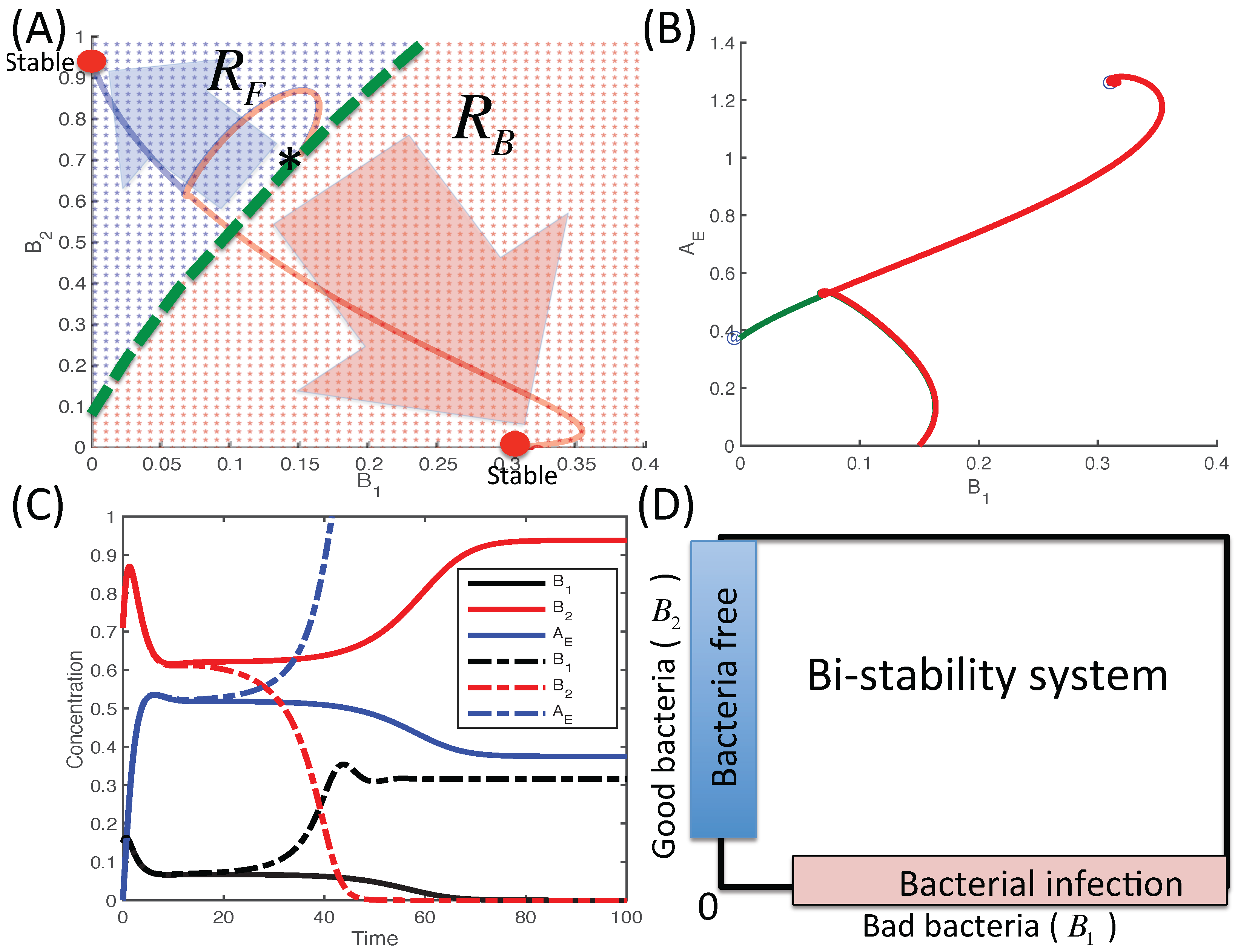
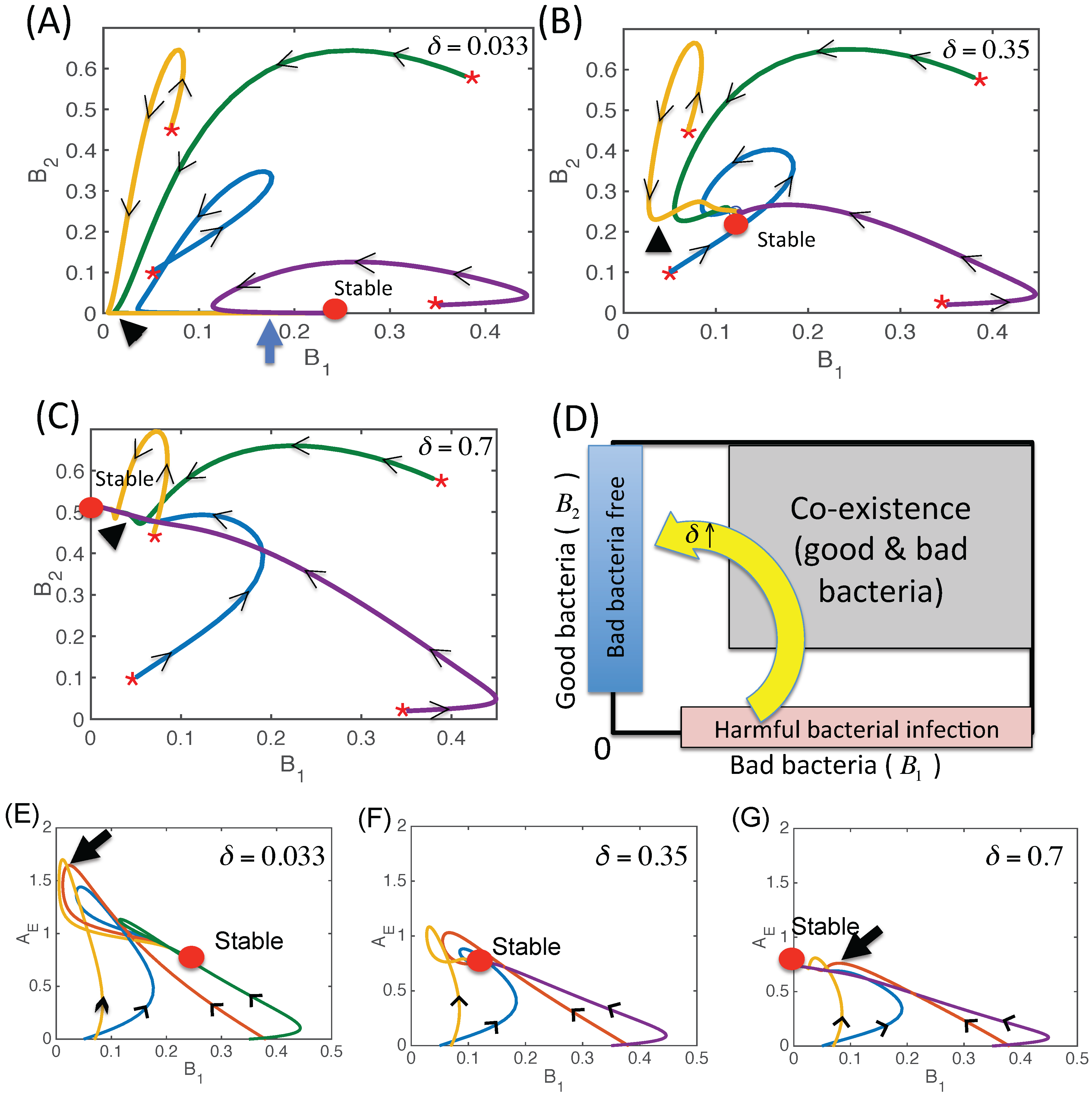
3.2.3. Dynamics of the Competition Model M2 in Response to the Immune System
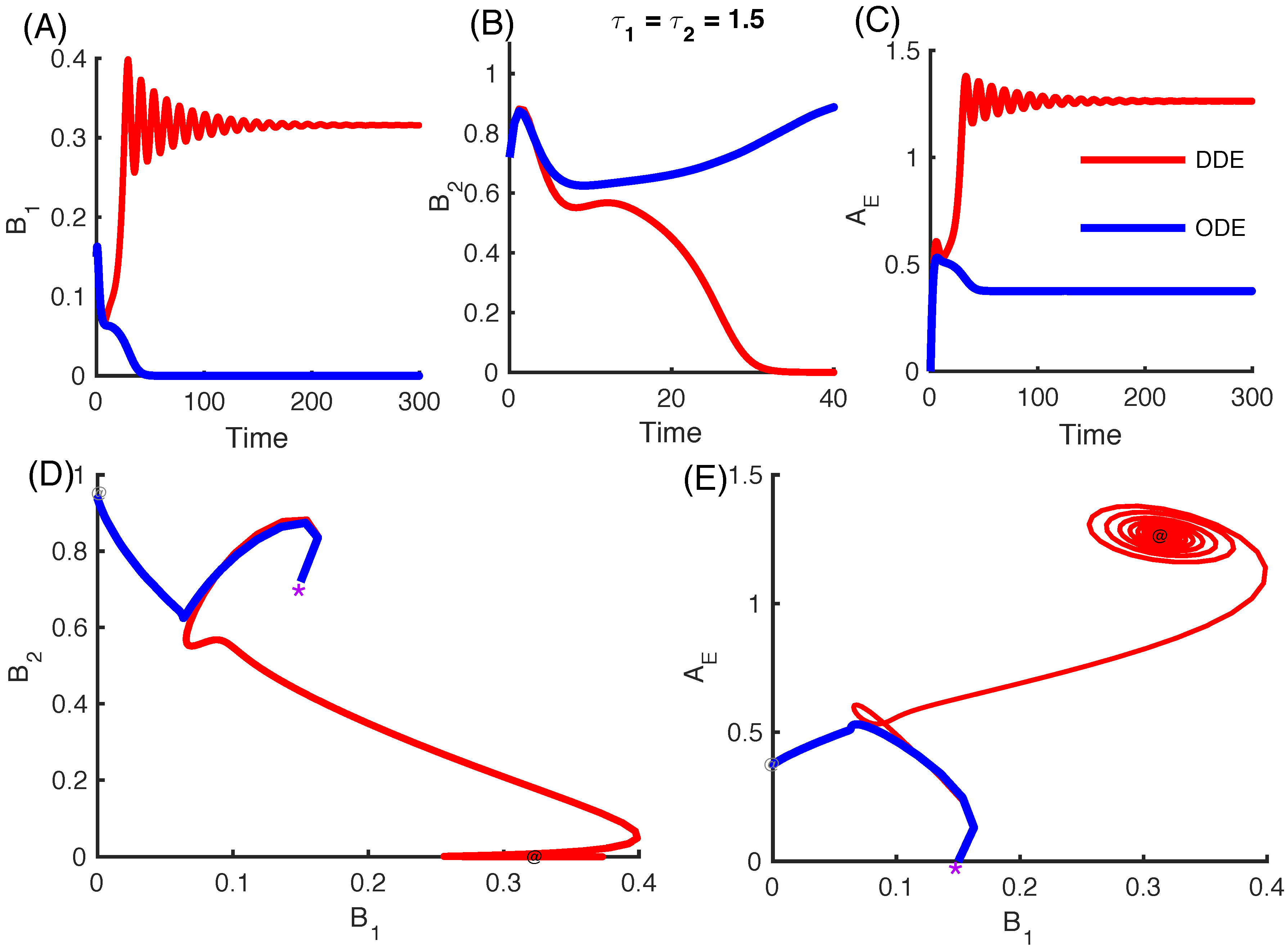
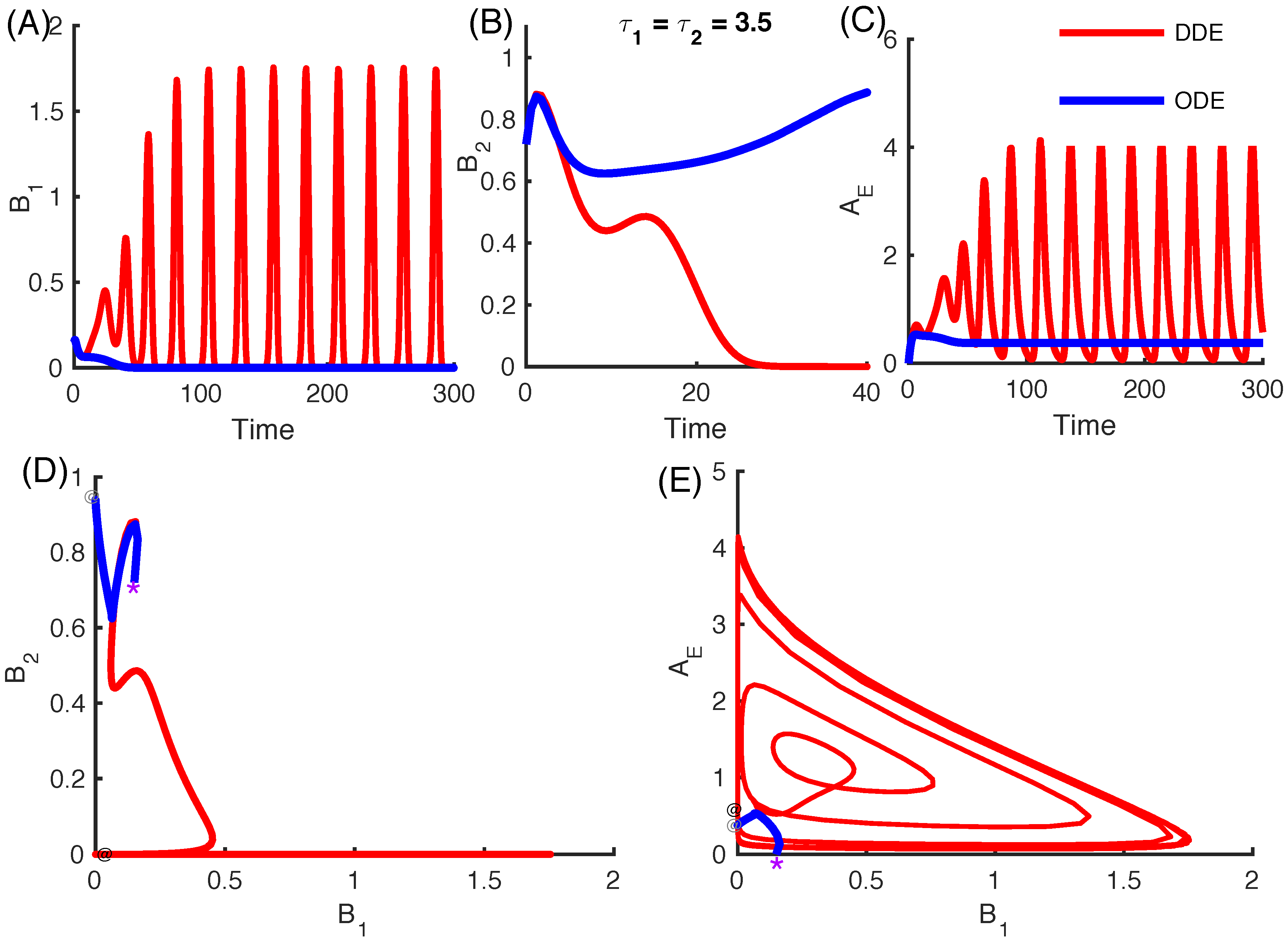
3.2.4. Effect of Time Delays in Immune Response on the Competition System
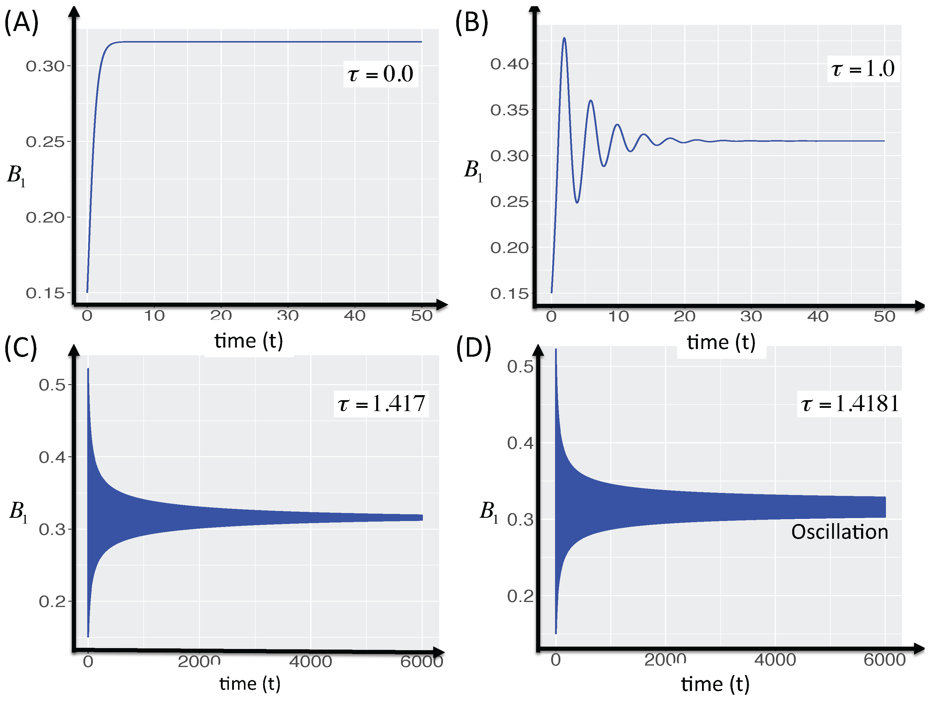
3.2.5. Local Stability Analysis of Delay Differential Equations
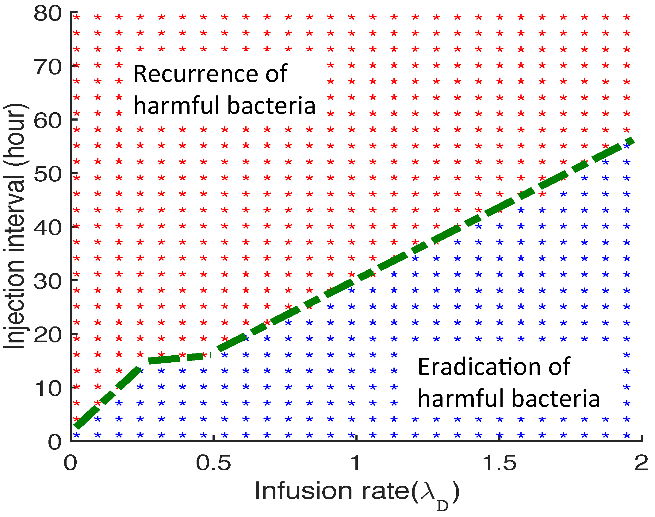
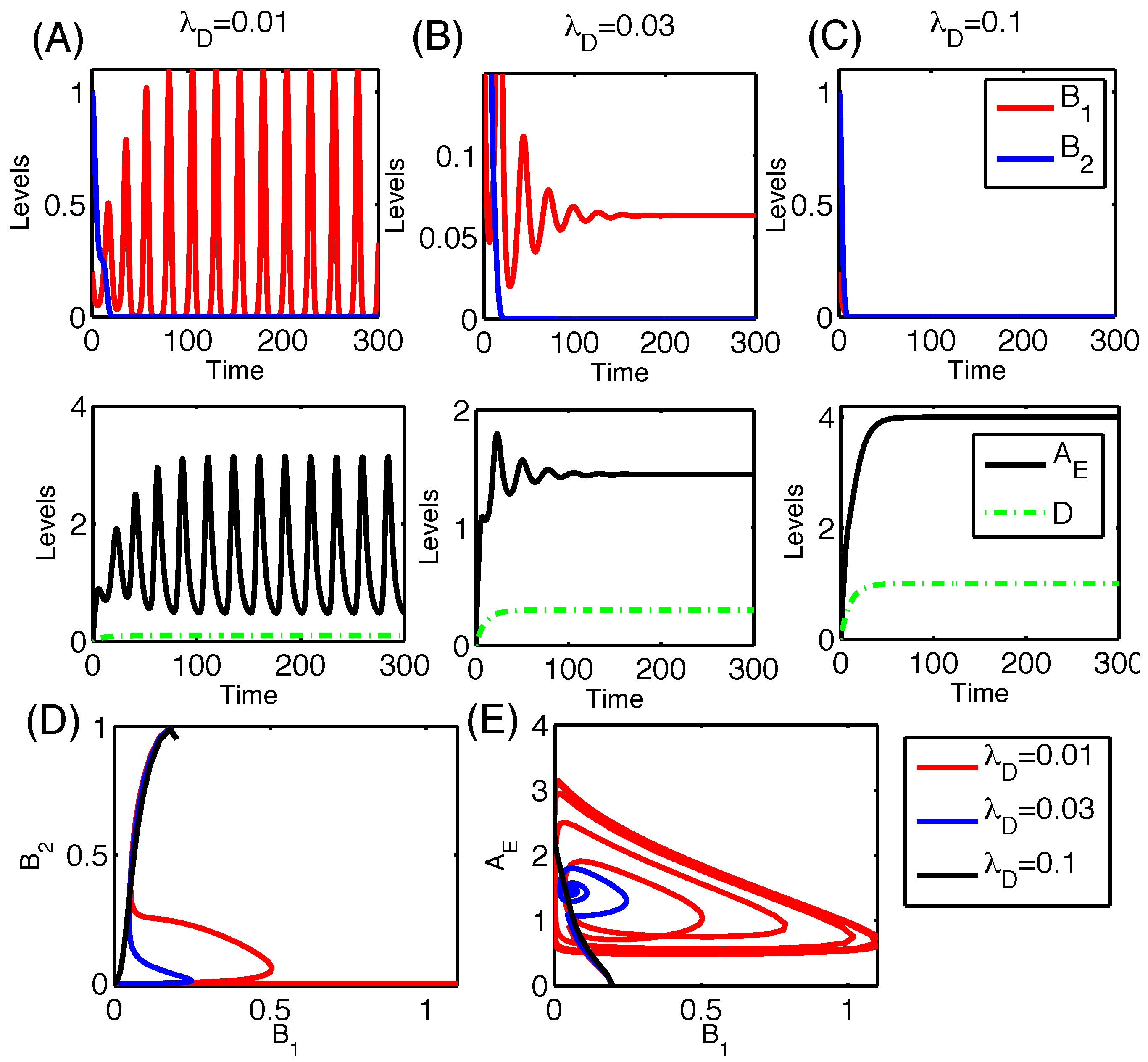
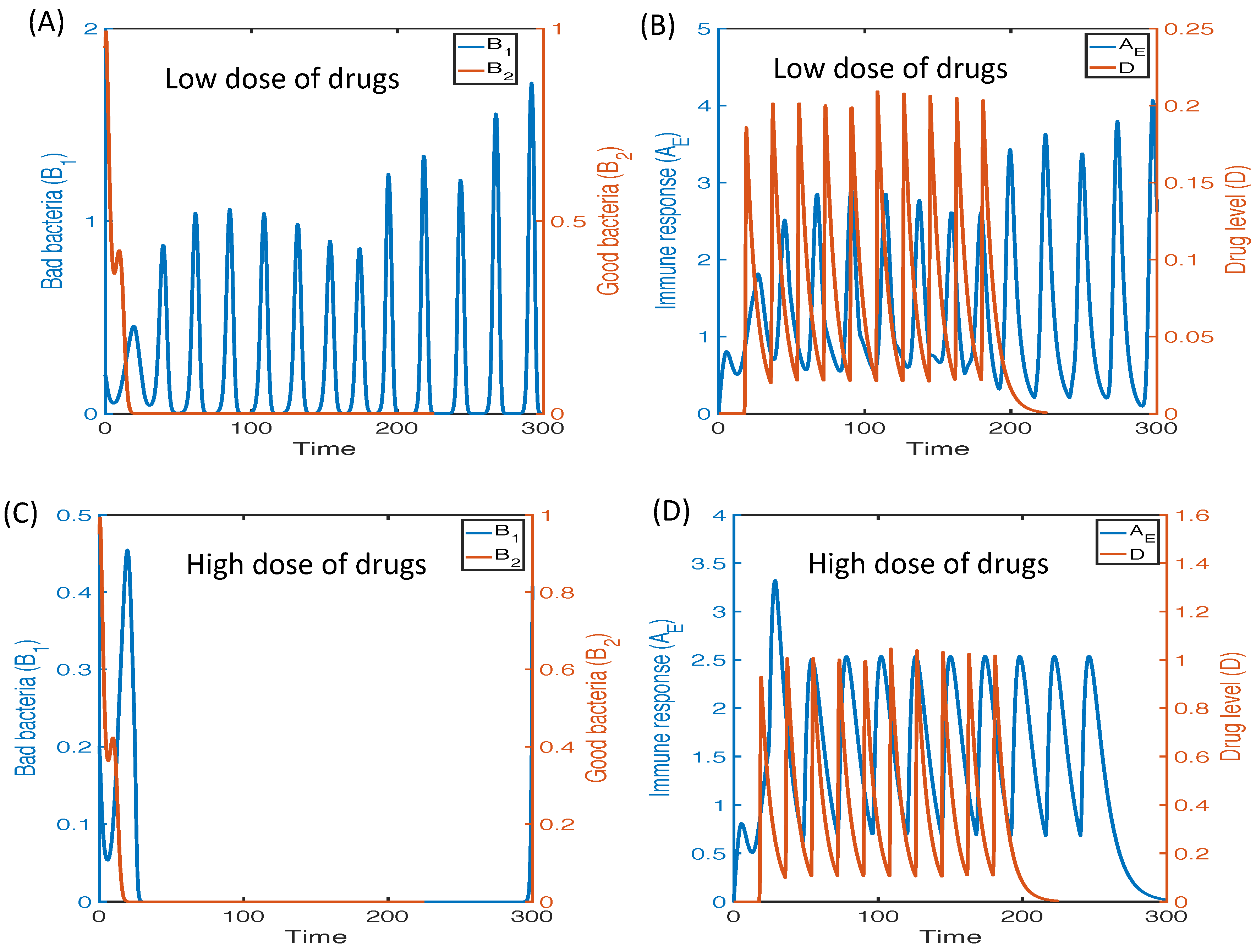
3.2.6. Therapeutic Approaches
4. Conclusions and Discussion
- In the present model, we concentrated on two major pathogenic and commensal bacterial species to obtain basic insight into how microbial interactions mediated chronic inflammation. However, more than hundreds of bacterial species have been demonstrated to coexist in the skin tissue. Metagenomic analysis targeting the gut- and skin-resident microbiome has revealed that numerous uncultured species exist and potentially affect the maintenance of skin homeostasis, as well as the progression of skin inflammatory disease [46]. The existence of spatial compartmentalization by forming heterogeneous clusters of colonies across the epidermis and dermis has been shown [47,48]. Although a few numbers of dominant species exist in terms of population abundance, bacterial diversity in the skin is highly maintained [49]. Complex interactions among commensal bacteria, the host immune system and different sources of environmental fluctuations should be essential factors for the maintenance of species diversity. Therefore, the incorporation of more than two bacterial species into the model would be more realistic. Colonization of harmful bacteria would be prevented by community-level resistance by a bacterial community. The incorporation of multiple species interactions will provide new insights on how the loss of bacterial diversity would lead to high inflammatory states.
- We considered the same time delays in the M2 model in this work. There exists the possibility of an immune escape mechanism, which might justify the use of different time delays. For instance, certain types of bacteria downregulate antigenicity when they invade tissue in order to escape from immune surveillance [50]. This would lead to a time delay in the activation of the immune system. Major extensions of the current model to include different time delays are warranted.
- The mathematical models presented here do not distinguish immune cell types, which are crucial to determine the difference between the epidermis and the GI tract. For instance, Langerhans cells are the major resident immune cell type that stays below the second layer of the stratum granulosum (below the tight junction) and captures the antigen. After capturing the antigen, Langerhans cells move to a draining lymph node to present the antigen to lymphocytes, known as homing. In the intestine, invading bacteria that attach to the gut epithelial cells trigger inflammatory responses, and finally, these bacteria are eliminated by immune cells recruited from the Payer’s patch or gastric mucosal lymphoid follicles.
- Explicit incorporation of spatial structure is essential to represent specific and unique information to the epidermis or the GI tract. In the present paper, however, we focused on the role of bacterial species to induce inflammatory responses rather than spatial structure, which forms specific and unique interactions among invading bacteria and immune cells. The ongoing project aims to incorporate spatial structure and heterogeneity in immune cell subtypes, but it is currently under investigation.
- The major signaling networks that control the intracellular regulation of transcriptional factor, proteases and protease inhibitors need to be addressed.
- The microenvironment also plays an important role in the regulation of epidermis and stem cell dynamics [51]. These include other immune cells, endothelial cells and stromal cells, such as fibroblasts, as well as growth factors secreted by these cells.
- Cell-mechanical regulations, such as actin and serum response factor, were also shown to transduce bio-physical cues from the microenvironment to control epidermal stem cell fate [52].
Acknowledgments
Author Contributions
Conflicts of Interest
Appendix A. Nondimensionalization

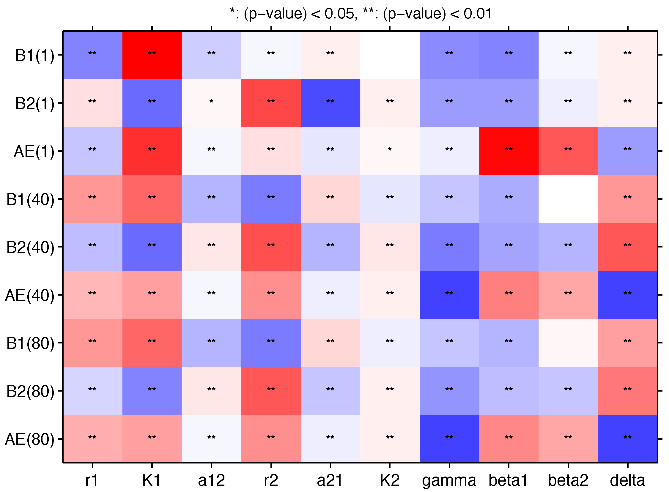
Appendix B. Sensitivity Analysis
| Par | γ | δ | ||||||||
|---|---|---|---|---|---|---|---|---|---|---|
| PRCC | ||||||||||
| −0.469 * | 0.9802 * | −0.206 * | −0.048 * | 0.0397 * | −0.0018 | −0.448 * | −0.464 * | −0.050 * | 0.0694 * | |
| 0.1245 * | −0.567 * | 0.0294 * | 0.6956 | −0.693 * | 0.0289 * | −0.399 * | −0.410 * | −0.060 * | 0.0541 * | |
| −0.237 * | 0.8100 * | −0.033 * | 0.1185 * | −0.114 * | 0.0091 | −0.093 * | 0.9596 * | 0.6476 * | −0.393 * | |
| 0.4098 * | 0.5636 * | −0.295 * | −0.500 * | 0.1479 * | −0.088 * | −0.248 * | −0.291 * | 0.0100 | 0.3772 * | |
| −0.264 * | −0.574 * | 0.0706 * | 0.6627 * | −0.292 * | 0.0687 * | −0.512 * | −0.384 * | −0.308 * | 0.6232 * | |
| 0.3034 * | 0.3626 * | −0.033 * | 0.4340 * | −0.082 * | 0.0782 * | −0.739 * | 0.4905 * | 0.3453 * | −0.743 * | |
| 0.4035 * | 0.5614 * | −0.292 * | −0.509 * | 0.1360 * | −0.085 * | −0.232 * | −0.284 * | 0.0212 | 0.3412 * | |
| −0.204 * | −0.478 * | 0.0704 * | 0.6061 * | −0.241 * | 0.0592 * | −0.406 * | −0.283 * | −0.247 * | 0.5178 * | |
| 0.3059 * | 0.3551 * | −0.031 * | 0.4312 * | −0.069 * | 0.0715 * | −0.728 * | 0.4730 * | 0.3195 * | −0.730 * | |
| Min | 0.5 | 0.1 | 0.1 | 0.1 | 0.1 | 1.0 | 0.1 | 0.05 | 0.05 | 0.01 |
| Base | 1.5 | 0.5 | 1.0 | 1.0 | 1.0 | 2.0 | 1.0 | 0.1 | 1.0 | 0.35 |
| Max | 2.5 | 2.5 | 2.0 | 2.0 | 2.0 | 2.5 | 2.0 | 2.0 | 2.0 | 1.0 |
References
- Chung, W.O.; Dale, B.A. Innate immune response of oral and foreskin keratinocytes: Utilization of different signaling pathways by various bacterial species. Infect. Immun. 2004, 72, 352–358. [Google Scholar] [CrossRef] [PubMed]
- Graham-Brown, R.; Burns, T. Lecture Notes: Dermatology, 10th ed.; Wiley-Blackwell: Hoboken, NJ, USA, 2011. [Google Scholar]
- Bieber, T. Atopic Dermatitis. N. Engl. J. Med. 2008, 358, 1483–1494. [Google Scholar] [CrossRef] [PubMed]
- Smith, F.J.D.; Irvine, A.D.; Terron-Kwiatkowski, A.; Sandilands, A.; Campbell, L.E.; Zhao, Y.; Liao, H.; Evans, A.T.; Goudie, D.R.; Lewis-Jones, S.; et al. Loss-of-function mutations in the gene encoding filaggrin cause ichthyosis vulgaris. Nat. Genet. 2006, 38, 337–342. [Google Scholar] [CrossRef] [PubMed]
- Kubo, A.; Nagao, K.; Amagai, M. Epidermal barrier dysfunction and cutaneous sensitization in atopic diseases. J. Clin. Investig. 2012, 122, 440–447. [Google Scholar] [CrossRef] [PubMed]
- Briot, A.; Deraison, C.; Lacroix, M.; Bonnart, C.; Robin, A.; Besson, C.; Dubus, P.; Hovnanian, A. Kallikrein 5 induces atopic dermatitis-like lesions through PAR2-mediated thymic stromal lymphopoietin expression in Netherton syndrome. J. Exp. Med. 2009, 206, 1135–1147. [Google Scholar] [CrossRef] [PubMed]
- Kobayashi, T.; Glatz, M.; Horiuchi, K.; Kawasaki, H.; Akiyama, H.; Kaplan, D.H.; Kong, H.H.; Amagai, M.; Nagao, K. Dysbiosis and Staphylococcus aureus Colonization Drives Inflammation in Atopic Dermatitis. Immunity 2015, 42, 756–766. [Google Scholar] [CrossRef] [PubMed]
- Tenover, F.C.; Pearson, M.L. Methicillin-resistant Staphylococcus aureus. Emerg. Infect. Dis. 2004, 10, 2052–2053. [Google Scholar] [CrossRef] [PubMed]
- Gallo, R.L.; Nakatsuji, T. Microbial symbiosis with the innate immune defense system of the skin. J. Investig. Dermatol. 2011, 131, 1974–1980. [Google Scholar] [CrossRef] [PubMed]
- Christensen, G.J.M.; Brüggemann, H. Bacterial skin commensals and their role as host guardians. Benef. Microbes 2014, 5, 201–215. [Google Scholar] [CrossRef] [PubMed]
- Prince, T.; McBain, A.J.; O’Neill, C.A. Lactobacillus reuteri protects epidermal keratinocytes from Staphylococcus aureus-induced cell death by competitive exclusion. Appl. Environ. Microbiol. 2012, 78, 5119–5126. [Google Scholar] [CrossRef] [PubMed]
- Murphy, K. Janeway’s Immunobiology, 8th ed.; Immunobiology: The Immune System (Janeway); Garland Science: New York, NY, USA, 2012. [Google Scholar]
- Shen, W.; Li, W.; Hixon, J.A.; Bouladoux, N.; Belkaid, Y.; Dzutzev, A.; Durum, S.K. Adaptive immunity to murine skin commensals. Proc. Natl. Acad. Sci. USA 2014, 111, E2977–E2986. [Google Scholar] [CrossRef] [PubMed]
- Nakamizo, S.; Egawa, G.; Honda, T.; Nakajima, S.; Belkaid, Y.; Kabashima, K. Commensal bacteria and cutaneous immunity. Semin. Immunopathol. 2015, 37, 73–80. [Google Scholar] [CrossRef] [PubMed]
- Thammavongsa, V.; Kim, H.K.; Missiakas, D.; Schneewind, O. Staphylococcal manipulation of host immune responses. Nat. Rev. Microbiol. 2015, 13, 529–543. [Google Scholar] [CrossRef] [PubMed]
- Lo, C.W.; Lai, Y.K.; Liu, Y.T.; Gallo, R.L.; Huang, C.M. Staphylococcus aureus hijacks a skin commensal to intensify its virulence: Immunization targeting β-hemolysin and CAMP factor. J. Investig. Dermatol. 2011, 131, 401–409. [Google Scholar] [CrossRef] [PubMed]
- Son, E.D.; Kim, H.J.; Park, T.; Shin, K.; Bae, I.H.; Lim, K.M.; Cho, E.G.; Lee, T.R. Staphylococcus aureus inhibits terminal differentiation of normal human keratinocytes by stimulating interleukin-6 secretion. J. Dermatol. Sci. 2014, 74, 64–71. [Google Scholar] [CrossRef] [PubMed]
- Schoenfelder, S.M.K.; Lange, C.; Eckart, M.; Hennig, S.; Kozytska, S.; Ziebuhr, W. Success through diversity—How Staphylococcus epidermidis establishes as a nosocomial pathogen. Int. J. Med. Microbiol. 2010, 300, 380–386. [Google Scholar] [CrossRef] [PubMed]
- Lai, Y.; Cogen, A.L.; Radek, K.A.; Park, H.J.; Macleod, D.T.; Leichtle, A.; Ryan, A.F.; Di Nardo, A.; Gallo, R.L. Activation of TLR2 by a small molecule produced by Staphylococcus epidermidis increases antimicrobial defense against bacterial skin infections. J. Investig. Dermatol. 2010, 130, 2211–2221. [Google Scholar] [CrossRef] [PubMed]
- Rizzo, A.; Losacco, A.; Carratelli, C.R.; Domenico, M.D.; Bevilacqua, N. Lactobacillus plantarum reduces Streptococcus pyogenes virulence by modulating the IL-17, IL-23 and Toll-like receptor 2/4 expressions in human epithelial cells. Int. Immunopharmacol. 2013, 17, 453–461. [Google Scholar] [CrossRef] [PubMed]
- Vergnolle, N. Protease inhibition as new therapeutic strategy for GI diseases. Gut 2016, 65, 1215–1224. [Google Scholar] [CrossRef] [PubMed]
- Biancheri, P.; Di Sabatino, A.; Corazza, G.R.; MacDonald, T.T. Proteases and the gut barrier. Cell Tissue Res. 2013, 351, 269–280. [Google Scholar] [CrossRef] [PubMed]
- Kim, Y.; Roh, S. A hybrid model for cell proliferation and migration in glioblastoma. Discret. Contin. Dyn. Syst. B 2013, 18, 969–1015. [Google Scholar] [CrossRef]
- Kim, Y.; Kang, H.; Powathil, G.; Kim, H.; Trucu, D.; Lee, W.; Lawler, S.; Chaplain, M. MicroRNA regulation of a cancer network in glioblastoma: The role of miR-451-AMPK-mTOR in regulation of cell proliferation and infltration. J. Roy. Soc. Interface 2015. submitted. [Google Scholar]
- Lee, S.; Hwang, H.; Kim, Y. Modeling the role of TGF-beta in regulation of the Th17 phenotype in the LPS-driven immune system. Bull. Math. Biol. 2014, 76, 1045–1080. [Google Scholar] [CrossRef] [PubMed]
- Lim, J.; Lee, S.; Kim, Y. Hopf bifurcation in a model of TGF-beta in regulation of the Th17 phenotype. Discret. Contin.s Dyn. Syst. B 2016, in press. [Google Scholar]
- Sato, M.; Hata, N.; Asagiri, M.; Nakaya, T.; Taniguchi, T.; Tanaka, N. Positive feedback regulation of type I IFN genes by the IFN-inducible transcription factor IRF-7. FEBS Lett. 1998, 441, 106–110. [Google Scholar] [CrossRef]
- Prassas, I.; Eissa, A.; Poda, G.; Diamandis, E.P. Unleashing the therapeutic potential of human kallikrein-related serine proteases. Nat. Rev. Drug Discov. 2015, 14, 183–202. [Google Scholar] [CrossRef] [PubMed]
- D’Elia, R.V.; Harrison, K.; Oyston, P.C.; Lukaszewski, R.A.; Clark, G.C. Targeting the “cytokine storm” for therapeutic benefit. Clin. Vaccine Immunol. 2013, 20, 319–327. [Google Scholar] [CrossRef] [PubMed]
- Castellarin, M.; Warren, R.; Freeman, J.; Dreolini, L.; Krzywinski, M.; Strauss, J.; Barnes, R.; Watson, P.; Allen-Vercoe, E.; Moore, R.; et al. Fusobacterium nucleatum infection is prevalent in human colorectal carcinoma. Genome Res. 2012, 22, 299–306. [Google Scholar] [CrossRef] [PubMed]
- Kostic, A.; Gevers, D.; Pedamallu, C.; Michaud, M.; Duke, F.; Earl, A.; Ojesina, A.; Jung, J.; Bass, A.; Tabernero, J.; et al. Genomic analysis identifies association of Fusobacterium with colorectal carcinoma. Genome Res. 2012, 22, 292–298. [Google Scholar] [CrossRef] [PubMed]
- Africa, C.; Nel, J.; Stemmet, M. Anaerobes and Bacterial Vaginosis in Pregnancy: Virulence Factors Contributing to Vaginal Colonisation. Int. J. Environ. Res. Public Health 2014, 11, 6979–7000. [Google Scholar] [CrossRef] [PubMed]
- Marteau, P. Bacterial Flora in Inflammatory Bowel Disease. Dig. Dis. 2009, 27, 99–103. [Google Scholar] [CrossRef] [PubMed]
- Lepage, P.; Leclerc, M.; Joossens, M.; Mondot, S.; Blottiere, H.; Raes, J.; Ehrlich, D.; Dore, J. A metagenomic insight into our gut’s microbiome. Gut 2012, 62, 146–158. [Google Scholar] [CrossRef] [PubMed]
- Lakhan, S.; Kirchgessner, A. Gut inflammation in chronic fatigue syndrome. Nutr. Metab. 2010, 7, 79. [Google Scholar] [CrossRef] [PubMed]
- Turnbaugh, P.; Ley, R.; Mahowald, M.; Magrini, V.; Mardis, E.; Gordon, J. An obesity-associated gut microbiome with increased capacity for energy harvest. Nature 2006, 444, 1027–1031. [Google Scholar] [CrossRef] [PubMed]
- Turnbaugh, P.; Hamady, M.; Yatsunenko, T.; Cantarel, B.; Duncan, A.; Ley, R.; Sogin, M.; Jones, W.; Roe, B.; Affourtit, J.; et al. A core gut microbiome in obese and lean twins. Nature 2009, 457, 480–484. [Google Scholar] [CrossRef] [PubMed]
- Mazmanian, S. Capsular polysaccharides of symbiotic bacteria modulate immune responses during experimental colitis. J. Pediatr. Gastroenterol. Nutr. 2008, 46, 11–12. [Google Scholar]
- Kamada, N.; Seo, S.U.; Chen, G.Y.; Núñez, G. Role of the gut microbiota in immunity and inflammatory disease. Nat. Rev. Immunol. 2013, 13, 321–335. [Google Scholar] [CrossRef] [PubMed]
- Kubica, M.; Hildebrand, F.; Brinkman, B.M.; Goossens, D.; Del Favero, J.; Vercammen, K.; Cornelis, P.; Schröder, J.M.; Vandenabeele, P.; Raes, J.; et al. The skin microbiome of caspase-14-deficient mice shows mild dysbiosis. Exp. Dermatol. 2014, 23, 561–567. [Google Scholar] [CrossRef] [PubMed]
- Schommer, N.N.; Gallo, R.L. Structure and function of the human skin microbiome. Trends Microbiol. 2013, 21, 660–668. [Google Scholar] [CrossRef] [PubMed]
- Pugliese, A.; Gandolfi, A. A simple model of pathogen-immune dynamics including specific and non-specific immunity. Math. Biosci. 2008, 214, 73–80. [Google Scholar] [CrossRef] [PubMed]
- Malka, R.; Shochat, E.; Rom-Kedar, V. Bistability and bacterial infections. PLoS ONE 2010, 5, e10010. [Google Scholar] [CrossRef] [PubMed]
- Tanaka, R.J.; Ono, M.; Harrington, H.A. Skin barrier homeostasis in atopic dermatitis: Feedback regulation of kallikrein activity. PLoS ONE 2011, 6, e19895. [Google Scholar] [CrossRef] [PubMed]
- Mares, C.A.; Ojeda, S.S.; Morris, E.G.; Li, Q.; Teale, J.M. Initial delay in the immune response to Francisella tularensis is followed by hypercytokinemia characteristic of severe sepsis and correlating with upregulation and release of damage-associated molecular patterns. Infect. Immun. 2008, 76, 3001–3010. [Google Scholar] [CrossRef] [PubMed]
- Hannigan, G.D.; Grice, E.A. Microbial ecology of the skin in the era of metagenomics and molecular microbiology. Cold Spring Harb. Perspect. Med. 2013, 3, a015362. [Google Scholar] [CrossRef] [PubMed]
- Naik, S.; Bouladoux, N.; Wilhelm, C.; Molloy, M.J.; Salcedo, R.; Kastenmuller, W.; Deming, C.; Quinones, M.; Koo, L.; Conlan, S.; et al. Compartmentalized control of skin immunity by resident commensals. Science 2012, 337, 1115–1119. [Google Scholar] [CrossRef] [PubMed]
- Belkaid, Y.; Naik, S. Compartmentalized and systemic control of tissue immunity by commensals. Nat. Immunol. 2013, 14, 646–653. [Google Scholar] [CrossRef] [PubMed]
- Grice, E.A.; Segre, J.A. The human microbiome: Our second genome. Annu. Rev. Genom. Hum. Genet. 2012, 13, 151–170. [Google Scholar] [CrossRef] [PubMed]
- Van Avondt, K.; van Sorge, N.M.; Sorge, N.M.V.; Meyaard, L. Bacterial immune evasion through manipulation of host inhibitory immune signaling. PLoS Pathog. 2015, 11, e1004644. [Google Scholar] [CrossRef] [PubMed]
- Nie, J.; Fu, X.; Han, W. Microenvironment-dependent homeostasis and differentiation of epidermal basal undifferentiated keratinocytes and their clinical applications in skin repair. J. Eur. Acad. Dermatol. Venereol. 2013, 27, 531–535. [Google Scholar] [CrossRef] [PubMed]
- Connelly, J.; Gautrot, J.; Trappmann, B.; Tan, D.; Donati, G.; Huck, W.; Watt, F. Actin and serum response factor transduce physical cues from the microenvironment to regulate epidermal stem cell fate decisions. Nat. Cell Biol. 2010, 12, 711–718. [Google Scholar] [CrossRef] [PubMed]
- Kim, Y.; Stolarska, M.; Othmer, H. A hybrid model for tumor spheroid growth in vitro I: Theoretical development and early results. Math. Models Methods Appl. Sci. 2007, 17, 1773–1798. [Google Scholar] [CrossRef]
- Kim, Y.; Stolarska, M.; Othmer, H. The role of the microenvironment in tumor growth and invasion. Prog. Biophys. Mol. Biol. 2011, 106, 353–379. [Google Scholar] [CrossRef] [PubMed]
- Kim, Y. Regulation of cell proliferation and migration in glioblastoma: New therapeutic approach. Front. Mol. Cell. Oncol. 2013, 3, 53. [Google Scholar] [CrossRef] [PubMed]
- Kim, Y.; Othmer, H. A hybrid model of tumor-stromal interactions in breast cancer. Bull. Math. Biol. 2013, 75, 1304–1350. [Google Scholar] [CrossRef] [PubMed]
- Kim, Y.; Powathil, G.; Kang, H.; Trucu, D.; Kim, H.; Lawler, S.; Chaplain, M. Strategies of eradicating glioma cells: A multi-scale mathematical model with miR-451-AMPK-mTOR control. PLoS ONE 2015, 10, e0114370. [Google Scholar] [CrossRef] [PubMed]
- Lee, M.H.; Arrecubieta, C.; Martin, F.J.; Prince, A.; Borczuk, A.C.; Lowy, F.D. A postinfluenza model of Staphylococcus aureus pneumonia. J. Infect. Dis. 2010, 201, 508–515. [Google Scholar] [CrossRef] [PubMed]
- Lin, R.; Kwok, J.; Crespo, D.; Fawcett, J. Chondroitinase ABC has a long-lasting effect on chondroitin sulphate glycosaminoglycan content in the injured rat brain. J. Neurochem. 2008, 104, 400–408. [Google Scholar] [CrossRef] [PubMed]
- Gu, W.; Fu, S.; Wang, Y.; Li, Y.; Lu, H.; Xu, X.; Lu, P. Chondroitin sulfate proteoglycans regulate the growth, differentiation and migration of multipotent neural precursor cells through the integrin signaling pathway. BMC Neurosci. 2009, 10, 1–15. [Google Scholar] [CrossRef] [PubMed]
- Bruckner, G.; Bringmann, A.; Hartig, W.; Koppe, G.; Delpech, B.; Brauer, K. Acute and long-lasting changes in extracellular-matrix chondroitin-sulphate proteoglycans induced by injection of chondroitinase ABC in the adult rat brain. Exp. Brain Res. 1998, 121, 300–310. [Google Scholar] [CrossRef] [PubMed]
- Kim, Y.; Lee, H.; Dmitrieva, N.; Kim, J.; Kaur, B.; Friedman, A. Choindroitinase ABC I-mediated enhancement of oncolytic virus spread and anti-tumor efficacy: A mathematical model. PLoS ONE 2014, 9, e102499. [Google Scholar] [CrossRef] [PubMed]
- Milo, R.; Phillips, R. Cell Biology by the Numbers, 1st ed.; Taylor & Francis: Philadelphia, PA, USA, 2015; ISBN 9780815345374. [Google Scholar]
- Kim, Y.K.; Oh, S.Y.; Jeon, S.G.; Park, H.W.; Lee, S.Y.; Chun, E.Y.; Bang, B.; Lee, H.S.; Oh, M.H.; Kim, Y.S.; et al. Airway exposure levels of lipopolysaccharide determine type 1 versus type 2 experimental asthma. J. Immunol. 2007, 178, 5375–5382. [Google Scholar] [CrossRef] [PubMed]
- Kim, Y.; Lee, S.; Kim, Y.; Kim, Y.; Gho, Y.; Hwang, H.; Lawler, S. Regulation of Th1/Th2 cells in asthma development: A mathematical model. Math. Biosci. Eng. 2013, 10, 1095–1133. [Google Scholar] [PubMed]
- Marino, S.; Hogue, I.; Ray, C.; Kirschner, D. A methodology for performing global uncertainty and sensitivity analysis in systems biology. J. Theor. Biol. 2008, 254, 178–196. [Google Scholar] [CrossRef] [PubMed]
- Kirschner, D. Uncertainty And Sensitivity Analysis. Available online: http://malthus.micro.med.umich.edu/lab/usadata/ (accessed on 1 March 2016).


| Parameter | Description | Value |
|---|---|---|
| Maximum activation rate of proteases by TFs | 8–100 | |
| Half saturation constant of proteases by TFs | 3.0 | |
| Inhibitory strength of proteases activation by TFs | 1 | |
| n | Hill cooperativity coefficient | 2 |
| Maximum activation rate of proteases by bacteria | 8 | |
| Half saturation constant of proteases by bacteria | 3.0 | |
| Inhibitory strength of proteases activation by bacteria | 1 | |
| Maximum activation rate of TFs by proteases | 8 | |
| Half saturation constant of TFs by proteases | 3.0 | |
| Inhibitory strength of TF activation by proteases by | 1 | |
| Maximum activation rate of TFs by bacteria | 8 | |
| Half saturation constant of TFs by bacteria | 3.0 | |
| Inhibitory strength of TFs by bacteria | 1 | |
| Maximum activation rate of TFs by cytokines | 8 | |
| Half saturation constant of TFs by cytokines | 3.0 | |
| Inhibitory strength of TFs by cytokines | 1 | |
| Maximum activation rate of cytokines by TFs | 8 | |
| Half saturation constant of cytokines by TFs | 3.0 | |
| Inhibitory strength of cytokines by TFs | 1 | |
| Degradation rate of protease | 3.0 | |
| Degradation rate of transcription factor | 3.0 | |
| Degradation rate of extracellular cytokines | 3.0 | |
| λ | Migration rate of bacteria | 0.1 |
| Population growth rate of bacteria | 0.1 | |
| K | Carrying capacity of bacteria | 10.0 |
| γ | Per capita elimination rate of bacteria | 1.0 |
| Case | ||
|---|---|---|
| & | nonexistence | |
| & | ||
| & | nonexistence | nonexistence |
| & | nonexistence |
| Case | ||
|---|---|---|
| & | nonexistence | |
| & | nonexistence | nonexistence |
| & | ||
| & | nonexistence |
| Parameter | Description | Type I | Type II |
|---|---|---|---|
| Inter- and intra-competition | |||
| Inter-specific competition coefficient | |||
| Inter-specific competition coefficient | |||
| Intra-specific competition coefficient | 1.0 | 1.0 | |
| Intra-specific competition coefficient | 1.0 | 1.0 | |
| Activation/production rates | |||
| Growth rate of harmful bacteria | 1.5 | 1.5 | |
| Growth rate of good bacteria | 1.0 | 1.0 | |
| activation of cytokines by harmful bacteria | 0.1 | 1.0 | |
| activation of cytokines by good bacteria | 1.0 | 0.1 | |
| Inhibition/decay Rates | |||
| γ | Per capita elimination rate of bacteria | 1.0 | 1.0 |
| δ | Decay rate of cytokines | 0.35 | 0.25 |
© 2016 by the authors; licensee MDPI, Basel, Switzerland. This article is an open access article distributed under the terms and conditions of the Creative Commons Attribution (CC-BY) license (http://creativecommons.org/licenses/by/4.0/).
Share and Cite
Nakaoka, S.; Kuwahara, S.; Lee, C.H.; Jeon, H.; Lee, J.; Takeuchi, Y.; Kim, Y. Chronic Inflammation in the Epidermis: A Mathematical Model. Appl. Sci. 2016, 6, 252. https://doi.org/10.3390/app6090252
Nakaoka S, Kuwahara S, Lee CH, Jeon H, Lee J, Takeuchi Y, Kim Y. Chronic Inflammation in the Epidermis: A Mathematical Model. Applied Sciences. 2016; 6(9):252. https://doi.org/10.3390/app6090252
Chicago/Turabian StyleNakaoka, Shinji, Sota Kuwahara, Chang Hyeong Lee, Hyejin Jeon, Junho Lee, Yasuhiro Takeuchi, and Yangjin Kim. 2016. "Chronic Inflammation in the Epidermis: A Mathematical Model" Applied Sciences 6, no. 9: 252. https://doi.org/10.3390/app6090252
APA StyleNakaoka, S., Kuwahara, S., Lee, C. H., Jeon, H., Lee, J., Takeuchi, Y., & Kim, Y. (2016). Chronic Inflammation in the Epidermis: A Mathematical Model. Applied Sciences, 6(9), 252. https://doi.org/10.3390/app6090252