1. Introduction
The emergence of ultrafast ultrasound has been made possible by the development of new imaging modalities [
1,
2,
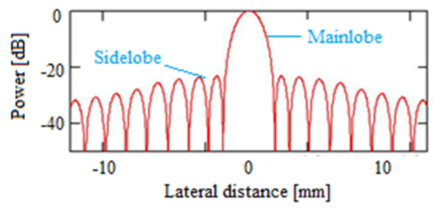
3]. Plane wave imaging (PWI) is a promising one which has attracted great attention. In the PWI, the entire region of interest (ROI) can be scanned using the full aperture in a single shot. Although plane waves enable covering a large field quickly, their imaging results have higher sidelobes compared with the conventional focused imaging. An example of sidelobes for a point target is given in
Figure 1. High sidelobes may lower imaging contrast [
4,
5] and make it difficult to detect the low scattering targets, such as small anechoic cysts. In the tissue characterization, high sidelobes may decrease the imaging resolution [
6].
Recently the concept of coherent plane wave compounding (CPWC) [
7] has been proposed to improve the imaging quality of the single-shot PWI. It has been proved that CPWC improves imaging lateral resolution and contrast-to-noise ratio (CNR) while still preserving a speed advantage over a focused linear-can acquisition [
8]. However, the sidelobes from different angles remain a problem and affect the imaging contrast.
In general, a sidelobe suppression method suitable for PWI demands rapidity. To date, few beamformers can meet this requirement [
9]. Generally, the sidelobe level can be reduced by applying apodization techniques, i.e., the Hamming window. However, the predefined weighting coefficients result in a wider mainlobe and thus reduce the lateral resolution which is intolerable in PWI. Adaptive beamformers [
10], such as the Capon beamformer or minimum variance (MV) beamformer [
11], have been proposed to compute the optimal weighting coefficients by using the information from the received raw channel data continually. Though effective for sidelobe rejection, this method also has several drawbacks for PWI. First, the computation load of the MV beamformer is intensive and not suitable in real-time processing [
12]. Second, the MV beamformer lacks robustness and artifacts can hardly be avoided [
13]. Other sidelobe suppression methods, such as dynamic focused reception, deconvolution, coherence weighting prior to the beam formation, and so on [
14,
15,
16], have also been suggested. Most of these methods have been proven capable of improving the contrast, but they all need additional intensive computation on the radio-frequency (RF) data and are not very suitable for PWI or CPWC.
In [
17], a singular value decomposition (SVD) filter is proposed for clutter rejection in Doppler and micro-bubble imaging. A set of frames sampled in a short time possesses the similar background signal which has high coherence. By using the SVD, researchers stripped out the high coherent component and left the flowing information. Inspired by this work, we introduce a new low-complexity sidelobe suppression beamformer applied to CPWC in this paper. It is the first time that the SVD filter is introduced in sidelobe suppression in PWI. In CPWC, the frames from different angles are analogous to a time series to some degree. As sidelobes from different angles are uncorrelated, a coherence-based SVD filter is adopted before the final coherent summation. For the sake of efficiency, the three-dimensional dataset is first transformed into a lower dimensional form, after which the computational increase is only related to the number of angles and acceptable for real-time imaging.
We assessed this new approach by simulation with the Field II program and phantom experiments with a Verasonics system on a commercial phantom. Results show that our method can reduce the sidelobes effectively with low additional computation. Additionally, its imaging quality including the lateral resolution is not affected compared to the original CPWC.
2. Materials and Methods
2.1. Coherent Plane Wave Compounding
In PWI, an image with poor quality is formed using backscattered echoes from a single shot [
18,
19]. In the CPWC mode, multiple plane waves are consecutively transmitted in different angles [
7]. Each transmission can be seen as a single-shot PWI.
Figure 2 illustrates the CPWC imaging scheme.
To transmit plane waves under different angles, transmit delays in the transducer need to be adjusted according to the formula:
where
represents the time delay for the element
i;
is the lateral coordinate of the element, with
being the coordinate of the leftmost and
being the coordinate of the rightmost transmitting element, respectively;
is the desired transmission angle; and
represents the speed of sound. These delays should also be considered when beamforming. In the simple CPWC, the beamformed data from all angles are summed and finally an image with the higher quality is obtained.
2.2. The Description of CPWC Acquisition
Inspired by [
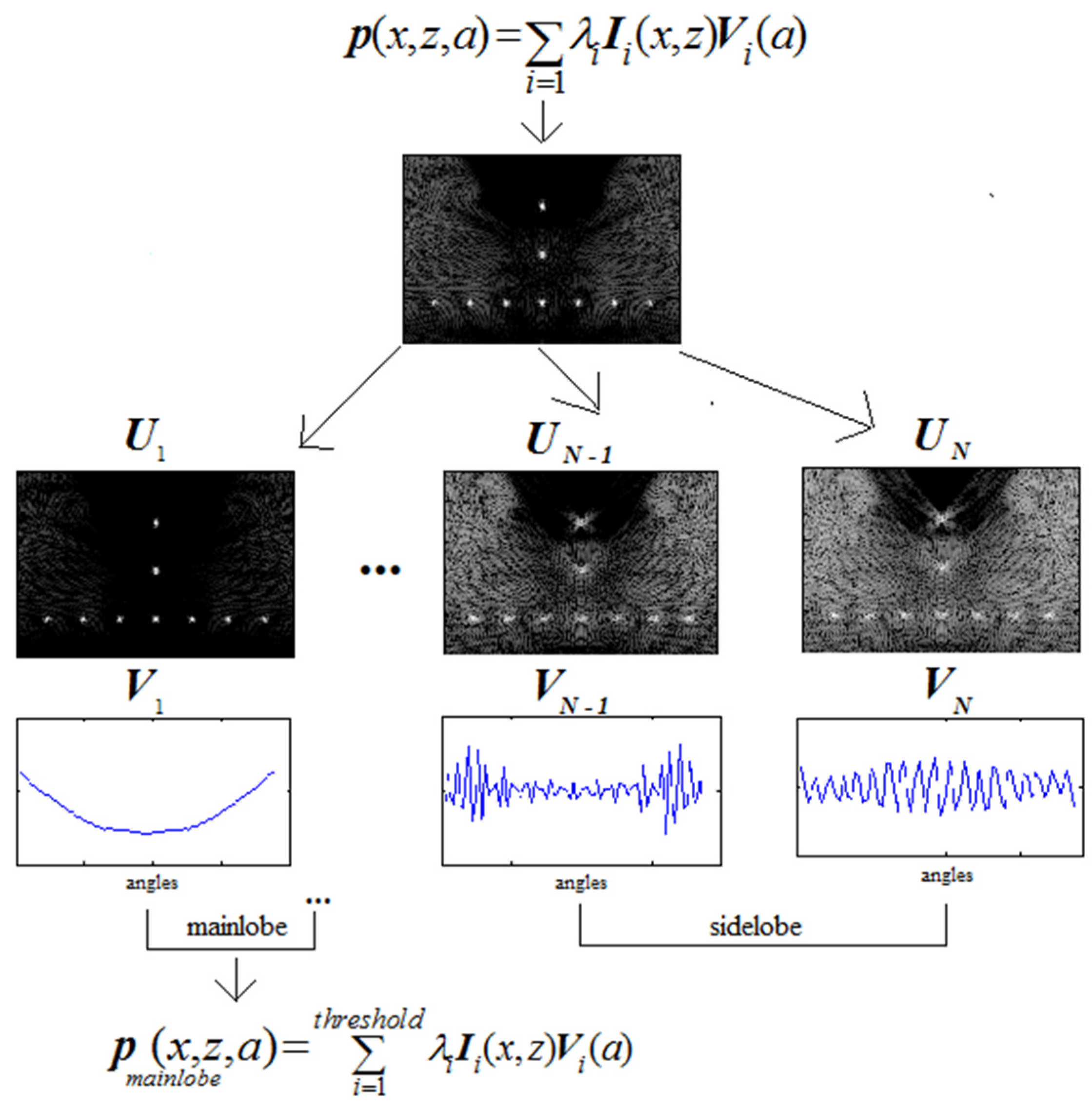
17], we represent the signal in a beamformed CPWC acquisition by a variable
, where
represents the lateral dimension,
represents the depth in the medium in front of the ultrasonic probe, and
represents the firing angle. It is assumed that this signal can be described as the summation of three contributions: the mainlobe signal
, the sidelobe signal
, and the electronic or thermal noise
:
Their contributions have different spatial and angular features. can be considered as a zero-mean Gaussian white noise. Sidelobes are closely related to the delays used for transmission, therefore, their spatial distribution becomes different among angles. From the perspective of the spatial coherence, from various has a rather weak correlation. On the contrary, the mainlobe energy originates from the on-axis target. Thus is almost identical within all acquisitions. Therefore, a separation method based on the covariance estimation certainly finds the highest covariance values for the mainlobe signal. This discrimination based on the covariance estimation can be performed by using the SVD of the beamformed RF data.
2.3. Singular Value Decomposition of CPWC Data
For one CPWC, there are
samples where
and
are the number of spatial samples along
x-direction and
z-direction, and
the number of angles. For the 3D dataset, dimension reduction is done first by transforming the angle sequence into a spatio-angular matrix
with dimensions
as shown in
Figure 3. This technique is common in processing time series [
17] or in other imaging modalities, such as computed tomography (CT) and magnetic resonance imaging (MRI) [
20,
21,
22,
23,
24], but it is rarely used in angle compounding.
The SVD of the matrix
is then used to find decomposition matrices, such as:
where
is a diagonal matrix with dimension
,
are the sorted singular values inside
,
and
are orthonormal matrices with respective dimensions
and
,
and
are the
ith columns of
and
, respectively, and
stands for the conjugate transpose.
Note that each column
corresponds to a spatial signal with the length of
which describes, in fact, a 2D spatial image
with dimensions
and each column
corresponds to an angular signal with the length of
. From this perspective, the SVD of
decomposes the field into a sum of separable images
, each characterized by a vector
, that are independently modulated by an angular signal
. Thus, owing to the SVD processing, the spatio-angular signal corresponding to ultrasonic beamformed RF data can be rewritten as:
Additionally, we can draw the conclusion that mainlobe components should be found mainly in the first singular values and singular vectors since their high spatio-angular coherence ensures the on-axis spatial pixels to exhibit the same angle profile. On the contrary, sidelobe signals should be described in the last singular values and singular vectors as they exhibit much lower spatio-angular coherence. Based on this, the sidelobe rejection is performed adaptively by using a threshold
on the number of singular vectors left from the original signal:
The graphical explanation of this SVD filter is shown in
Figure 4.
2.4. Implementation of SVD Filter with Low Complexity
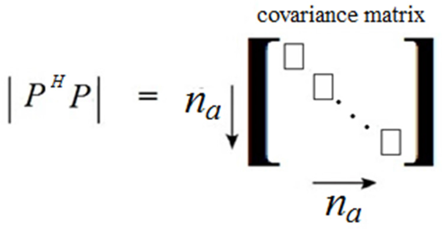
Considering the high dimension of
, directly applying the SVD is time-consuming and not suitable for real-time use. Analogous to the ultrafast time series, the CPWC acquisitions present a lot more spatial points (typically several 10,000) than angles (less than 100) in most cases. Thus, it can be less demanding to get the
covariance matrix as shown in
Figure 5 and diagonalize it from the point of view of computing. One should also notice that
and
also correspond to the eigenvectors of the respective covariance matrices
and
. Thus, this process can successfully reduce the
realizations of mainlobe spatial signals to a much smaller scale and get the angular eigenvectors that are also the right singular vector
of
. The weighted spatial vector
can be computed by the projection
then as Equation (6):
where
is the filtered dataset and
is a matrix filter defined by
, namely, a diagonal identity matrix with zeros for the last diagonal elements, leading to a new diagonal matrix
of singular values corresponding to the removal of the sidelobe and noise components. In this way, the computation load of the SVD filter is kept low and suitable for real-time imaging.
2.5. Coherent Summation with Filtered Frames
After the coherence-based filtering, the beamformed dataset should be transformed back to the compounding frames. Then the final imaging frame is obtained by the coherent summation of the filtered frames:
where
represents the summed result and
is the SVD-filtered frame.
To sum up, the SVD filter processes the intermediate results between the initial beamforming process and the final coherent compounding. It needs no other information and acts as a natural step in CPWC. Thus, the whole imaging process can be seen as an improved version of CPWC which inherits the merits of the original method.
2.6. Simulation and Phantom Experiment Setups
Experiments were devised to verify the effectiveness of our algorithm on sidelobe suppression by simulated and phantom experimental data. Several parameters related to the sidelobe level, resolution, and contrast were measured during the experiment.
2.6.1. Simulated Study
The simulated data were acquired with the commonly used ultrasound simulation tool Field II (Technical University of Denmark, Lyngby, Denmark) [
25]. The experimental setup for the simulation is shown in
Table 1.
We simulated a set of point targets in a homogeneous medium and an 8 mm radius anechoic cyst in a speckle pattern. An attenuation coefficient of 0.5 dB/(MHz·cm) has been simulated in order to mimic the properties of the phantom used for experiments.
In all simulations, plane waves with different steering angles were emitted. We selected an
F-number of 1.75 as in [
7]. The corresponding angle span [
,
] covered by the plane wave sequence is then given as:
The maximum number of plane waves
in the sequence is computed as:
where
and
are the aperture size and the wavelength respectively. In order to have an odd number of plane waves, we decided to transmit 75 steered plane waves regularly spaced between
and
for the acquisition of each phantom, which corresponds to an angle increment of 0.43°. No apodization is adopted for transmission. In our simulation, we picked out 11 angles uniformly from the 75 total angles for obtaining a good sidelobe suppression result in real-time.
2.6.2. Phantom Experiment
All phantom data were acquired using a commercially calibrated general-purpose multi-tissue phantom (Model 040GSE, Computerized Imaging Reference Systems Inc., Norfolk, VA, USA), using a Verasonics research scanner (Verasonics Corporation, Kirkland, WA, USA) with channel-domain data acquisition capabilities. In the phantom study, a commercial L11-4v transducer from Verasonics (Verasonics Corporation, Kirkland, WA, USA) was used. The parameters for the transducer and other experimental setups can also be found in
Table 1. The transmitting steering angle range was also from −16° to 16° (at 0.43° intervals; a total of 75 angles). No apodization is adopted for transmission. We also picked out 11 among the 75 total angles uniformly for the image reconstruction in the phantom experiment.
For both the simulation and the phantom experiment, the algorithms at the receiver end are implemented in MATLAB (Natick, MA, USA). All beamformers were performed on a standard desktop PC with an Intel (Santa Clara, CA, USA) Xeon CPU E5-2637 v2 3.50 GHz with 64 GB of RAM. The delay and sum (DAS) beamformer is adopted for the dynamic focus after a certain apodization if needed. In our SVD filter, only the first eigenvector is left for the mainlobe in both the simulation and the phantom experiment. In other words, and .
2.6.3. Test Parameters
We use the full-width at half-maximum (FWHM) and peak sidelobe (PSL), defined as the peak value of the first side lobe, to quantify the performance of beamformers for point targets. The former corresponds to the lateral resolution and the latter corresponds to the sidelobe level. For the anechoic cyst, we use both the contrast ratio (CR) and the CNR to evaluate the performance. The CR is defined as the ratio of the mean value in the background to the mean value in the cyst region [
26], and the CNR is defined as the CR divided by the standard deviation of the image intensity in the background region [
27].
3. Results
In this section, we will show the results of different beamforming schemes for the coherent plane wave dataset. Both simulation and phantom data are studied.
3.1. Simulated Study
3.1.1. Point Spread Function
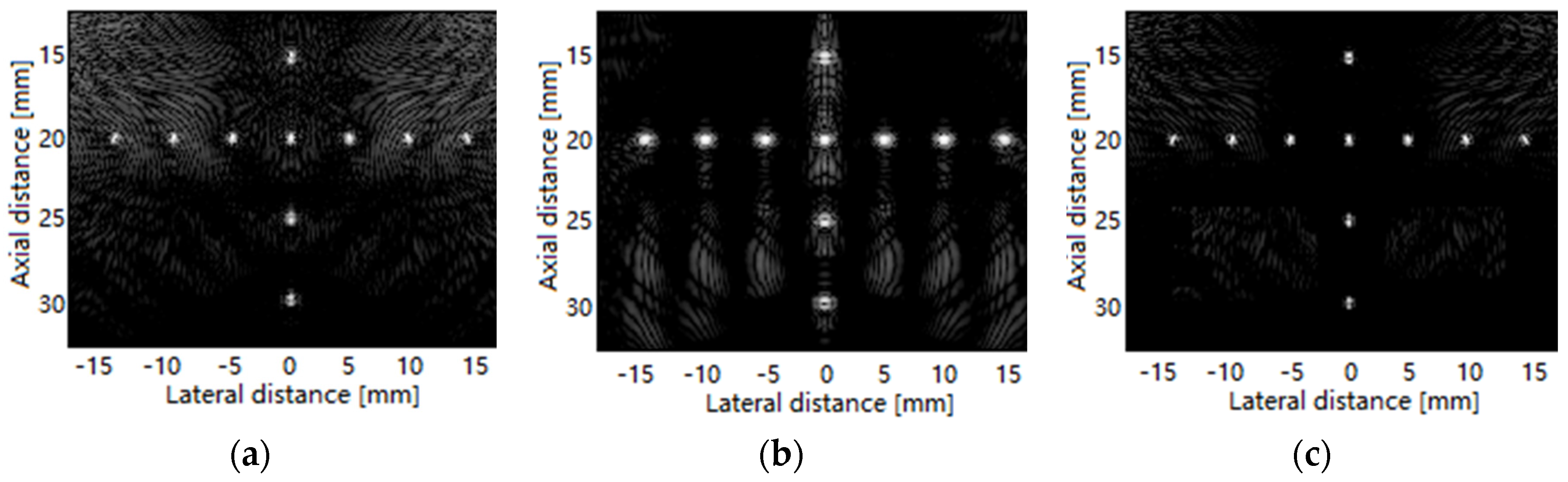
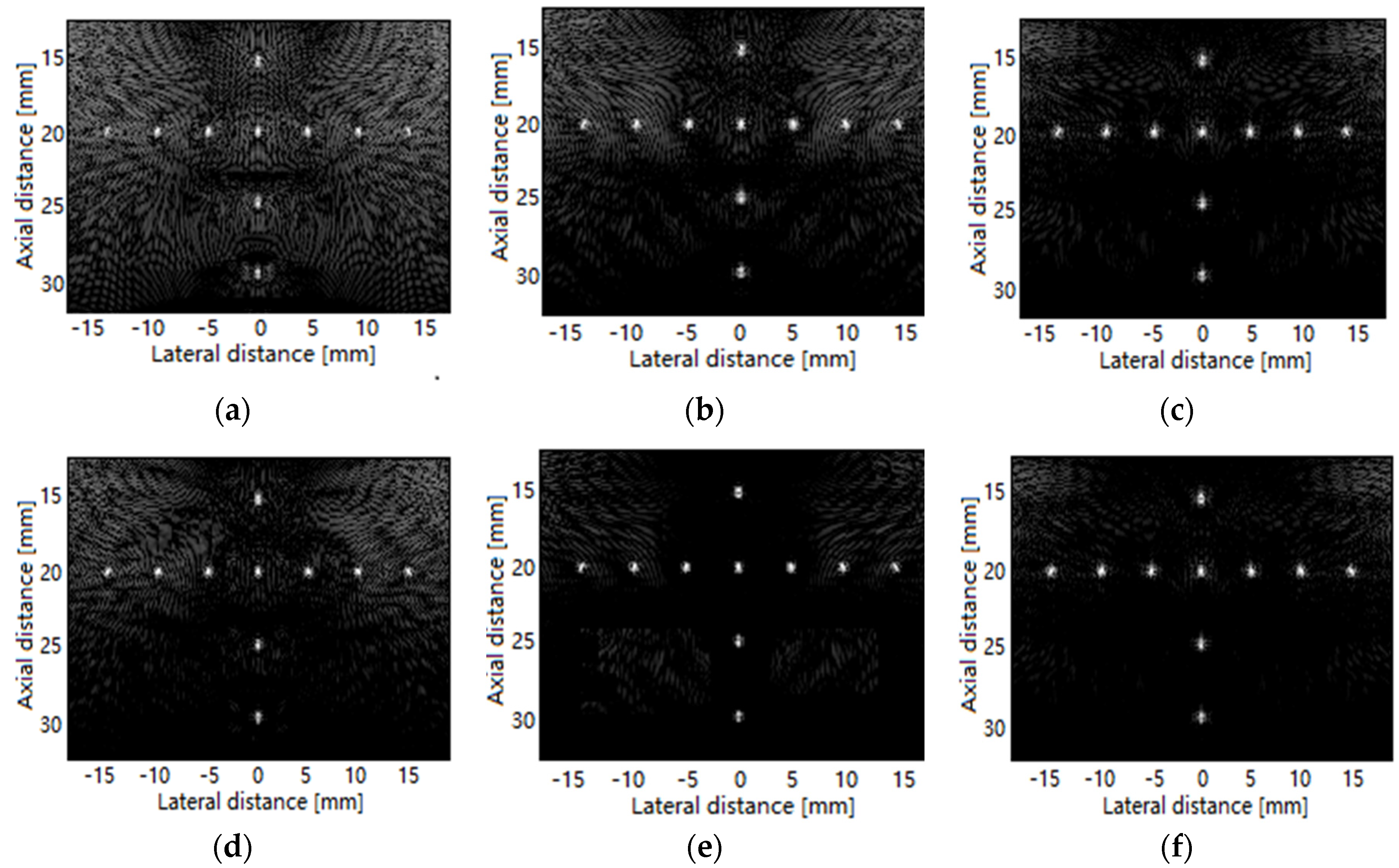
Figure 6 shows the beamformed responses of 10 point targets located at depths 15–30 mm using CPWC and our CPWC + SVD method over a 60 dB display dynamic range. As seen from
Figure 6a, the simple CPWC mode has high sidelobes. Although the sidelobe artifacts in the upper area are suppressed by the Hamming apodization, the artifacts at the bottom are strengthened in
Figure 6b. Meanwhile, the Hamming window apodization enlarges the mainlobe and lowers the lateral resolution. We also see from
Figure 6c that the proposed beamformer presents the same resolution as CPWC, and much better performance in terms of the sidelobe level.
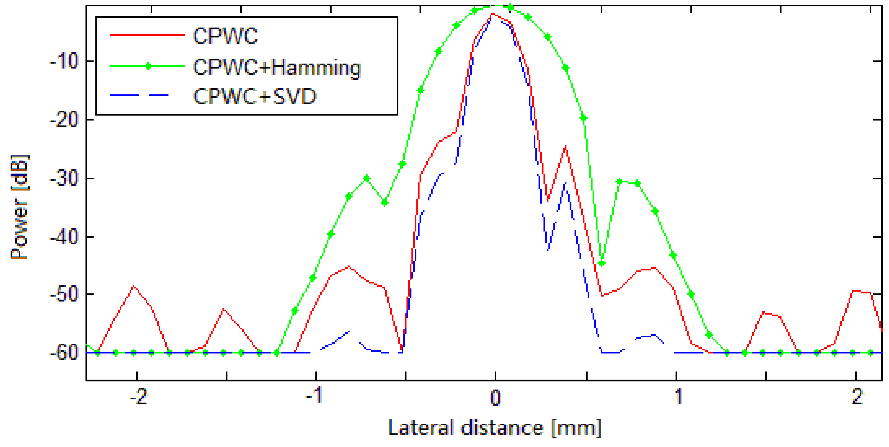
Figure 7 shows the lateral variation of beamformed responses of simulated point spread function (PSF) and confirms these qualitative observations. The target here is the central point located at the depth
z = 20 mm. As the results show, the proposed beamformer presents the same narrow mainlobe and lower sidelobe levels, with respect to CPWC. In terms of sidelobe levels, the first side level of the proposed beamformer is about 6.2 dB lower than that of CPWC. Combined with the Hamming window, CPWC loses its advantage in resolution. Specifically, the width of the mainlobe almost doubles.
The quantitative results of the FWHM and PSL are given in
Table 2. While the FWHMs of CPWC and CPWC + SVD are nearly the same, our method obtains a sidelobe 6 dB lower than CPWC, which indicates its validity for sidelobe suppression with respect to point targets in a homogeneous medium. Apodization has a similar performance as CPWC + SVD in the PSL, but its effect for the FWHM is serious.
3.1.2. Circular Anechoic Cyst in Speckle
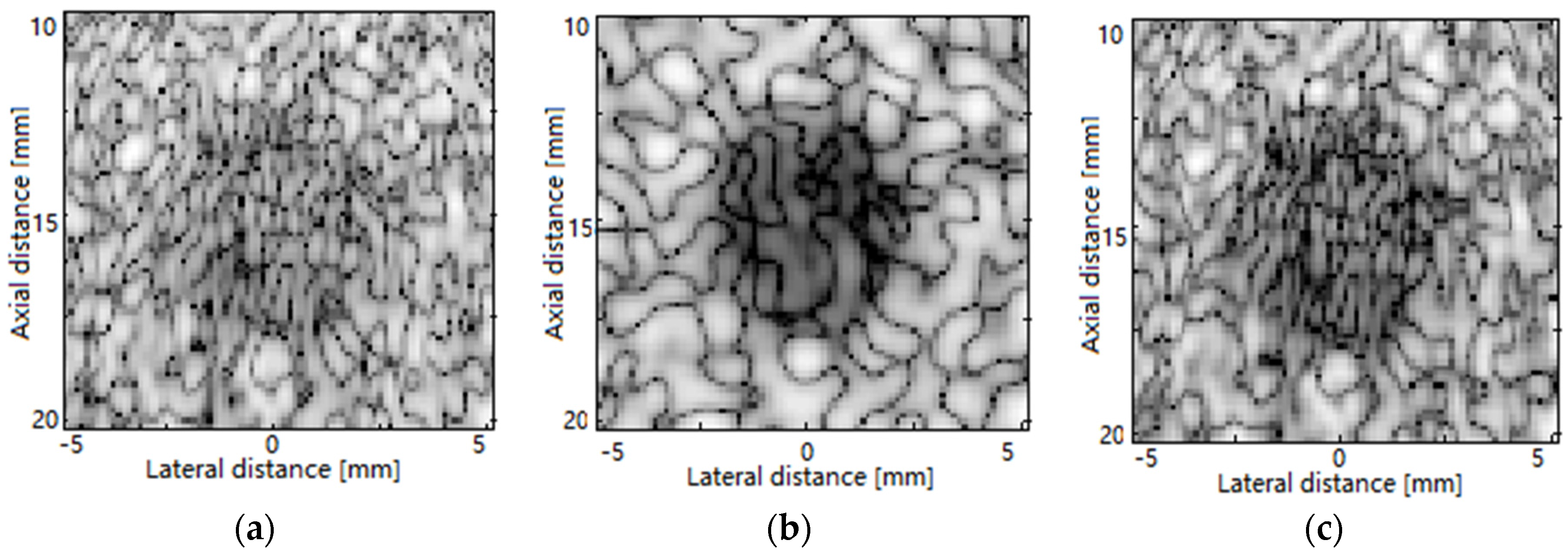
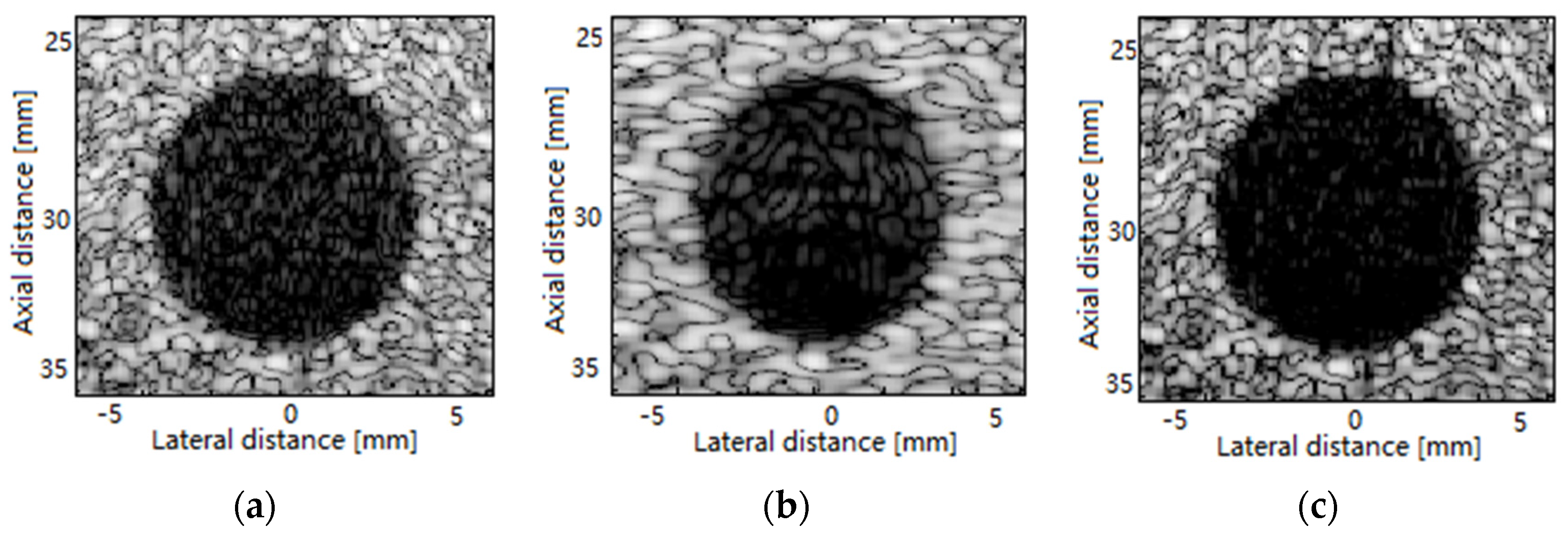
Figure 8 shows the beamformed images of a simulated 8 mm radius cyst using the CPWC and our CPWC + SVD method over a 60 dB display dynamic range. From
Figure 8 it can be observed that the proposed beamformer has an improvement over CPWC, which indicates the effectiveness of our coherence-based method for cysts. The window-weighted CPWC also has a better performance in terms of contrast, but the details are obscured due to the low resolution. To compute the mean values in the cyst region and in the background, we considered two circles with diameters of 4 and 6 mm, located at 30 mm in the depth, and 0 and 6 mm in the lateral direction, respectively.
Table 3 lists the relative CR and CNR for all beamforming methods. As seen, the performance of the proposed beamformer is significantly better in terms of both CR and CNR than the CPWC performance. Specifically, the proposed beamformer offers the contrast enhancement of 5.6 dB and improvement of CNR of about 12% in comparison to CPWC. CPWC + SVD also outperforms CPWC with Hamming apodization in CR and CNR.
3.2. Phantom Experiment
3.2.1. Point Target Phantom
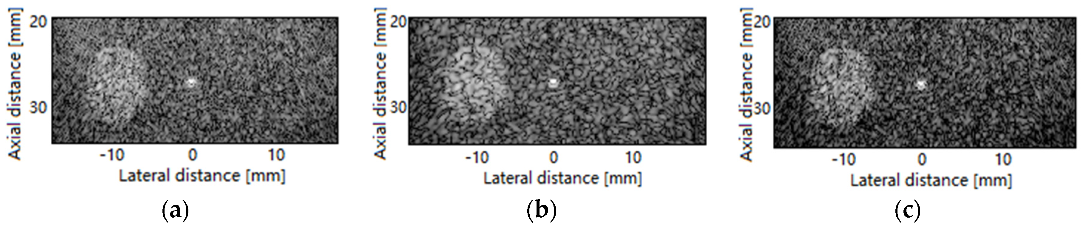
In the point target phantom, there is a point at 0.28 mm and a hyperechoic region with a radius of 4 mm.
Figure 9 shows the beamformed images of this complex scenario from depths 20–35 mm using CPWC, CPWC with Hamming apodization, and our CPWC + SVD method over a 60 dB display dynamic range. The performance of our algorithm is still robust in this situation. It can be seen in
Figure 9 that the proposed method maintains the mainlobe with the same width as CPWC. To compute the mean values in the hyperechoic region and in the background, we considered two circles with diameters of 4 and 6 mm, located at −10 and 10 mm in the lateral direction, respectively.
Table 4 gives the quantitative results. While the parameters of the resolution are near equal in CPWC and our CPWC + SVD method, our proposed beamformer can find an improvement of 2.6 dB in CR due to the sidelobe reduction outside the hyperechoic region. Compared to the Hamming CPWC, our beamformer shows a small contrast improvement due to the better sidelobe suppression ability.
3.2.2. Cyst Phantom
Figure 10 shows the beamformed images of a 4 mm radius cyst located at the depth of 15 mm using three methods over a 60 dB display dynamic range. In
Figure 10, it can be seen that the proposed method has better performance than the simple compounding method. This is due to the successful suppression of the sidelobe from the surrounding speckle.
Table 5 gives the quantitative data to better illustrate the performances. To compute the mean values in the cyst region and in the background, we considered two circles with diameters of 3 and 5 mm, located at 0 and 4 mm in the lateral direction, respectively. As seen in
Table 5, our coherence-based filter beamformer achieves an improvement of 5.7 dB over the simple CPWC in terms of CR. The corresponding enhancement reflected in CNR is above 20%. Two improved CPWC beamformers have obtained close results for contrast under this condition while ours performs better in the details inside and outside the cyst.
3.3. Algorithm Run Time
To verify the efficiency of our algorithm, we recorded the program run time in MATLAB (Natick, MA, USA). The total time contains the time for the receiving dynamic focus using DAS and the time for side lobe suppression. The experiments were repeated five times and the average results are given in
Table 6. As seen, the differences between the three beamformers are not significant. An increase within 0.2 s resulting from our algorithm is not obvious in comparison with the previous DAS process. Roughly, the difference between CPWC + SVD and CPWC can be seen as the time for the SVD filter. The results also show that the run time of our SVD filter is not affected by the imaging scenario or the region size.
3.4. Angle Selection
To further investigate the effect of angle quantity in our algorithm, five angles and 21 angles were selected for the PSF simulation as well. The beamformed results are shown in
Figure 11. As seen, fewer or more angles have more of an impact on plain CPWC results, as shown in
Figure 11a–c. The performances of our algorithm in
Figure 11d–f remain good and change little when increasing or decreasing the number of angles exploited for the image formation. Results shown in
Figure 11b,d and 11c,e are both comparable. This indicates that our algorithm is able to reach a similar performance as the simple CPWC using only half the angles.
Table 7 gives the run time for the above trials. In order to see the time for SVD filtering more clearly, we separate the total time into time for receiving dynamic focus and time for our sidelobe suppression. As
Table 7 shows, run time for our SVD filter grows almost cubically along with the increase of total angles. Combined with the results shown in
Figure 11, a similar imaging quality as the simple CPWC can be obtained faster by our SVD filter using fewer angles. Considering the competitive imaging performance, our algorithm is more suitable for a small angle number in real-time applications. A choice, like 11, in our experiment seems reasonable.
4. Discussion
The results of CPWC and CPWC + SVD applied to the simulated and the phantom data have been presented. From the results, we can see that the proposed method is useful in achieving a better performance than the traditional compounding method in terms of the sidelobe suppression and contrast enhancement. Compared to the traditional sidelobe suppression methods, our approach has two main advantages:
First, the proposed coherence-based method does not affect the lateral resolution as the apodization methods do. Our CPWC + SVD method is conducted on the receiver end after the DAS without manipulation of the waveform. Then, the coherence filter only removes the sidelobe and the noise among the CPWC frames, adaptively. Thus, the mainlobe is preserved during our process. Note that we chose 1 as the number of eigenvalues or eigenvectors in the adaptive filtering. This is due to our wish to reduce the sidelobe as much as possible.
Second, the contrast enhancement of the adaptive beamforming methods, such as the MV beamformer, comes at the cost of an extra computational load, which is too heavy for the plane wave imaging and CPWC. Suppose
l is the subarray length, the MV has the complexity O(
) by using Gaussian elimination for one covariance matrix inversion [
28]. For each angle, the matrix inversion process should repeat (
L-l) times for all subarrays. For
and
, the MV requires
floating operations in addition. However, the additional computation of our algorithm is relatively acceptable. As we know, the main computational amount occurs on the SVD of the covariance matrix. Since the matrix is a square matrix, the SVD equals the eigen-decomposition. The eigen-decomposition of the covariance matrix requires
floating operations by using the Golub-Reinsch algorithm [
29]. In other words, the computational amount is proportional to the cube of the angle number. Taking our experiments with 11 angles as an example, it will only require
floating operations in addition. The lack of an additional artifact is also an advantage of CPWC + SVD over the MV.
Aside from PWI, our proposed beamformer can also be used in the synthetic aperture (SA) imaging method since the SA is conceptually similar to CPWC [
30,
31]. In the SA method, RF data are obtained from pulse-echo sensing events of multiple point source firings at different lateral positions which are similar to the firings from different angles in CPWC. Broadly speaking, CPWC + SVD may be combined with other ultrasound imaging modes with several different firings.
5. Conclusions
This paper describes a new adaptive optimum beamformer for sidelobe reduction in plane wave compounding. The 3D compounding dataset is first transformed into a 2D spatio-angular matrix. Frames from different angles are then filtered by a coherence-based SVD filter accordingly and are summed to get the final result with better contrast. Simulation and experimental results demonstrate that the proposed sidelobe suppression beamforming technique may be used to improve the contrast of B-mode ultrasound images effectively.
In this method, a SVD filter is fitted into CPWC and the whole process can be viewed as an improved version of CPWC. We creatively apply the SVD filter to the angular domain via analogy. The transformation of the operating domain would be a highlight for the future use of the SVD filter.
Additionally, our CPWC + SVD method is very suitable for real-time PWI with multiple angles. As the original SVD is tactfully translated into a lower dimensional eigen-decomposition, the computational increase is not very much compared to the original CPWC.
In the end, the proposed beamformer has the potential of enhancing the quality of other ultrasound imaging modalities with more than one firing, such as imaging with SA.
Acknowledgments
This work is supported by the National Basic Research Program of China (2015CB755500) and the National Natural Science Foundation of China (61271071 and 81627804).
Author Contributions
W.G. devised the algorithm and wrote the manuscript; Y.W. and J.Y. contributed to the design of the experiments and the discussion of the method. All the authors contributed in the English corrections and approved the final manuscript.
Conflicts of Interest
The authors declare no conflicts of interest.
References
- Denarie, B.; Bjastad, T.; Torp, H. Multi-line transmission in 3-D with reduced crosstalk artifacts: A proof of concept study. IEEE Trans. Ultrason. Ferroelectr. Freq. Control 2013, 60, 1708–1718. [Google Scholar] [CrossRef] [PubMed]
- Demi, L.; Viti, J.; Kusters, L.; Guidi, F.; Tortoli, P.; Mischi, M. Implementation of parallel transmit beamforming using orthogonal frequency division multiplexing-achievable resolution and interbeam interference. IEEE Trans. Ultrason. Ferroelectr. Freq. Control 2013, 60, 2310–2320. [Google Scholar] [CrossRef] [PubMed]
- Tong, L.; Ramalli, A.; Jasaityte, R.; Tortoli, P.; D’hooge, J. Multi-transmit beamforming for fast cardiac imaging—Experimental validation and in vivo application. IEEE Trans. Med. Imaging 2014, 33, 1205–1219. [Google Scholar] [CrossRef] [PubMed]
- Lu, J.; Greenleaf, J.F. Simulation of imaging contrast of nondiffracting beam transducer. J. Ultrasound Med. 1991, 10, S4. [Google Scholar]
- Lu, J.; Greenleaf, J.F. Experiment of imaging contrast of J0 Bessel nondiffracting beam transducer. J. Ultrasound Med. 1992, 11, S43. [Google Scholar]
- Lu, J.; Greenleaf, J.F. Evaluation of a nondiffracting transducer for tissue characterization. In Proceedings of the Ultrasonics Symposium, Honolulu, HI, USA, 4–7 December 1990.
- Montaldo, G.; Tanter, M.; Bercoff, J.; Benech, N.; Fink, M. Coherent plane wave compounding for very high frame rate ultrasonography and transient elastography. IEEE Trans. Ultrason. Ferroelectr. Freq. Control 2009, 56, 489–506. [Google Scholar] [CrossRef] [PubMed]
- Zhao, J.X.; Wang, Y.Y.; Zeng, X.; Yu, J.H.; Yiu, B.Y.S.; Yu, A.C.H. Plane wave compounding based on a joint transmitting-receiving adaptive beamformer. IEEE Trans. Ultrason. Ferroelectr. Freq. Control 2015, 62, 1440–1452. [Google Scholar] [CrossRef] [PubMed]
- Toulemonde, M.; Basset, O.; Tortoli, P.; Cachard, C. Thomson’s multitaper approach combined with coherent plane-wave compounding to reduce speckle in ultrasound imaging. Ultrasonics 2015, 56, 390–398. [Google Scholar] [CrossRef] [PubMed]
- Synnevåg, J.F.; Austeng, A.; Holm, S. Adaptive beamforming applied to medical ultrasound imaging. IEEE Trans. Ultrason. Ferroelectr. Freq. Control 2007, 54, 1606–1613. [Google Scholar] [CrossRef] [PubMed]
- Asl, B.M.; Mahloojifar, A. Minimum variance beamforming combined with adaptive coherence weighting applied to medical ultrasound imaging. IEEE Trans. Ultrason. Ferroelectr. Freq. Control 2009, 56, 1923–1931. [Google Scholar] [CrossRef] [PubMed]
- Sakhaei, S.M. A decimated minimum variance beamformer applied to ultrasound imaging. Ultrasonics 2015, 59, 119–127. [Google Scholar] [CrossRef] [PubMed]
- Lorenz, R.G.; Boyd, S.P. Robust minimum variance beamforming. IEEE Trans. Signal Process. 2005, 53, 1684–1696. [Google Scholar] [CrossRef]
- Hyung, S.C.; Yen, J.T. Sidelobe suppression in ultrasound imaging using dual apodization with cross-correlation. IEEE Trans. Ultrason. Ferroelectr. Freq. Control 2008, 55, 2198–2210. [Google Scholar]
- Camacho, J.; Parrilla, M.; Fritsch, C. Phase coherence imaging. IEEE Trans. Ultrason. Ferroelectr. Freq. Control 2009, 56, 958–974. [Google Scholar] [CrossRef] [PubMed]
- Lu, J.; Greenleaf, J.F. Sidelobe reduction of nondiffracting pulse echo images by deconvolution. Ultrason. Imaging 1992, 14, 203. [Google Scholar]
- Demené, C.; Deffieux, T.; Pernot, M.; Osmanski, B.; Biran, V.; Gennisson, J.; Sieu, L.; Bergel, A.; Franqui, S.; Correas, J.; et al. Spatiotemporal clutter filtering of ultrafast ultrasound data highly increases Doppler and fUltrasound sensitivity. IEEE Trans. Med. Imaging 2015, 34, 2271–2285. [Google Scholar] [CrossRef] [PubMed]
- Cheng, J.; Lu, J.Y. Extended high-frame rate imaging method with limited diffraction beams. IEEE Trans. Ultrason. Ferroelectr. Freq. Control 2006, 53, 880–899. [Google Scholar] [CrossRef] [PubMed]
- Lu, J.Y. 2D and 3D high frame rate imaging with limited diffraction beams. IEEE Trans. Ultrason. Ferroelectr. Freq. Control 1997, 44, 839–856. [Google Scholar] [CrossRef]
- Candès, E.J.; Li, X.; Ma, Y.; Wright, J. Robust principal component analysis. J. ACM 2011, 58, 1–73. [Google Scholar] [CrossRef]
- Otazo, R.; Candès, E.; Sodickson, D.K. Low-rank plus sparse matrix decomposition for accelerated dynamic MRI with separation of background and dynamic components. Magn. Reson. Med. 2015, 73, 1125–1136. [Google Scholar] [CrossRef] [PubMed]
- Gao, H.; Yu, H.; Osher, S.; Wang, G. Multi-energy CT based on a prior rank, intensity and sparsity model. Inverse Probl. 2011, 27, 115012–115033. [Google Scholar] [CrossRef] [PubMed]
- Lingala, S.G.; Hu, Y.; Dibella, E.; Jacob, M. Accelerated dynamic MRI exploiting sparsity and low-rank structure: K-t SLR. IEEE Trans. Med. Imaging 2011, 30, 1042–1054. [Google Scholar] [CrossRef] [PubMed]
- Liang, Z.P. Spatiotemporal imaging with partially separable functions. In Proceedings of the 4th IEEE International Symposium on Biomedical Imaging: From Nano to Macro, Seattle, WA, USA, 12–15 April 2007.
- Jensen, J.A. Field: A program for simulating ultrasound systems. Med. Biol. Eng. Comput. 1996, 34, 351–353. [Google Scholar]
- O’donnell, M.; Flax, S.W. Phase-aberration correction using signals from point reflectors and diffuse scatterers: Measurements. IEEE Trans. Ultrason. Ferroelectr. Freq. Control 1988, 35, 768–774. [Google Scholar] [CrossRef] [PubMed]
- Krishnan, S.; Rigby, K.W.; O’donnell, M. Improved estimation of phase aberration profiles. IEEE Trans. Ultrason. Ferroelectr. Freq. Control 1991, 44, 701–713. [Google Scholar] [CrossRef]
- Golub, G.H.; Reinsch, C. Singular value decomposition and least squares solutions. Numer. Math. 1970, 14, 403–420. [Google Scholar] [CrossRef]
- Asl, B.M.; Mahloojifar, A. A low-complexity adaptive beamformer for ultrasound imaging using structured covariance matrix. IEEE Trans. Ultrason. Ferroelectr. Freq. Control 2012, 59, 660–667. [Google Scholar] [CrossRef] [PubMed]
- Denarie, B.; Tangen, T.A.; Ekroll, I.K.; Rolim, N.; Torp, H.; Bjåstad, T.; Lovstakken, L. Coherent plane wave compounding for very high frame rate ultrasonography of rapidly moving targets. IEEE Trans. Med. Imaging 2013, 32, 1265–1276. [Google Scholar] [CrossRef] [PubMed]
- Jensen, J.A.; Nikolov, S.I.; Gammelmark, K.L.; Pedersen, M.H. Synthetic aperture ultrasound imaging. Ultrasonics 2006, 44, e5–e15. [Google Scholar] [CrossRef] [PubMed]
Figure 1.
Sidelobe and mainlobe for a simulated point target.
Figure 1.
Sidelobe and mainlobe for a simulated point target.
Figure 2.
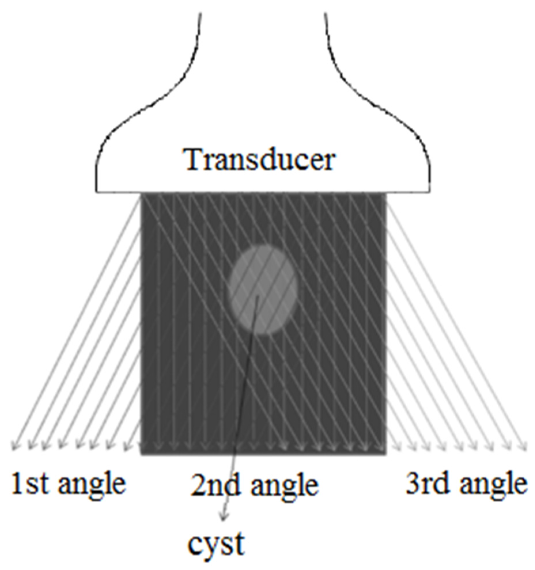
Plane wave firings with different steering angles for coherent plane wave compounding (CPWC). The cyst target is within the overlapped region of all plane waves.
Figure 2.
Plane wave firings with different steering angles for coherent plane wave compounding (CPWC). The cyst target is within the overlapped region of all plane waves.
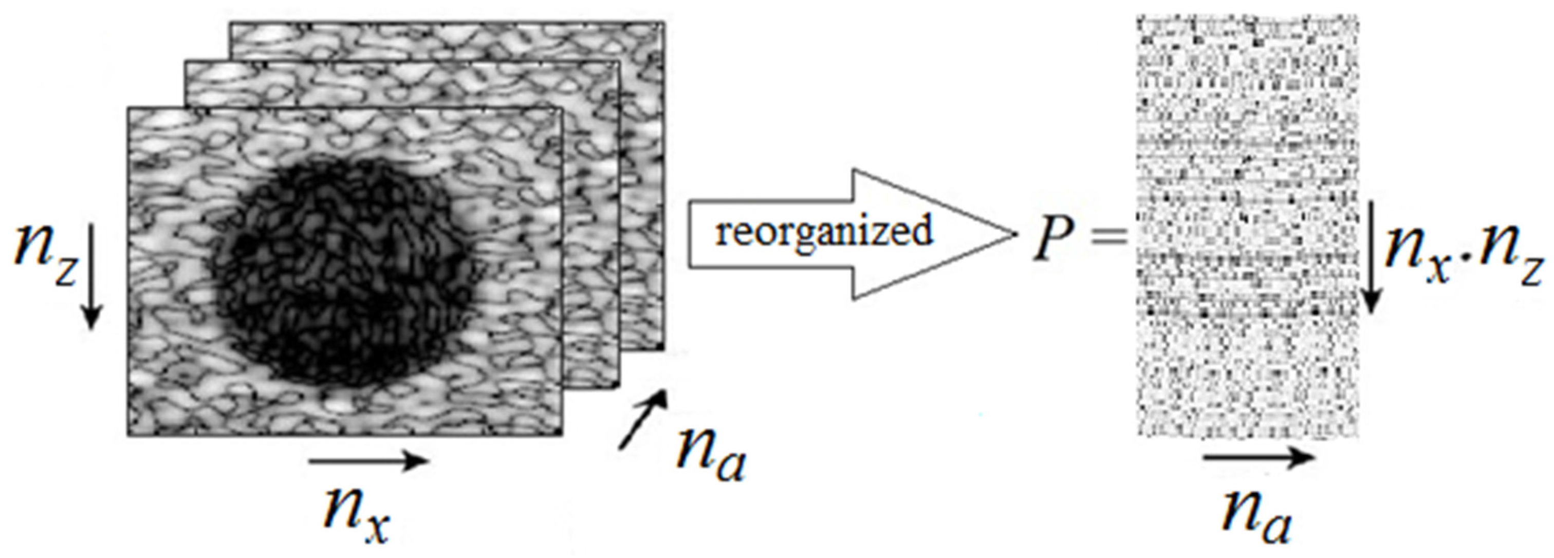
Figure 3.
The CPWC acquisitions form a 3D stack of images with two spatial dimensions (nx, nz) and one angular dimension (na). It is reshaped in a 2D spatio-angular representation (P) where all pixels at one angle are arranged in one column (nx.nz). As a consequence, all angle points for one pixel are arranged in one row (na).
Figure 4.
The graphical explanation of the proposed singular value decomposition (SVD) filter (N represents the rank of matrix P).
Figure 4.
The graphical explanation of the proposed singular value decomposition (SVD) filter (N represents the rank of matrix P).
Figure 5.
The covariance matrix of dimension is presented here.
Figure 5.
The covariance matrix of dimension is presented here.
Figure 6.
Beamformed responses of the simulated point spread function (PSF): (a) CPWC; (b) CPWC with Hamming window; and (c) CPWC + SVD. All images are shown with a dynamic range of 60 dB.
Figure 6.
Beamformed responses of the simulated point spread function (PSF): (a) CPWC; (b) CPWC with Hamming window; and (c) CPWC + SVD. All images are shown with a dynamic range of 60 dB.
Figure 7.
The lateral variation of CPWC, CPWC + Hamming window and CPWC + SVD at the depth of 20 mm.
Figure 7.
The lateral variation of CPWC, CPWC + Hamming window and CPWC + SVD at the depth of 20 mm.
Figure 8.
Beamformed images of simulated cyst phantom: (a) CPWC; (b) CPWC with Hamming window; and (c) CPWC + SVD. All images are shown with a dynamic range of 60 dB.
Figure 8.
Beamformed images of simulated cyst phantom: (a) CPWC; (b) CPWC with Hamming window; and (c) CPWC + SVD. All images are shown with a dynamic range of 60 dB.
Figure 9.
Beamformed images of a point and a hyperechoic region phantom: (a) CPWC; (b) CPWC with Hamming window; and (c) CPWC + SVD. All images are shown with a dynamic range of 60 dB.
Figure 9.
Beamformed images of a point and a hyperechoic region phantom: (a) CPWC; (b) CPWC with Hamming window; and (c) CPWC + SVD. All images are shown with a dynamic range of 60 dB.
Figure 10.
Beamformed images of cyst phantom: (a) CPWC; (b) CPWC with Hamming window; and (c) CPWC + SVD. All images are shown with a dynamic range of 60 dB.
Figure 10.
Beamformed images of cyst phantom: (a) CPWC; (b) CPWC with Hamming window; and (c) CPWC + SVD. All images are shown with a dynamic range of 60 dB.
Figure 11.
Beamformed responses of the simulated PSF: (a) CPWC using five angles; (b) CPWC using 11 angles; (c) CPWC using 21 angles; (d) CPWC + SVD using five angles; (e) CPWC + SVD using 11 angles; and (f) CPWC + SVD using 21 angles. All images are shown with a dynamic range of 60 dB.
Figure 11.
Beamformed responses of the simulated PSF: (a) CPWC using five angles; (b) CPWC using 11 angles; (c) CPWC using 21 angles; (d) CPWC + SVD using five angles; (e) CPWC + SVD using 11 angles; and (f) CPWC + SVD using 21 angles. All images are shown with a dynamic range of 60 dB.
Table 1.
The settings for the computer simulation and phantom experiment.
Table 1.
The settings for the computer simulation and phantom experiment.
| Parameter | Simulation | Phantom Experiment |
|---|
| Pitch | 0.30 mm | 0.30 mm |
| Element width | 0.27 mm | 0.27 mm |
| Element height | 5 mm | 5 mm |
| Elevation focus | 20 mm | 20 mm |
| Number of elements | 128 | 128 |
| Aperture | 38.4 mm | 38.4 mm |
| Transmit frequency | 5.208 MHz | 5.208 MHz |
| Sampling frequency | 20.832 MHz | 20.832 MHz |
| Pulse bandwidth | 67% | 67% |
| Excitation | 2.5 cycles | 2.5 cycles |
| Transmit voltage | - | 30 V |
Table 2.
Full-width at half-maximum (FWHM) and peak sidelobe (PSL) for beamformed responses at z = 20.0 mm.
Table 2.
Full-width at half-maximum (FWHM) and peak sidelobe (PSL) for beamformed responses at z = 20.0 mm.
| Beamformer | FWHM (mm) | PSL (dB) |
|---|
| CPWC | 0.46 | −25.62 |
| CPWC + Hamming | 0.89 | −31.76 |
| CPWC + our SVD filter | 0.46 | −31.80 |
Table 3.
Contrast ratio (CR) and contrast-to-noise ratio (CNR) of the simulated cyst phantom.
Table 3.
Contrast ratio (CR) and contrast-to-noise ratio (CNR) of the simulated cyst phantom.
| Beamformer | CR (dB) | CNR |
|---|
| CPWC | 27.85 | 3.11 |
| CPWC + Hamming | 31.37 | 3.34 |
| CPWC + our SVD filter | 33.52 | 3.48 |
Table 4.
FWHM for the beamformed responses at z = 28.0 mm and the CR and CNRof the hyperechoic cyst.
Table 4.
FWHM for the beamformed responses at z = 28.0 mm and the CR and CNRof the hyperechoic cyst.
| Beamformer | FWHM (mm) | CR (dB) | CNR |
|---|
| CPWC | 0.59 | 18.26 | 2.05 |
| CPWC + Hamming | 0.64 | 20.41 | 2.18 |
| CPWC + our SVD filter | 0.59 | 20.88 | 2.21 |
Table 5.
CR and CNR of anechoic cyst phantom.
Table 5.
CR and CNR of anechoic cyst phantom.
| Beamformer | CR (dB) | CNR |
|---|
| CPWC | 16.72 | 1.89 |
| CPWC + Hamming | 23.49 | 2.36 |
| CPWC + our SVD filter | 23.47 | 2.36 |
Table 6.
The run time (s) of three beamformers in four experiments.
Table 6.
The run time (s) of three beamformers in four experiments.
| Beamformer | PSF | Simulated Cyst | Point Phantom | Cyst Phantom |
|---|
| CPWC | 15.35 s | 3.15 s | 19.74 s | 2.57 s |
| CPWC + Hamming | 15.38 s | 3.16 s | 19.78 s | 2.58 s |
| CPWC + our SVD filter | 15.49 s | 3.28 s | 19.89 s | 2.71 s |
Table 7.
The run time in the PSF simulation using different angle numbers.
Table 7.
The run time in the PSF simulation using different angle numbers.
| Angles | Time for DAS | Time for SVD | Total Time |
|---|
| 5 | 6.98 s | 0.019 s | 7.01 s |
| 11 | 15.34 s | 0.141 s | 15.49 s |
| 21 | 27.89 s | 0.834 s | 28.73 s |
© 2016 by the authors; licensee MDPI, Basel, Switzerland. This article is an open access article distributed under the terms and conditions of the Creative Commons Attribution (CC-BY) license (http://creativecommons.org/licenses/by/4.0/).


