Analysis of the Numerical Diffusion in Anisotropic Mediums: Benchmarks for Magnetic Field Aligned Meshes in Space Propulsion Simulations

Abstract

This manuscript explores numerical errors in highly anisotropic diffusion problems. First, the paper addresses the use of regular structured meshes in numerical solutions versus meshes aligned with the preferential directions of the problem. Numerical diffusion in structured meshes is quantified by solving the classical anisotropic diffusion problem; the analysis is exemplified with the application to a numerical model of conducting fluids under magnetic confinement, where rates of transport in directions parallel and perpendicular to a magnetic field are quite different. Numerical diffusion errors in this problem promote the use of magnetic field aligned meshes (MFAM). The generation of this type of meshes presents some challenges; several meshing strategies are implemented and analyzed in order to provide insight into achieving acceptable mesh regularity. Second, Gradient Reconstruction methods for magnetically aligned meshes are addressed and numerical errors are compared for the structured and magnetically aligned meshes. It is concluded that using the latter provides a more correct and straightforward approach to solving problems where anisotropicity is present, especially, if the anisotropicity level is high or difficult to quantify. The conclusions of the study may be extrapolated to the study of anisotropic flows different from conducting fluids.

1. Introduction

The use of Computational Fluid Dynamics (CFD) is becoming widespread in all branches of engineering due to advances in the development of numerical methods and the increase in achievable computational power. One of the main difficulties to be addressed is the generation of an adequate mesh for the simulated domain, since most numerical errors depend on the mesh quality (see [1]). Due to this reason, one of the most important parts of CFD modeling works found in the literature is the mesh independence analysis [2,3,4]. There are efforts specially devoted to meshing strategies in complex flow simulations [5,6]. Galindo et al. [7] presented an innovative mesh independence analysis that allows to optimize the mesh distribution. The analysis was successfully applied to unstructured meshes in several works [8,9].

The review by Voloshin [10] shows that origin of anisotropy in fluid flows might come from different sources. Several works on the literature deal with flow anisotropy in relativistic flows [11,12] or microfluidic devices [13]. The present work is focused on the anisotropy existing in conducting fluids under the effect of a magnetic field. The study of the motion of conducting fluids has been performed by several authors [14]. The current manuscript is focused in the numerical analysis of the flow behavior of magnetized conducting fluids, such as the plasmas found in electric propulsion devices and, more in particular, related to the electron flow, which is generally the only “magnetized” species, i.e. the plasma is mesomagnetized. Furthermore, since electrons are generally well confined by electric and magnetic fields, a typical assumption in the modeling of the electron population is to consider a quasi-maxwellian fluid of a highly anisotropic nature, in which transport in the perpendicular and parallel directions to the magnetic field is widely different (see [15]).

The classical plasma transport theory states that the perpendicular electron transport coefficient is inversely proportional to the square of the magnetic field strength, $B^{-2}$ and is always smaller, up to various orders of magnitude, than the parallel transport coefficient [15]. This anisotropicity of the transport coefficients may induce a numerical error when numerically solving the flow transport equations, the error becoming more significant if the computational mesh is unaligned with the principal magnetic directions. This numerical error is commonly known as numerical diffusion. Meier et al. [16] analyzed this problem by solving the heat conduction equation with the high-order spectral element code SEL/HiFi [17]. The study concluded that even small grid misalignments cause significant numerical error. The error could be reduced by refining the mesh or by increasing the order of the dicretization elements. A similar study was conducted by Anderson [18] demonstrating that a numerical diffusion arises when solving the Magneto-Hydro-Dynamic (MHD) equations in an axisymmetric 2D Cartesian grid with the magnetic field misaligned with respect to the grid directions. The work showed that even in the limit of anisotropy ratio tending to ∞ (zero perpendicular transport), the flow field showed non-zero perpendicular transport.

As shown in the previously described works, numerical diffusion can be reduced by refining the mesh or increasing the order of the numerical method [16,18]. Another possible mechanism to decrease the influence of this artificial numerical diffusion on the solution is the use of a mesh that is aligned with the the preferential directions of the problem; in the case of conducting fluids, those defined by the magnetic field. Indeed, in the particular case of the electron transport, because of the large anisotropicity in coefficients for the parallel and perpendicular directions, solving the governing equations in a mesh which is misaligned with respect to the magnetic field may lead to cross-contamination of the transport coefficients and thus to numerical diffusion.

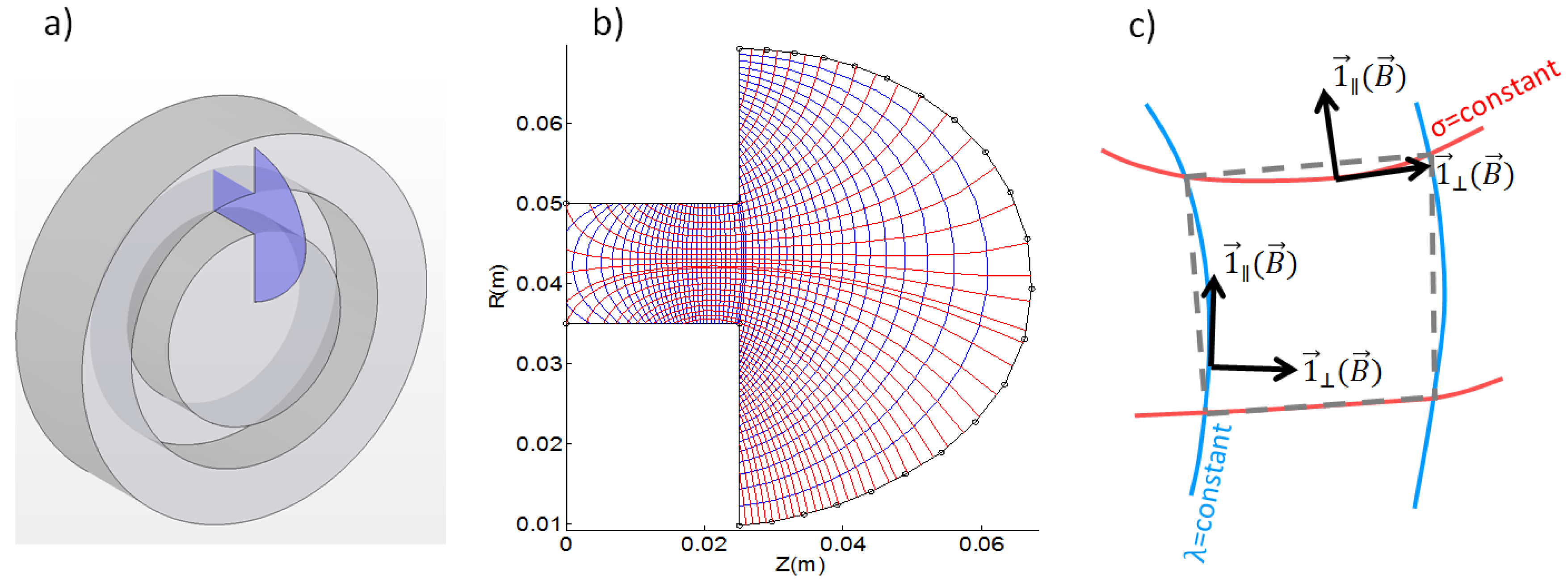
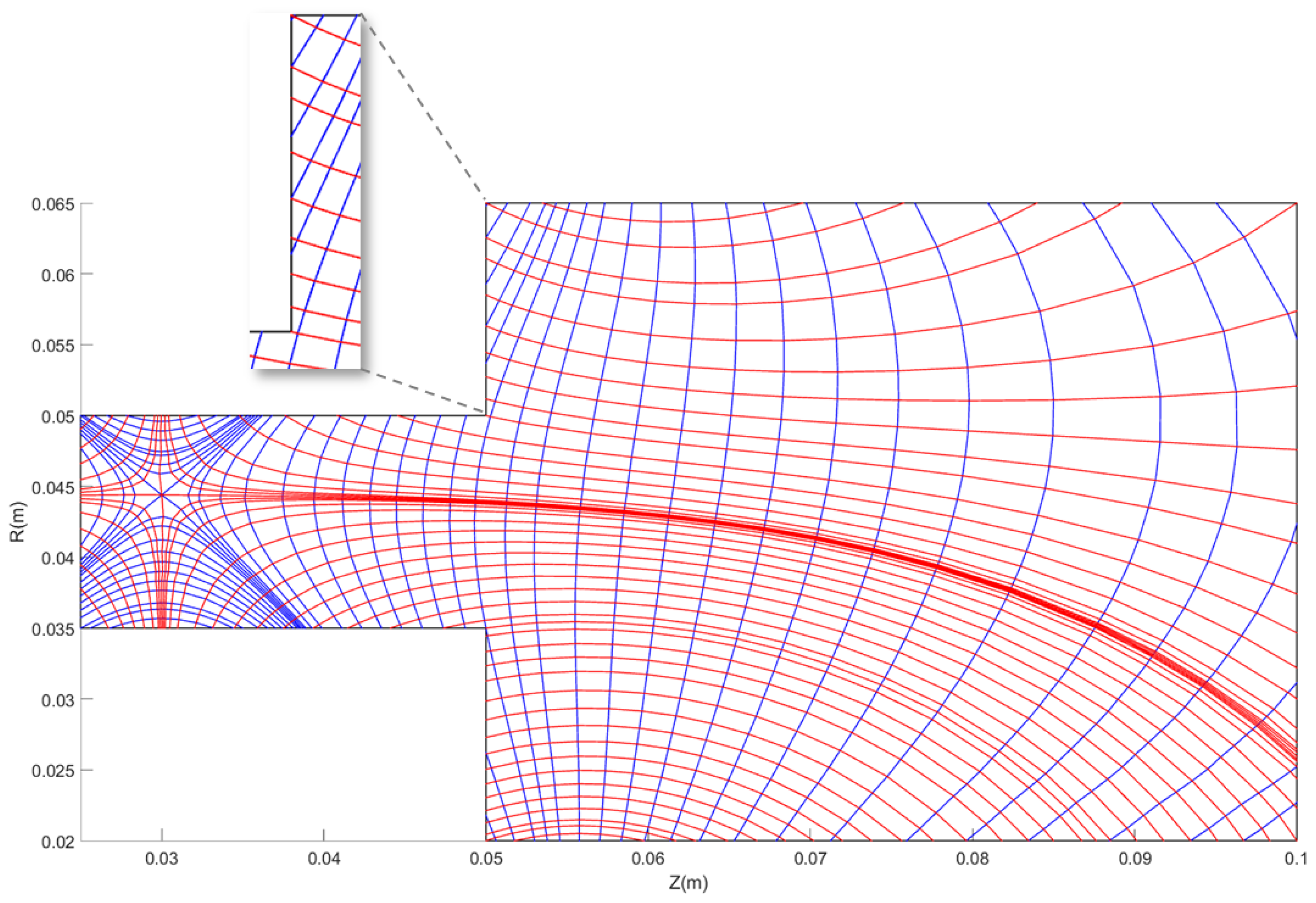
Therefore, for the evolution of the electron population, it seems advisable to solve the governing equations in a curvilinear system of coordinates defined by the local magnetic field directions. This type of mesh is known as Magnetic Field Aligned Mesh (MFAM). In the cases in which this magnetic field may be considered stationary (i.e., the magnetic field $\overrightarrow{B}$ can be assumed irrotational in addition to solenoidal and stationary); the mesh whose element facets are locally aligned with the magnetic field directions is an input to the simulation and does not vary with the plasma flow development. An example of a typical axisymmetric simulation domain of a Hall Effect Thruster (HET) geometry is presented in Figure 1a. Figure 1b shows an example of MFAM and a cell detail is presented in Figure 1c.

The MFAM venue has been utilized extensively both by the plasma fusion [19] and the plasma propulsion [20,21] communities, and numerical diffusion has been documented in simulations for highly anisotropic systems [16,22]. However, a number of difficulties still arise when using the MFAM, mainly in relation to low quality meshes, problematic boundary elements, calculation of gradients and the errors associated with them, as discussed by Araki [23]. These difficulties have increased in modern plasma thruster designs with non-regular magnetic field topologies, which include: Singular points and cusp regions [24].

In the present work, efforts have been carried out to analyze the flow behavior and to justify using the MFAM as opposed to regular, structured, meshes. This analysis has been performed, following the discussion by Araki [23], and tackling the issues of numerical diffusion in regular meshes and comparing it with the solutions obtained in MFAM. Different meshing strategies and problems arising from mesh quality and gradient reconstruction accuracy in magnetically aligned meshes are also addressed. Additionally, a benchmark test is presented showcasing the benefits of using MFAMs versus structured meshes in anisotropic plasmas.

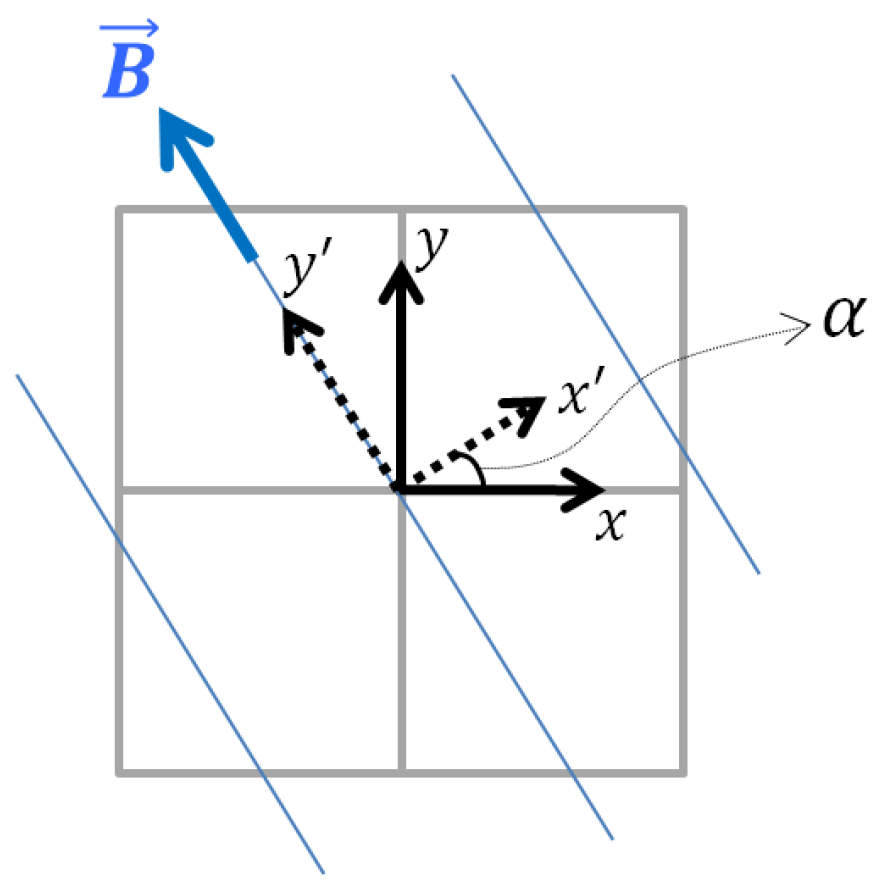
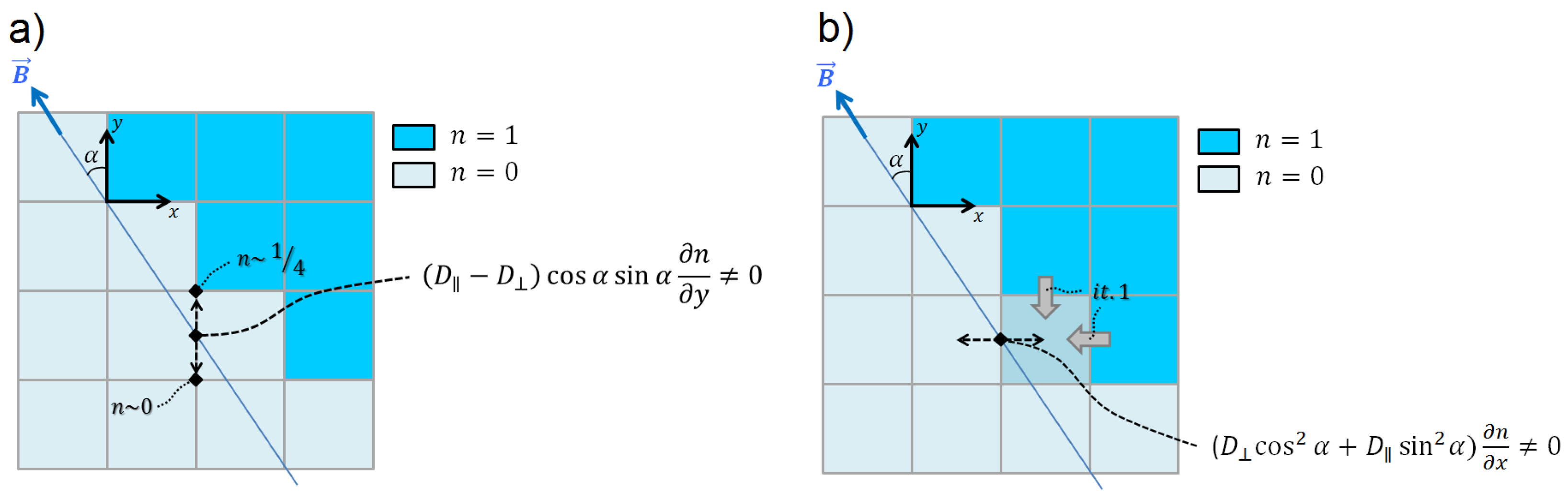
This manuscript is organized as follows: Section 2 explores the issue of numerical diffusion in a regular, structured, mesh for a typical diffusion problem in an anisotropic media. Section 3 is dedicated to meshing strategies for the MFAM and their effects on mesh quality. Section 4 addresses the necessity for gradient reconstruction in an unstructured mesh when solving for the electron fluid equations, proposes the Weighted Least Squares Face Interpolation (WLSQRFI) method as a suitable solution, and computes error estimates for its use. Finally, Section 5 presents benchmark results for the anisotropic diffusion problem in an MFAM versus a regular, structured, mesh and Section 6 concludes the article by reviewing the results presented.

2. Numerical Diffusion in Regular, Structured, Meshes: The Anisotropic Diffusion Problem

The classical anisotropic diffusion problem in magnetized fluids is well known: It is similar to the ambipolar diffusion problem (in which an ambipolar electric field is established to balance the fluxes of the electron and ion species), except that the parallel ($\parallel$) and perpendicular (⊥) transport coefficients account for the anisotropy of the problem.

2.1. Problem Formulation

The mathematical model describing the flow motion as derived by Simon [25], considering plasma quasineutrality $n_e\approx n_i=n$, for an infinite 2D slab with conducting walls under a straight magnetic field can be expressed as

$$\begin{array}{c}\hfill \frac{dn}{dt}=\left[\begin{array}{cc}\frac{{\mu }_{e\parallel }{D}_{i\perp }-{\mu }_{i\parallel }{D}_{e\perp }}{{\mu }_{e\parallel }-{\mu }_{i\parallel }}& 0\\ 0& \frac{{\mu }_{e\parallel }{D}_{i\parallel }-{\mu }_{i\parallel }{D}_{e\parallel }}{{\mu }_{e\parallel }-{\mu }_{i\parallel }}\end{array}\right]\left[\begin{array}{c}\frac{{\partial }^{2}n}{\partial x^{\prime 2}}\\ \frac{{\partial }^{2}n}{\partial y^{\prime 2}}\end{array}\right],\end{array}$$

(1)

where n is the fluid density, the μ terms are the mobility coefficients for both species, and $D_{\perp }$ and $D_{\parallel }$ are, respectively, the diffusion coefficients across the magnetic field and the “free” or natural diffusion coefficient. The former coefficient accounts for classical collision mechanisms, while the latter one appears in the non-confining direction parallel to the magnetic field.The variables $x^{\prime }$ and $y^{\prime }$ are, respectively, the coordinates associated to the directions perpendicular (${\overrightarrow{1}}_{\perp }$) and parallel (${\overrightarrow{1}}_{\parallel }$) to the magnetic field as shown in Figure 1.

For the sake of simplicity, the effects of the ambipolar perpendicular electric field for non-conducting walls can be neglected and the diffusion term can be considered uniform across the flow domain. Under these assumptions, the diffusion terms can be written as:

$$\begin{array}{c}\hfill \begin{array}{c}{\mathcal{D}}^{\prime }=\left[\begin{array}{cc}{D}_{\perp }& 0\\ 0& D_{\parallel }\end{array}\right]\end{array}.\end{array}$$

(2)

Then, the diffusion coefficient ratio can be defined as $\mathrm{\Theta }=\frac{D_{\parallel }}{D_{\perp }}$ and it is the main parameter in this study, as it determines the rate of numerical diffusion. Formally, the flow behavior can be modeled as the classical diffusion equation (Equation (1)), taking into account the flux vector Γ and strictly positive diffusion coefficients as

$$\begin{array}{c}\hfill \frac{dn}{dt}={\nabla }^{\prime }\times \left[{\mathcal{D}}^{\prime }\times {\nabla }^{\prime }n\right]={\nabla }^{\prime }\times \overrightarrow{{\mathrm{\Gamma }}^{\prime }}={\nabla }^{\prime }\times \left[\begin{array}{c}{\mathrm{\Gamma }}_{x^{\prime }}\\ {\mathrm{\Gamma }}_{y^{\prime }}\end{array}\right]\end{array}$$

(3)

The numerical diffusion problem arises when the diffusion equation (Equation (3)) is discretized in a coordinate system which is not aligned with the perpendicular and parallel directions of the magnetic field, such as a Cartesian coordinate system for a randomly aligned magnetic field as represented in Figure 2. For the sake of simplicity, let’s consider that magnetic field lines are straight (but the problem is easily generalizable to a curved field) and magnetic versors (${\overrightarrow{1}}_{\perp }$, ${\overrightarrow{1}}_{\parallel }$ defined in Figure 1) are rotated a given angle α with respect to the Cartesian system as shown in Figure 2.

The rotation matrix $\mathcal{R}$ allows for transforming Equation (3) into the Cartesian coordinate frame by using the relations:

$$\begin{array}{ccc}\hfill \mathcal{R}& =\hfill & \left[\begin{array}{cc}cos\alpha & -sin\alpha \\ sin\alpha & cos\alpha \end{array}\right];\hfill \\ \hfill \overrightarrow{\mathrm{\Gamma }}& =\hfill & \mathcal{R}\times \overrightarrow{{\mathrm{\Gamma }}^{\prime }};\hfill \\ \hfill {\nabla }^{\prime }n& =\hfill & \mathcal{R}\times \nabla n.\hfill \end{array}$$

(4)

Replacing in Equation (3), results in the diffusion equation in Cartesian coordinates which satisfies:

$$\frac{dn}{dt}=\nabla \times \left[{\mathcal{R}}^{-1}{\mathcal{D}}^{\prime }\mathcal{R}\times \nabla n\right];$$

(5)

with the new diffusion matrix $\mathcal{D}$ being:

$$\begin{array}{c}\mathcal{D}={\mathcal{R}}^{-1}{\mathcal{D}}^{\prime }\mathcal{R}=\left[\begin{array}{cc}{D}_{\perp }{cos}^2\alpha +D_{\parallel }{sin}^2\alpha & \left(D_{\parallel }-D_{\perp }\right)cos\alpha sin\alpha \\ \left(D_{\parallel }-D_{\perp }\right)cos\alpha sin\alpha & D_{\parallel }{cos}^2\alpha +D_{\perp }{sin}^2\alpha \end{array}\right].\end{array}$$

Integrating Equation (5) over each mesh volume and applying the Gauss divergence theorem, the following relationship is obtained:

$$\begin{array}{c}\hfill \underset{V}{\int }\frac{dn}{dt}=\underset{A}{\oint }\left[\begin{array}{c}(D_{\perp }{cos}^2\alpha +D_{\parallel }{sin}^2\alpha )\frac{\partial n}{\partial x}+\left(\left(D_{\parallel }-D_{\perp }\right)cos\alpha sin\alpha \frac{\partial n}{\partial y}\right)\\ \left(\left(D_{\parallel }-D_{\perp }\right)cos\alpha sin\alpha \frac{\partial n}{\partial x}\right)+(D_{\parallel }{cos}^2\alpha +D_{\perp }{sin}^2\alpha )\frac{\partial n}{\partial y}\end{array}\right]\times d\overrightarrow{A}.\end{array}$$

(6)

Equation (6) must be satisfied for every mesh element and is analogous to the one derived by Wirz [26]. Equation (6) illustrates how numerical diffusion appears in non-aligned meshes. Indeed, the diffusion term expressed in Cartesian coordinates will be responsible for the aforementioned cross-contamination, when $D_{\parallel }\gg D_{\perp }$. Numerical diffusion appears even when the plasma is perfectly confined, i.e., the diffusion coefficient ratio is $\mathrm{\Theta }\to \infty$ (or $D_{\perp }=0$). This may be simply understood through the sketch in Figure 3. First, the cross-diffusion term induces a transfer of mass between contiguous cells when none should occur (Figure 3a); second, for $\mathrm{\Theta }\to \infty$ magnetic field lines are impermeable to mass-flow, and yet, because of the iterative nature of numerical solutions, mass will be transported through the mesh cells (Figure 3b) due to the lack of alignment between the mesh and the magnetic field.

2.2. Case results

In the present work, Equation (6) is solved by applying the Finite Volume Method (FVM, see [1] for further reference). The selection of this method is done since it provides a formulation of the problem in conservative form (versus the weak forms of the Finite Element and Finite Differences Methods). For a particular mesh volume element, the former equation is discretized by an explicit Euler method as:

$$\begin{array}{c}\begin{array}{c}{V}_i\frac{n_{e,i}^{t+\Delta t}-n_{e,i}^t}{\Delta t}=\\ ={\displaystyle \sum _j}\left({\left.\left[\begin{array}{c}(D_{\perp }{cos}^2\alpha +D_{\parallel }{sin}^2\alpha )\frac{\partial n}{\partial x}+\left(\left(D_{\parallel }-D_{\perp }\right)cos\alpha sin\alpha \frac{\partial n}{\partial y}\right)\\ \left(\left(D_{\parallel }-D_{\perp }\right)cos\alpha sin\alpha \frac{\partial n}{\partial x}\right)+(D_{\parallel }{cos}^2\alpha +D_{\perp }{sin}^2\alpha )\frac{\partial n}{\partial y}\end{array}\right]\right|}_{f,j}\times d{A}_{f,j}{\overrightarrow{n}}_{f,j}\right),\end{array}\end{array}$$

(7)

where the subscript“$e,i$” represents the $i^{th}$ element and “$f,j$” the $j^{th}$ facet of that element. Derivatives on the regular structured mesh are approximated by a central differences scheme, as:

$$\begin{array}{ccc}\hfill \frac{\partial n}{\partial x}& \approx \hfill & \frac{n_2-n_1}{\Delta x}\hfill \\ \hfill \frac{\partial n}{\partial y}& \approx \hfill & \frac{1}{\Delta y}\times \left(\frac{n_1+n_2+n_3+n_4}{4}-\frac{n_1+n_2+n_5+n_6}{4}\right)\hfill \end{array}$$

(8)

where the $n_i$ terms are the ones illustrated in Figure 4. Equation (8) is applied to each volume element of the domain leading to a system of algebraic equations, which can be written as: $\left[A\right]\left\{n\right\}=\left\{B\right\}$. Where $\left\{n\right\}$ are the unknowns of the problem and $\left[A\right]$ is a sparse matrix. The system is solved numerically to obtain the temporal evolution of the anisotropic diffusion problem (for a given value of $\mathrm{\Theta }=D_{\parallel }/D_{\perp }$) for the limit case of non-permeable walls under a magnetic field forming an angle α with the Cartesian system. The system evolution for $\alpha =-{45}^{\circ }$ and $\mathrm{\Theta }\to \infty$ is presented in Figure 5, illustrating the appearance of numerical diffusion, since the red line represents a magnetic field line and as such should be impermeable to the plasma.

The errors due to numerical diffusion could be quantified computing the average error density for the elements in the low density zone (at the left side of the red line in Figure 5). The ideal behavior will be to consider that the plasma should be perfectly confined, as it is set in the initial condition, that is:

$$〈error(t)〉=\frac{1}{N_{elem}}\sum _{i=1}^N\frac{\left|n_i(t)-n(t=0)\right|}{n(t=0)}.$$

(9)

Figure 6 shows the evolution of the error due to numerical diffusion for the $\mathrm{\Theta }\to \infty$ case, with different values of α, and different number of mesh elements. Figure 6a shows that the error increases with time and Figure 6b shows how this error is reduced when increasing the number of cells in the computational domain.

Another interesting analysis corresponds to the concept of effective diffusion coefficient ratio, ${\mathrm{\Theta }}_{eff}$. This coefficient provides an equivalent diffusive mass flux in a problem in which the mesh and magnetic fields are aligned, for a given simulation domain, mesh resolution, initial condition, and the parameters α and Θ.

Table 1. Effective diffusion coefficient ratio (${\mathrm{\Theta }}_{eff}$) for different mesh resolutions, alignment of the magnetic field (α) and diffusion coefficient ratios (Θ).

Mesh resolution	${\mathbf{\Theta }}_{\mathbf{eff}}\sim ...$	$\mathbf{\Theta }\to \mathbf{\infty }$	$\mathbf{\Theta }=100$	$\mathbf{\Theta }=10$
50 elements	$\alpha ={20}^{\circ }$	∼5	∼4	∼3
	$\alpha ={45}^{\circ }$	∼5	∼5	∼3
	$\alpha ={60}^{\circ }$	∼5	∼5	∼3
500 elements	$\alpha ={20}^{\circ }$	∼20	∼15	∼5
	$\alpha ={45}^{\circ }$	∼25	∼15	∼5
	$\alpha ={60}^{\circ }$	∼20	∼15	∼6
5000 elements	$\alpha ={20}^{\circ }$	∼50	∼25	∼8
	$\alpha ={45}^{\circ }$	∼50	∼30	∼8
	$\alpha ={60}^{\circ }$	∼50	∼30	∼7

presents results for the effective diffusion coefficient for different parameter sets (Θ, α, and number of cells) for the problem described by Equation (6). The problem is solved through the explicit Euler/FVM discretization of Equation (7).

Results are in agreement with those from the literature [16,18]. Numerical diffusion leads to a reduction in the anisotropicity of the system, as accounted by the effective Θ. For the explored sets, the errors are just slightly dependent on the misalignment of the magnetic field and the mesh, α, when the mesh resolution is sufficiently fine. Errors are however very noticeable for lower resolution meshes and the accuracy is only partially improved through refinement for the high anisotropicity cases.

3. Meshing Strategies for Curvilinear Meshes Aligned with the Preferential Directions of the Problem

The analysis presented in the previous section concludes that numerical diffusion is an important issue in numerical simulations of highly anisotropic flow, and therefore some steps should be taken to avoid it. One of the possible solutions is the use of meshes aligned with preferential directions of the problem, as defined by the cause of the anisotropy. In the case of conducting fluids, this cause is the magnetic field, and thus the use of a Magnetic Field Aligned Mesh (MFAM) is proposed.

A stationary MFAM can be built when the magnetic field in the simulated domain can be considered to be both irrotational, $\nabla \times \overrightarrow{B}\approx 0$, solenoidal, $\nabla \times \overrightarrow{B}=0$, and stationary, $\frac{\partial \overrightarrow{B}}{\partial t}=0$. The irrotational approximation is valid whenever the effect of the flow discharge over the external magnetic field is small compared to the field generated by the magnetic circuit. If these conditions are not fulfilled, then the magnetic field will be dependent on the flow motion and thus the mesh will not be constant during the simulation.

In a typical axisymmetric simulation domain (Figure 1) and in 2D planar one, the above magnetic field equations allow one to derive the differential relations below for the magnetic stream-line function λ and the magnetic potential function σ, which can be integrated and become the variables of a curvilinear system of magnetic coordinates.

$$\nabla \times \overrightarrow{B}=0\to {\nabla }^2\lambda =0\to \frac{\partial \lambda }{\partial r}=-r{B}_z;\frac{\partial \lambda }{\partial z}=r{B}_r$$

(10)

$$\nabla \times \overrightarrow{B}\approx 0\to \nabla \sigma =\overrightarrow{B}\to \frac{\partial \sigma }{\partial r}=B_r;\frac{\partial \sigma }{\partial z}=B_z$$

(11)

Lines of constant λ always follow the local direction of the magnetic field (${\overrightarrow{1}}_{\parallel }$) and lines of constant σ are always in the perpendicular direction to the magnetic field (${\overrightarrow{1}}_{\perp }$) as shown in Figure 1a. The intersections of these isolines define the points that are the vertexes of the volumes of the constructed mesh. Theoretically, the solution for a highly anisotropic problem posed in the magnetic reference frame should minimize the numerical diffusion caused by anisotropicity, although some numerical errors will remain; those due to discretization and the flatness of MFAM elements, thus losing the information about the local curvature of the magnetic field on the face, as may be seen in Figure 1a. Moreover, building a robust magnetically-aligned mesh in which to solve accurately the flow presents a number of challenges which need to be assessed through different strategies in the meshing algorithm.

Specifically, issues arise regarding mesh quality, mainly at the domain boundaries. Araki et al., [23] tackle these by sacrificing the MFAM configuration in the boundary elements (and in the elements adjacent to them), choosing to relocate node positions to improve quality. His conclusion is that poor mesh quality in the MFAM boundaries leads to errors in the numerical solution which are, at least, comparable to numerical diffusion. The full discussion on this topic is performed for Section 5. Focusing on improvement of mesh quality, correct handling of gradient reconstruction and the implementation of a conservative method, such as the FVM, present other benefits that recommend the use of the MFAM across the domain and diminish the issue of numerical diffusion with little error specific to the non-Cartesian mesh. In the following subsections, the main meshing algorithms are described, followed by the initialization of the process, and finally the capability of manually modifying the mesh surfaces.

3.1. Meshing Algorithms

A Mesh Generator has been specifically built to tackle the generation of Magnetic Field Aligned Meshes. The tasks performed by the Mesh Generator are as follows. First, the magnetic field in the selected simulation domain is obtained. Then, the magnetic variables λ and σ are obtained by integrating over an initial structured Cartesian auxiliary mesh. Once the values of the magnetic variables are computed, the Generator selects a number (chosen by the user) of iso-levels (contour levels). Finally the MFAM mesh information is stored by elements, facets, nodes, etc.

Two main concerns arise when building the MFAM. First, as the magnetic field is not constant in the domain, picking the contour levels of λ and σ to ensure that lines are properly spaced requires careful consideration. This is specially true whenever singular points ($\left|\overrightarrow{B}\right|=0$) or local minima appear in the domain. At those points, because of low magnetic field strength, the variation of λ and σ around these regions is smaller than in regions of high magnetic field strength leading to large elements. The solutions proposed in this work is to add dedicated contour levels in order to avoid excessively large mesh elements. Second, the mesh is determined by the topology of the magnetic field, with the user only being able to adjust the number and which contour levels are picked. This implies that there is little control over the points of intersection of the isolines, and in particular in the intersection of the isolines with the domain contours. This may lead to low quality boundary elements if it is not carefully treated.

3.2. Contour Level Initial Selection

The procedure starts by selecting the number of contour levels, i.e., the number of λ and σ lines, which will populate the simulation domain. The Mesh Generator then uses one of various algorithms in order to generate correctly spaced isolines in the mesh (picking specific contour level values). These algorithms allow the user to explore the best meshing methodology for the particular problem at hand. There are several algorithms or spacing methods in the literature, the ones used in the present work and their main characteristics are described below:

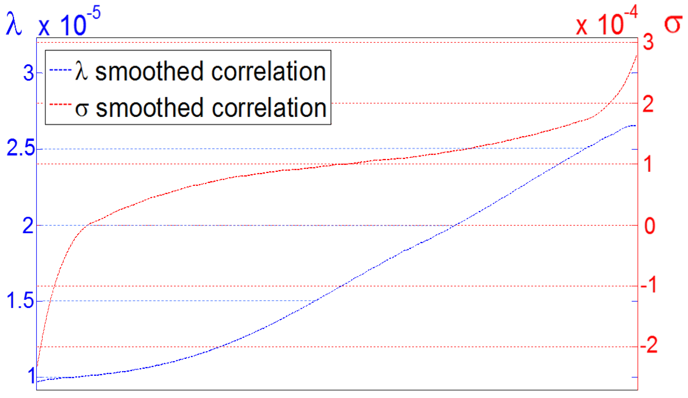
• Smoothing: The values for λ and σ are sorted and smoothed using a local regression method which applies weighted least squares and 2nd degree polynomial models. In this way a correlation between the magnetic coordinate value and the amount of instances it appears in the domain is obtained. Then, the contours levels selected by the user are evenly distributed over the correlation. This procedure is aimed toward obtaining contour level values with a good spatial distribution, regardless of the local rate of variation of the magnetic coordinate, as shown in Figure 7.
• Logarithmic: It obtains logarithmically spaced values for the magnetic coordinate between the maximum and minimum values resulting from the integration. This procedure biases the selection of contour levels toward smaller values (associated with regions of lower magnetic field intensity), avoiding incorrect spacing around high magnetic field intensity regions.
• Exponential-stretching: This method was proposed by Araki et al., [23] as a way to deal with magnetic field topologies containing singular regions and/or high ratios of maximum to minimum field strength. For either of the magnetic coordinates (characterized here as ψ), the number of contour levels, $n_{\psi }$, are obtained from:

  $$\begin{array}{c}\hfill \left\{\begin{array}{c}\begin{array}{c}{\psi }_q={\psi }_{min}\frac{exp\left(\frac{q_0-q}{q_0-1}{\alpha }_{\psi }\right)-1}{exp\left({\alpha }_{\psi }\right)-1}\mathrm{for}q<q_0\\ {\psi }_q={\psi }_{max}\frac{exp\left(\frac{q-q_0}{n_{\psi }-q_0}{\alpha }_{\psi }\right)-1}{exp\left({\alpha }_{\psi }\right)-1}\mathrm{for}q>q_0\end{array}\hfill \end{array}\right.\end{array}$$

  (12)

  where $q_0$ is defined as:

  $$q_0=\int \left(n_{\psi }\frac{{\psi }_{min}}{{\psi }_{max}-{\psi }_{min}}\right)\mathrm{and}\psi (q_0)=0.$$

  (13)

  Equation (12) implies obtaining the contour levels by exponentially stretching from 0 to the maximum positive and negative values of each magnetic coordinate. The parameter ${\alpha }_{\psi }$ is the stretching parameter, and is specified as an input.
• Expanded-exponential-stretching: It is based on the previous method but with an expanded functionality to account for the possibility of having multiple singular points: The algorithm searches the simulation domain for local minima of the magnetic field intensity and identifies the magnetic coordinates, λ and σ that define them. It then allows for specific control of the stretching method around these points, including adding fractional levels for fine tuning of the mesh elements and incorporating the contour lines crossing the singular points, as may be seen in Figure 8. The incorporation of these lines contributes to the avoiding undesired large elements in the singular region. This method has been developed during the present work.

Examples of the meshing algorithms for a typical Hall Effect Thruster magnetic field are shown in Figure 9. The Expanded-exponential-stretching is found to be consistently more robust in achieving meshes where the isolines are evenly distributed through the domain for the different magnetic topologies put to trial.

Figure 8 shows a mesh with a singular point produced using the Expanded-exponential-stretching method. This mesh is typical of some magnetic topologies of modern Hall Effect Thrusters, which try to control better the flow in the upstream region of the thruster channel. Figure 8 shows that this method allows the user a good level of control around the singular point region. At the moment, this is done at the expense of other regions in the domain presenting small and elongated size elements, which could be inadequate computationally. A possible way of addressing this issue in future versions of the algorithm could be through the inclusion of hanging-nodes and clustering of elements [27,28].

3.3. Contour Level Manual Correction

Once initial selection of λ and σ isolines is performed, the obtained mesh will present issues with regards to spacing and boundary elements. In case of the latter, issues arise from: Elements with a variable number of facets (three, four, or five), in comparison to interior elements which are generally four-sided; the appearance of some small area elements, elements with large aspect ratios (where the boundary facet is very small compared to the others), among others. These issues can be seen in the detail of some cells close to the boundary in Figure 8.

In order to improve the quality of the MFAM, and also to provide a tool for fine tuning of the mesh, a functionality has been implemented allowing to manually correct λ and σ isolines via a Graphical User Interface. This fine tuning tool is mainly used close to the domain’s corners, to correct the position of the lines there.

4. Mesh Regularity: Geometric Quality and Gradient Reconstruction in MFAMs

Recent studies on the effects of mesh regularity on the numerical solution, such as the one performed by Diskin [29], indicate that the quality of the mesh cannot be truly assessed without taking into account the nature of the problem, the numerical discretization approach, and the expected computational output, in addition to purely geometric quality indicators. Particularly, the FVM method is referred to by Diskin [29] as being resilient against the effects of non-regularity in non-structured meshes, which provides a good argument favoring its utilization in conjunction with the MFAM approach.

In the following subsection an assessment of the MFAM quality, both geometric and gradient based, without delving into their effects over a particular problem is presented. The idea of this assessment is that, however resilient, errors in terms of discretization, interpolation and gradient calculation (which can be linked both to geometric properties of the mesh and to the methods used for gradient reconstruction) may plague our solution. The conclusion is that it is best to minimize these issues from the start.

4.1. Geometric Mesh Quality

The different possibilities offered by the previously described meshing algorithms and the fine tuning through manual corrections allow the user to iterate through MFAMs with increasingly better geometric quality properties. Nevertheless, high quality meshes will always be difficult to achieve due to the restriction of using isolines which are defined by the magnetic topology over arbitrary simulation domains, and thus requiring special attention to issues appearing close to the domain boundaries.

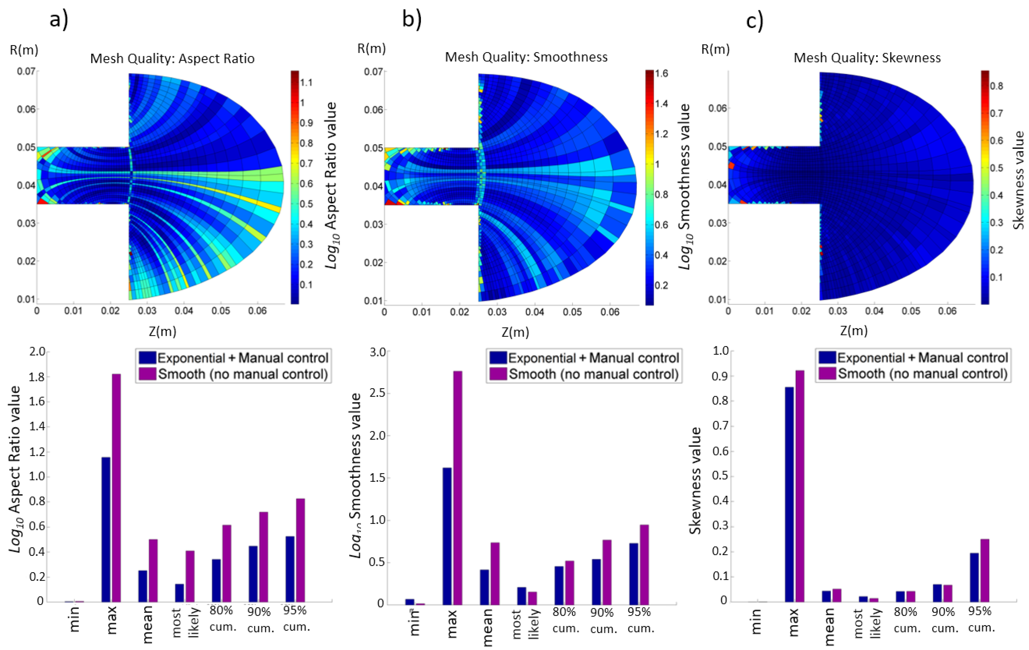
Mesh geometric quality is described through the following set of element properties:

$$\begin{array}{c}\hfill \begin{array}{c}smoothness=\frac{max(A_{element},A_{adjacents})}{min(A_{element},A_{adjacent})}\\ aspectratio=\frac{max(facet-lengt{h}_{element})}{min(facet-lengt{h}_{element})}\\ skewness=max\left[\frac{{\theta }_{max}-{\theta }_e}{{180}^{\circ }-{\theta }_e},\frac{{\theta }_e-{\theta }_{max}}{{\theta }_e}\right]\end{array}\end{array}$$

(14)

where A represents the areas, $element$ and $adjacent$ represent, respectively, the element being considered and the elements adjacent to it, ${\theta }_{max}$ is the largest angle in the element polygon and ${\theta }_e$ is the angle in an equiangular polygon with the same number of sides as the element considered. Large aspect ratios and smoothness may be intuitively understood to affect the interpolation of the solution and gradient reconstruction in the element faces (although this may be offset in part by using a weighted Least Squares (LSQR) method, see Section 4.2); skewness may be related to large errors for fluxes in facets which are nearly parallel and affect the cells in the boundary of the domain.

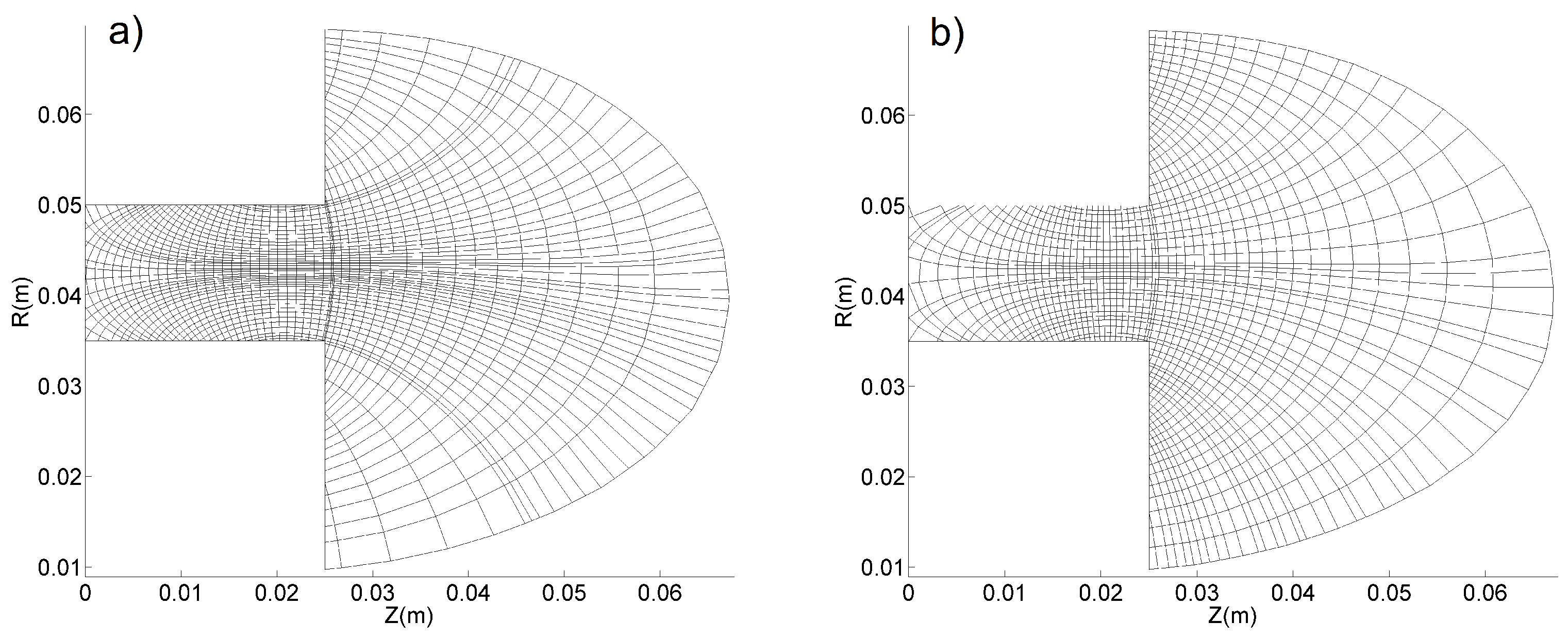
In order to show how the functionality in the Mesh Generator allows one to improve the geometric quality of the MFAM, two different meshes are compared through their quality statistics: One generated using the smoothing method with no manual correction and one generated using the expanded-exponential-stretching method and then applying a manual correction of the mesh. The two meshes used are the ones presented in Figure 9. Figure 10 shows that better geometric quality properties are achieved through the implemented functionality. This better quality is shown by the decrease of the mean, maximum and accumulated values of the different parameters analyzed.

4.2. Gradient Reconstruction

Gradient reconstruction (GR) is required in cell-centered (“element-centered”) FVM schemes in order to obtain partial derivatives of the different flow variables at the element facets. These variables will appear in the discretized equation from the application of the Gauss theorem to the divergence terms in the conservative equation. For structured Cartesian meshes, such as the one employed in Section 2.2, central or upwind differencing schemes retain an acceptable order of accuracy; however, whenever dealing with non-structured meshes, such as the MFAM, higher order differencing schemes become necessary.

Both Diskin [29] and Sozer [30] review the use of the Green-Gauss (GG) and the LSQR (both Weighted -WLSQR- and Unweighted -ULSQR-) methods in terms of order of accuracy for GR; Sozer also performs analysis on additional methods, showcasing that, while consistency in the GG and LSQR methods might vary with mesh regularity, other methods tend to have lower orders of accuracy. Recently several authors have developed hybrid Green–Gauss/Weighted-Least-Squares methods [30,31], which might offer the best compromise between GR methods. However, for the sake of simplicity and since the objective here is to provide an insight to the issues arising in the GR due to low mesh quality, the following analysis is performed using a WLSQR method.

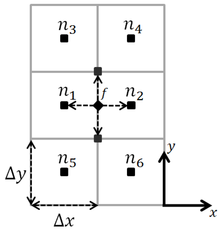
In particular, a method equivalent to the WLSQR Face Interpolation -WLSQRFI- method described by Sozer [30] has been implemented because of the selection of a cell-centered FVM discretization, that requires gradients at the element facets. The method is based on the Taylor series expansion. The resulting set of equations determine the value of any variable ϕ at the facet center, as well as derivatives and cross-derivatives, from the value of ϕ at a chosen number of stencil points (the number will depend on the order of the method) and the set of weights assigned to them. Stencil points are chosen as the centers of the surrounding elements and weights are typically functions of the inverse distance, element areas, and other geometrical parameters. Note that if the weights are chosen to be equal to 1 the method applied is equivalent to the ULSQR. The WLSQR method offers a high level of flexibility to tune the quality of GR in a particular mesh: Since there is freedom for selecting the appropriate weights and order of the Taylor expansion. This can be done independently for interior and boundary elements in the MFAM.

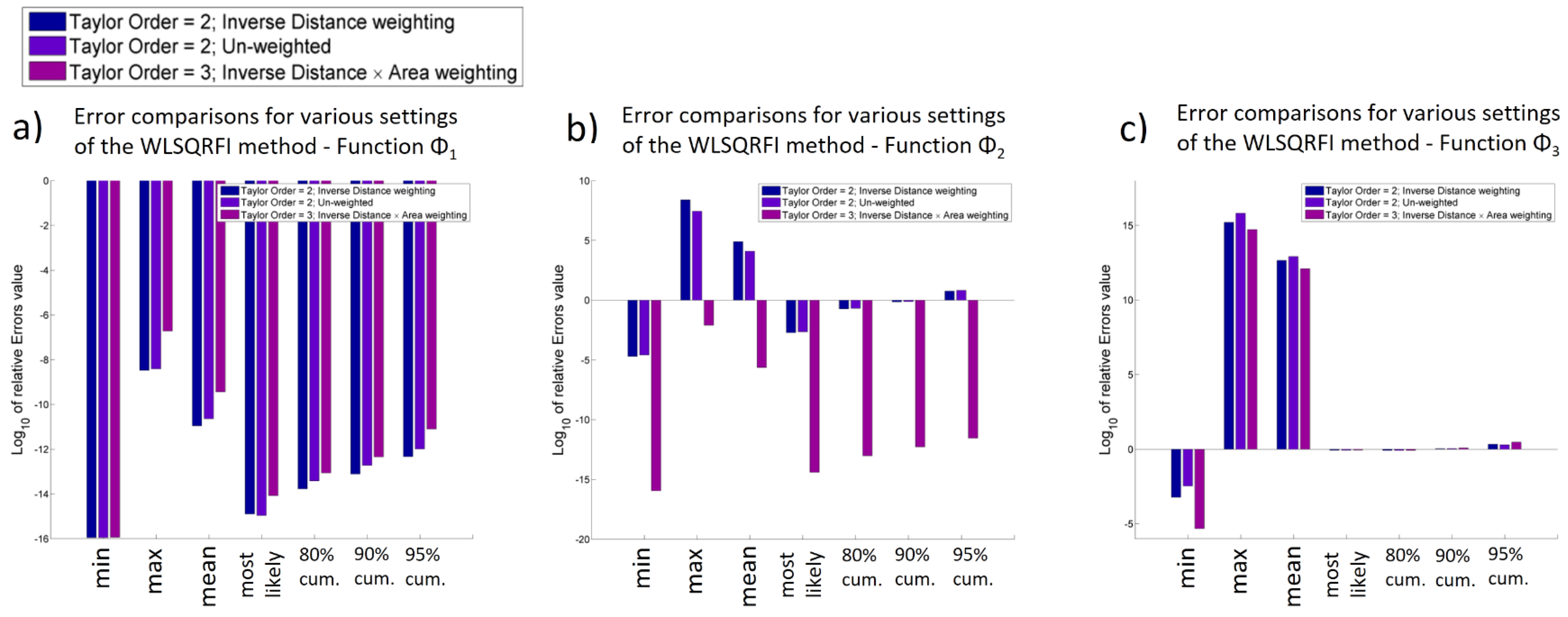
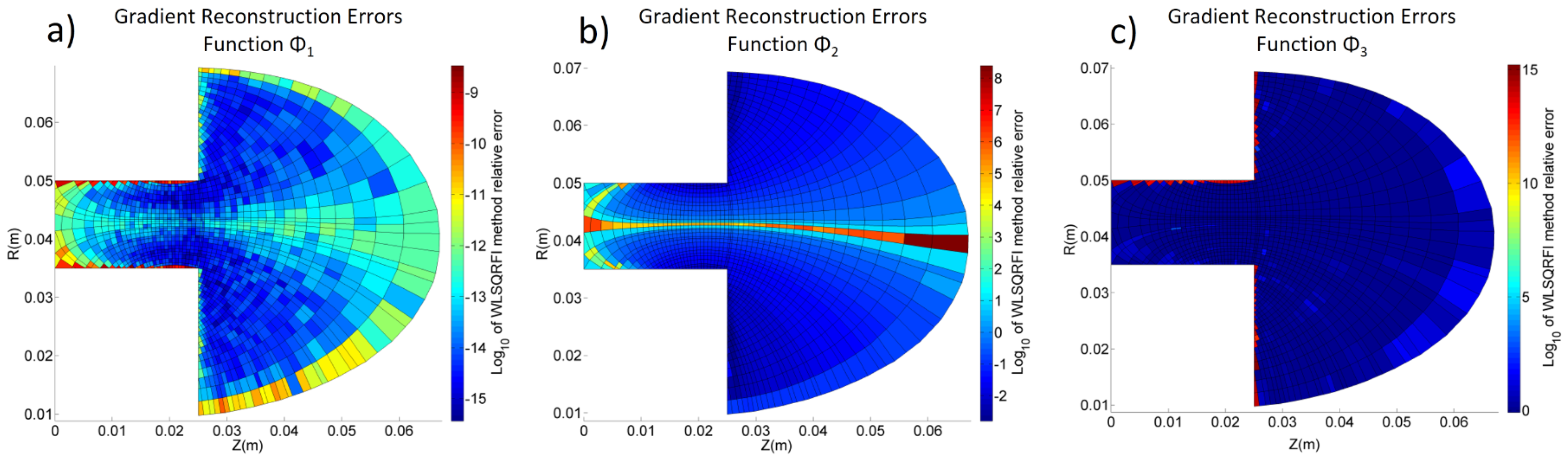
The following analysis shows that the selection of the parameters conferring the flexibility to the method affects greatly the accuracy achieved during the GR. Figure 11 shows errors committed by numerical GR, using inverse-distance weighting for 2nd order development and using 9 stencil points. The method has been applied to the extended-exponential-stretching mesh of Figure 9b and for the following trial functions, ${\varphi }_i\left(\lambda ,\sigma \right)$:

$$\begin{array}{cc}{\varphi }_1\sim & {\lambda }^2+{\sigma }^2\hfill \end{array}$$

(15)

$$\begin{array}{cc}{\varphi }_2\sim & {\lambda }^3\times {\sigma }^3\hfill \end{array}$$

(16)

$$\begin{array}{cc}{\varphi }_3\sim & sin\lambda \times cos\sigma \hfill \end{array}$$

(17)

where λ and σ are the previously defined magnetic coordinates.

Figure 11 shows a certain correlation between low geometric quality regions and large errors in gradient reconstruction, specifically in boundary elements (poor skewness and smoothness) and poor aspect ratio elements. Figure 12 shows variation in error statistics for different weights and Taylor expansion orders for the different trial functions.

In terms of the LSQR method, two aspects become clear: First, selection of the parameters sets the difference between unacceptable and acceptable errors in the calculation of gradients, as inferred from the results from Figure 12b. Second, there are some restrictions in the function that the GR method is able to reconstruct, as shown in Figure 12c: The function ${\varphi }_3$ presents relative errors larger than 1 because the mesh does not provide enough resolution for the LSQR method to correctly obtain the function gradients. This limitation is related to the particular wavelength of the function, and it is not a specific problem of using non-Cartesian meshes, since a similar one will arise in a regular structured mesh with low resolution.

In view of the previous results, it can be concluded that a compromise must be made between the Taylor series order (which determines the minimum number of stencil points), the resolution of the mesh, and the computational resources, in order to ensure good accuracy in the gradient reconstruction.

5. MFAM Benchmark Results for the Anisotropic Diffusion Problem

One of the main arguments against the use of MFAMs is that the numerical errors due to lack of mesh regularity are, potentially, of the same order than those caused by numerical diffusion in a regular Cartesian mesh (see [23]). This section presents a benchmark simulation to compare these errors. The numerical problem presented in Section 2.2 may be generalized to take into account a curved magnetic field (variable alignment, α, of the magnetic field directions with respect to the cartesian coordinates), so that a comparison between meshes is possible.

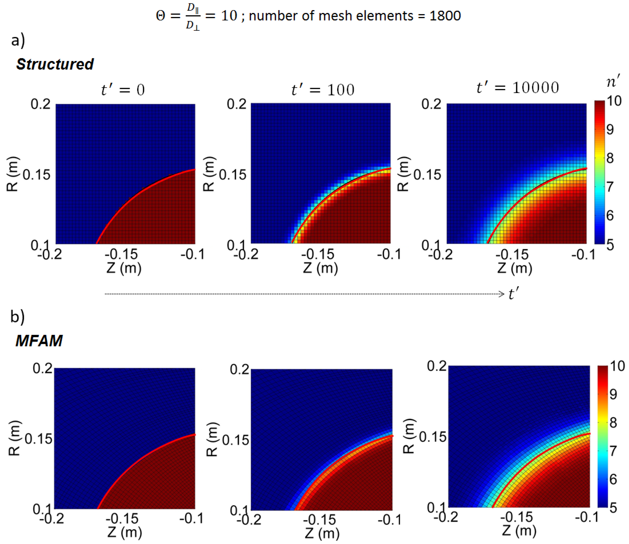
Figure 13 shows a comparison of the solutions of a diffusion problem in two different meshes: A regular and a magnetically aligned meshes with the same number of elements. Once again, the main parameter in the simulation is $\mathrm{\Theta }=D_{\parallel }/D_{\perp }=10$ and the MFAM simulation is solved with a WLSQ method with second order reconstruction polynomial and inverse-distance weighting (which was found to produce the lowest GR errors for this particular case). The errors obtained in the MFAM mesh are found to be smaller than those from the Cartesian one.

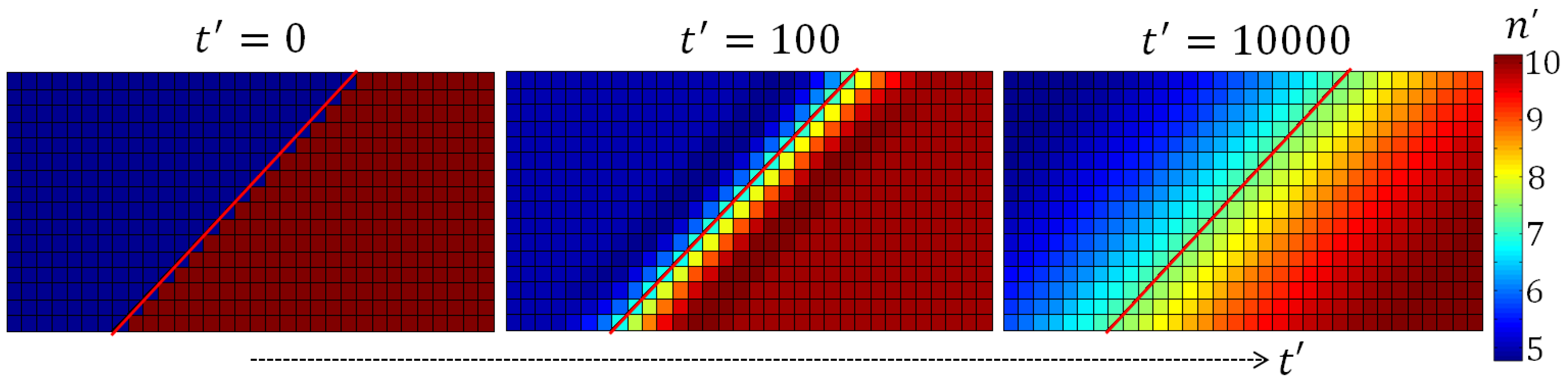
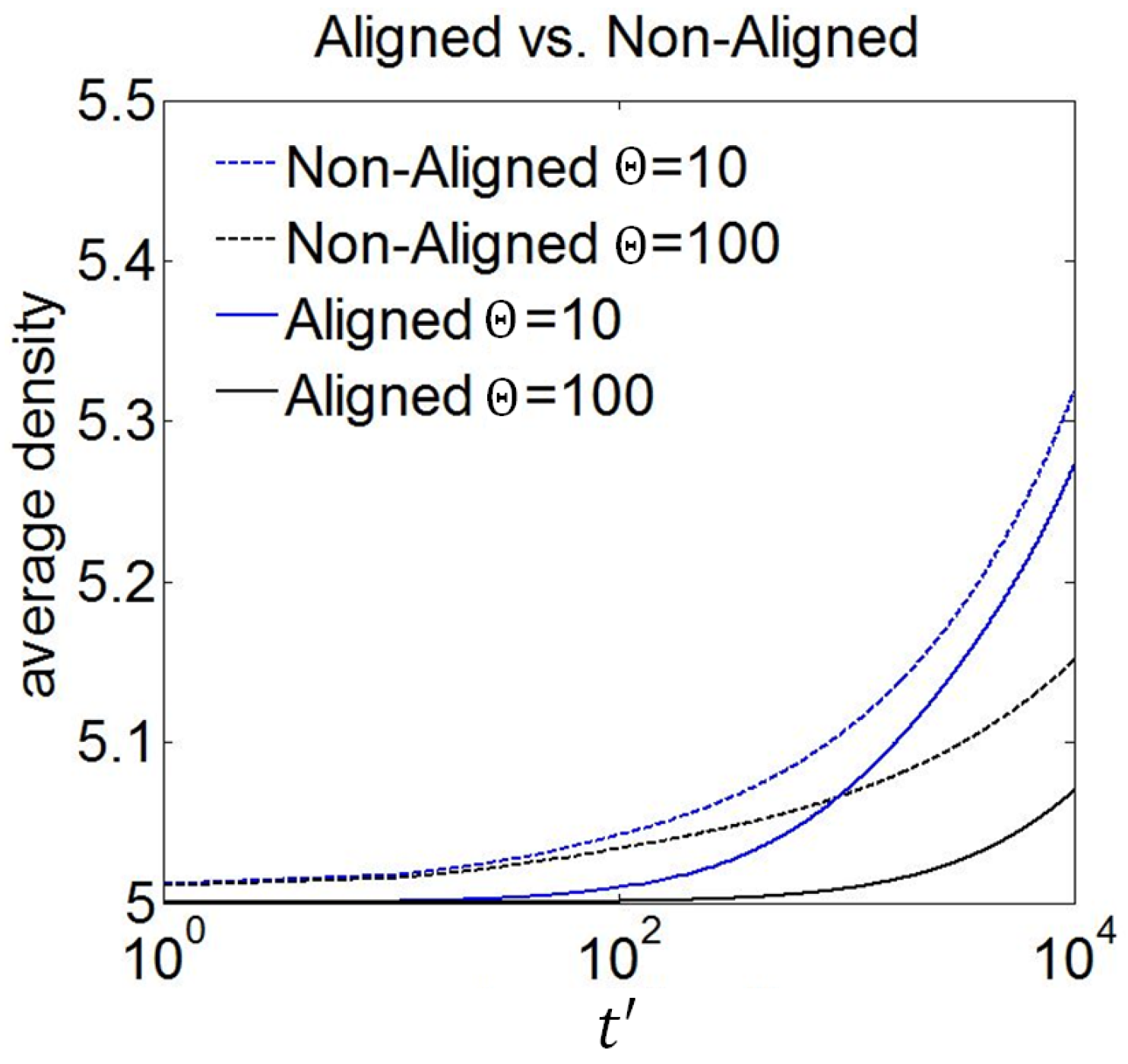
Figure 14 shows the average density evolution in the initial low density region (at $t^{\prime }=0$ in Figure 13, which has been kept as similar as possible between both meshes, accounting for their intrinsic differences) in both meshes and accounts for the difference between the two solutions due to numerical errors. As evidenced by the results, the errors appearing in MFAM are small in comparison to global errors caused by numerical diffusion in the Cartesian mesh and imply that both solutions will diverge for sufficiently large times. Assuming that the simulation for the MFAM is solving the exact diffusion problem, because no numerical diffusion should be present in theory, even if numerical discretization errors are considered, it is demonstrated that, in general, MFAMs offer a solution which is more consistent with the actual evolution problem than the structured mesh for similar mesh refinement. It should be noticed that other discretization errors are still present in MFAMs as can be appreciated in Figure 13. These errors appear due to the truncation of the order on the reconstruction of the Taylor series, the loss of curvature on magnetic mesh lines and the machine rounding, amongst others. In any case these errors will appear in both Cartesian and Curvilinear meshes and so avoiding a key element of numerical diffusion represents an important asset in the selection of MFAM type meshes.

6. Conclusions

The previous sections have shown that large anisotropicities in the diffusion problem are difficult to recover in a Cartesian mesh without extensive refinement of the mesh, which would typically involve large computational resources to solve the problem accurately. In the case of conducting fluids, the use of Magnetic Field Aligned Meshes (MFAMs) helps to solve this problem. These conclusions may be extrapolated to other fluid flows contained in mediums which impose anisotropicity in the problem, such as, for example, non-Newtonian fluids or porous mediums in microfluidic devices or tissues.

For small anisotropicity levels, the relatively smaller numerical diffusion errors might be traded-off against the difficulties of using the non-Cartesian mesh. A first one is that gradient reconstruction in a curvilinear mesh, such as the MFAM, might cause large errors for certain types of solutions (if the implementation or the parameters of the method are incorrectly selected). Then there is the added difficulty of handling a non-Cartesian problem, purely from a coding perspective.

Regarding the example problem shown in this paper, it could be argued that conducting flows, such as plasma discharges in electric propulsion devices happen under complex magnetic topologies (with distinct regions of confinement) and depend greatly on the operating parameters of these devices; this means that prior knowledge of the anisotropicity level in the different transport terms of the governing equations is difficult to attain. Consequently, large refinement of a structured mesh might be needed to deal with numerical diffusion if Cartesian meshes are used. Furthermore, issues in gradient reconstruction may also appear in Cartesian structured meshes if mesh resolution and the order of the method are not selected properly. In the case of MFAMs, various strategies have been presented in this work in order to provide additional confidence on the capability to deal with errors introduced by mesh irregularities.

In light of the results derived above, it can be concluded that the use of curvilinear meshes aligned with the preferential directions of the fluid flow problem in highly anisotropic mediums provides a distinct advantage in bounding numerical errors in the solution, as long as specific challenges in these meshes are taken into account. In particular, the use of MFAMs for the simulation of magnetically confined conducting flows (or specific populations within them), modeled as highly anisotropic fluids, is recommended.

The authors have restricted this work to the use of the WLSQR method as proposed by Sozer due to its proved robustness. The use of hybrid methods, as mentioned along the manuscript, may be considered in the future in order to further refine the quality of Gradient Reconstruction. Other, future work will be oriented toward: (1) adding “attractor points” in MFAM meshing strategies for additional control over mesh refinement, (2) mesh quality improvement methods in boundary elements for problems with non-trivial boundary conditions or (3) the effects over Mesh Quality and Gradient Reconstruction of local element clustering and the use of hanging nodes.