A Fruit Fly-Optimized Kalman Filter Algorithm for Pushing Distance Estimation of a Hydraulic Powered Roof Support through Tuning Covariance

Abstract

To measure the pushing distance of a hydraulic-powered roof support, and reduce the cost from a non-reusable displacement sensor embedded in pushing a hydraulic cylinder, an inertial sensor is used to measure the pushing distance, and a Kalman filter is applied to process the inertial data. To obtain better estimation performance, an improved fruit fly optimization algorithm (IFOA) is proposed to tune the parameters of the Kalman filter, processing noise covariance Q and observation noise covariance R. The key procedures of the proposed method, including state-space model, fitness function, and Kalman filter implementation, are presented. Finally, an artificial signal is utilized to verify the feasibility of the proposed method, and the tuning results of other algorithms, particle swarm optimization (PSO), genetic algorithm (GA), basic FOA, and 3D-FOA are compared. The proposed method is also applied in the pushing distance estimation scenario. The simulation and application results prove the effectiveness and superiority of the proposed method.

1. Introduction

As an essential equipment in a fully-mechanized coal mining working face [1], a hydraulic powered roof support connects with the scraper chain conveyor through the pushing link. Since the cutting machine rides on the scraper chain conveyor, it is evident that the straightness of the scraper chain conveyor directly affects the working efficiency of cutting machine [2], while the straightness is determined by the pushing distance, which is produced by the hydraulic powered roof support. The pushing distance is defined as the distance that the pushing link moves forward or backward. At present, the pushing distance is measured by a displacement sensor which is embedded in the hydraulic pushing cylinder to avoid being exposed in extreme conditions.

However, there are some fatal drawbacks of this approach. The displacement sensor, embedded into the hydraulic pushing cylinder, is non-replaceable due to the cumbersome mechanical structure and its unmaintainable installation method. As a consequence, it will be totally disabled once the sensor is broken, and the sensor cannot be replaced until all of the mining tasks are finished. Moreover, the method has poor accuracy, because the pushing distance is obtained either by using the pushing length of the hydraulic pushing cylinder directly, or calculated via trigonometry transformation. Both of the above methods produce large system errors. Thus, a novel pushing distance estimation approach, with comprehensive consideration of both estimation accuracy and extreme condition constraints, is much needed.

Inertial sensors are widely applied in navigation [3], robotics [4], and virtual reality [5], etc., due to their positive characteristics, such as being lightweight, their low power consumption, portability, and self-contained nature [6]. They were originally proposed for aircraft navigation systems in the 1930s [7]. Later, inertial sensors are growing popular both in scientific research and entertainment technologies. The scientific studies are not limited to applications [8], but also to their performance [9]. Research on their performance improvement [10] and calibration analysis [11] provide more accurate estimation technologies for these interesting applications, e.g., equine lameness examinations [12], human arm motion tracking [13], and quantifying the evaluation of warfighter performance [14], etc. Although inertial sensors are successfully used in many fields, the application on displacement estimation is still a great challenge due to the cumulative errors [15]. As improvements in inertial sensors and rapid development of signal processing methods continue, inertial sensors also provide a possibility for operation in some extreme conditions without accuracy requirements, e.g., a fully-mechanized coal mining working face.

The Kalman filter was proposed for linear filtering and prediction problems by Kalman in 1960 [16]. It is a state estimator based on a state-space model [17]. The Kalman filter is frequently used for inertial information processing due to uncertainty problems [18], including position estimation [19], as well as rotation estimation [20]. For non-linear problems, researchers also proposed some mutation of the Kalman filter, e.g., the extended Kalman filter [21], unscented Kalman filter [22], etc. In recent years, the Kalman filter has also been applied in intelligent computation [23], as well as information fusion through distributed [24] or parallel [25] approaches. In addition to these applications, the Kalman filter contributes to magnetometer calibration [26], moving object tracking [27], and satellite attitude determination [28], as well. Unfortunately, the estimation performance of the Kalman filter is greatly influenced by the selection of the processing covariance matrix Q and the observation (measurement) covariance matrix R [29], and the research on tuning Q and R is very valuable [30]. Thus, optimization algorithms should be applied to obtain better estimation performance through tuning the covariance.

Optimization algorithms have significant influence on computational performance. Recently, some interesting and efficient naturally-inspired optimization algorithms have been proposed. Krill herd (KH) was proposed by Gandomi and Alavi in 2012 [31]. Based on the innovation, other algorithms, such as chaotic KH [32], stud KH [33], hybrid KH [34], chaotic particle-swarm KH [35], multi-stage KH [36], and opposition-based KH [37], etc., are successively developed. These algorithms are so efficient and flexible that they can be improved either by internal improvement, such as introducing a new migration operator [38] and a new information exchange process [39], or by combining other algorithms together, such as quantum-behaved particle swarm algorithms [40] and cuckoo search algorithms [41], etc. Monarch butterfly optimization (MBO) [42] and MBO-based algorithms [43,44] are also recently developed meta-heuristic algorithms, which simulate the migration of monarch butterflies. Other similar algorithms, moth search algorithms [45], earthworm optimization algorithms [46], cuckoo search algorithms [47,48], bat algorithms [49,50] and firefly algorithms [51,52], etc., also simulate the natural motion process and have contributed greatly to intelligent optimization algorithms in recent years.

Among these intelligent optimization algorithms, the fruit fly optimization algorithm (FOA) is a brand new intelligent optimization algorithm, which has a rapid convergence rate and easy implementation, proposed by Pan in 2012 [53]. FOA simulates the intelligent foraging behavior of a fruit fly group in a food-finding process [54], which combines olfactory and vision searching methods [55]. It has been widely applied in financial parameter optimization [56], forecasting [57], scheduling [58], etc. However, like other optimization algorithms, the basic FOA has the possibility of falling into local extremes, and it is difficult to jump out [55].

Bearing the above observations in mind, inertial sensors are utilized to measure the inertial information of a pushing link, and an improved fruit fly algorithm optimized Kalman filter (FOA-KF) is proposed to process the inertial information. To make it easy for jumping out of the local extreme, the basic FOA is modified by adding a perturbation intensity through a predict-update mechanism when falling into a local extreme. A simulation and application for the pushing distance estimation proves the effectiveness and superiority of the proposed method.

The rest of this paper is organized as follows: In Section 2, preliminaries of Kalman filter and basic FOA are presented. In Section 3, the framework of proposed method is described and an improved FOA is applied to optimize the Kalman filter covariance. In Section 4, an artificial inertial signal is estimated to verify the effectiveness and superiority of the proposed method, and an application of pushing distance estimation is performed. Some conclusions and outlooks are summarized in Section 5. Bearing the above observations in mind, an inertial sensor is utilized to measure the inertial information of the pushing link, and an improved fruit fly algorithm optimized Kalman filter (FOA-KF) is proposed to process the inertial information. To make it easier for jumping out of the local extreme, the basic FOA is modified by adding a perturbation intensity through a predict-update mechanism when falling into a local extreme. A simulation and application for the pushing distance estimation proves the effectiveness and superiority of the proposed method.

2. Preliminaries

2.1. Kalman Filter

Generally, the Kalman filter can be described in two stages: firstly, one-step prediction; and secondly, measurement correction. Considering the discrete-time dynamic model of pushing distance estimation, the state vector is $x_k={[p_k,v_k]}^T$, which indicates the current pushing distance and pushing velocity. The observation $y_k$ is the measured displacement. The details of mathematics are described as following steps.

(1) Prediction

The new best estimation is predicted using the previous best estimation (priori estimation), the process equation is:

$${\widehat{x}}_k^{-}=A_k{\widehat{x}}_{k-1}^{+}+B_k{u}_k+w_k$$

(1)

where the state vector ${\widehat{x}}_k^{-}$ is the prior estimation at time k and ${\widehat{x}}_{k-1}^{+}$ is the posterior estimation at time k − 1; $A_k$ is the transition matrix; $B_k$ is control matrix; $u_k$ is the known control input; and $w_k$ is the processing noise, a zero-mean Gaussian processing noise with covariance $Q=E(w_k\cdot w_k^T)$.

Since the processing equation contains processing noise $w_k$. The error covariance matrix of priori estimation is added by processing the noisy covariance matrix, as shown in following equation:

$$P_k^{-}=A_k{P}_{k-1}^{+}{A}_k^T+Q$$

(2)

Similarly, $P_k^{-}$ is the prior error covariance at time k and $P_{k-1}^{+}$ is the posteriori error covariance at time k − 1. The processing noise covariance $Q$ is the processing noise covariance and needs to be tuned.

(2) Correction

The correction stage is essential for refining estimation with measurements. The measurement equation is shown as follows:

$$y_k=H_k{x}_k^{-}+v_k$$

(3)

where $H_k$ is the observation matrix. $v_k$ is the zero-mean Gaussian measurement noise with covariance $R=E(v_k\cdot v_k^T)$. The observation noise covariance $R$ is unknown and waiting for tuning.

To correct estimation with measurement, the Kalman gain is very important to propagate the recursive procedure. The Kalman gain is:

$$K_k=P_k^{-}{H}_k^T{(H_k{P}_k^{-}{H}_k^T+R)}^{-1}$$

(4)

Then, based on the Kalman gain and measurements, the posterior estimation can be calculated as follows:

$${\widehat{x}}_k^{+}={\widehat{x}}_k^{-}+K_k(y-H_k{\widehat{x}}_k^{-})$$

(5)

Finally, the posterior error covariance is reassigned as follows:

$$P_k^{+}=(I-K_k{H}_k)P_k^{-}$$

(6)

The processing noise covariance and observation noise covariance are set through experience, which sometimes leads to large estimation error. To tackle this problem, both $Q$ and $R$ should be optimized via varying estimation algorithms.

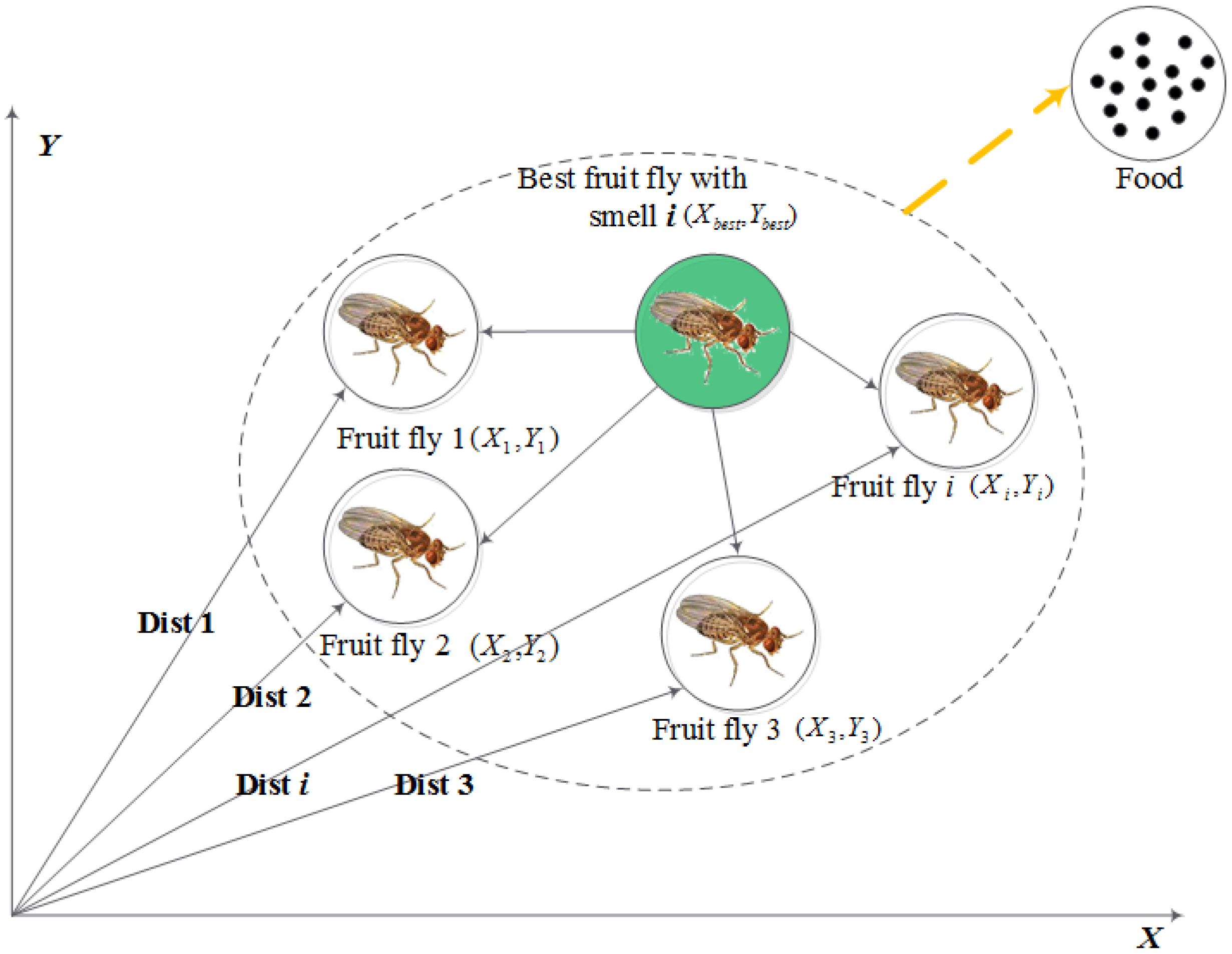
2.2. Fruit Fly Optimization Algorithm

The fruit fly optimization algorithm is inspired by the food-searching mechanism of a fruit fly swarm due to the fact that the fruit fly is superior to other species in vision and osphresis. The fruit flies in a swarm send and receive information from neighbors, compare the current location and fitness, and fly toward the food with better fitness. The global optimization can be obtained via an appropriate iteration, as shown in Figure 1, and the standard foraging process of FOA can be summarized as follows.

Step 1.1: Key initial parameters, population size PS, maximum generation number (maximum iterations) $ite{r}_{\max }$, and location range parameter $LR$ are generated. The initial location of the fruit fly swarm is represented as follows:

$$\{\begin{array}{c}X\_axis=rand(LR)\\ Y\_axis=rand(LR)\end{array}$$

(7)

Step 1.2: Individual fruit fly uses osphresis to search food, and the searching direction is randomly generated as follows:

$$\{\begin{array}{c}X(i)=X\_axis+rand(FR)\\ Y(i)=Y\_axis+rand(FR)\end{array}$$

(8)

where $FR$ is the fruit fly distance range.

Step 1.3: Since the food location cannot be known, the distance to the origin of coordinates $Dis{t}_i$ and the smell concentration judgment value $S_i$ are calculated as follows:

$$\begin{gathered} Dis{t}_i=\sqrt{X_i^2+Y_i^2} \\ {S}_i=\raisebox{1ex}{$1$}\!\left/ \!\raisebox{-1ex}{$Dis{t}_i$}\right. \end{gathered}$$

(9)

Step 1.4: The best fruit fly with maximum smell concentration searches for food according to the smell concentration judgment function (also known as fitness function), which is represented as follows:

$$\begin{gathered} Smell(i)=function(S_i) \\ [bestSmell,bestIndex]=\max (Smell) \end{gathered}$$

(10)

where $bestSmell$ denotes the maximal smell concentration, $bestIndex$ is the corresponding fruit fly number, and $Smell$ is the smell concentration set of the group.

Step 1.5: Compare the smell concentration with the previous best smell concentration; if it is better than the last generation, update the current best location as follows:

$$\begin{gathered} SmellBest=bestSmell \\ \{\begin{array}{c}X\_axis=X(bestIndex)\\ Y\_axis=Y(bestIndex)\end{array} \end{gathered}$$

(11)

Otherwise, go back to Step 1.2 to find other better smell concentrations.

Step 1.6: If the searching process reaches the maximum generation number, the procedure will be terminated, otherwise, repeat Step 1.2 to Step 1.5. This optimization algorithm is very efficient to reach the global optimization, but it is also easy to fall into a local optimization.

3. Proposed Method

In this section, an improved FOA (IFOA) is proposed to avoid falling into a local extremum. The IFOA is applied to tune the parameters of the Kalman filter, i.e., processing noise covariance $Q$ and observation noise covariance $R$. The whole procedure of pushing distance estimation based on the fruit fly algorithm-optimized Kalman filter (IFOA-KF) is presented.

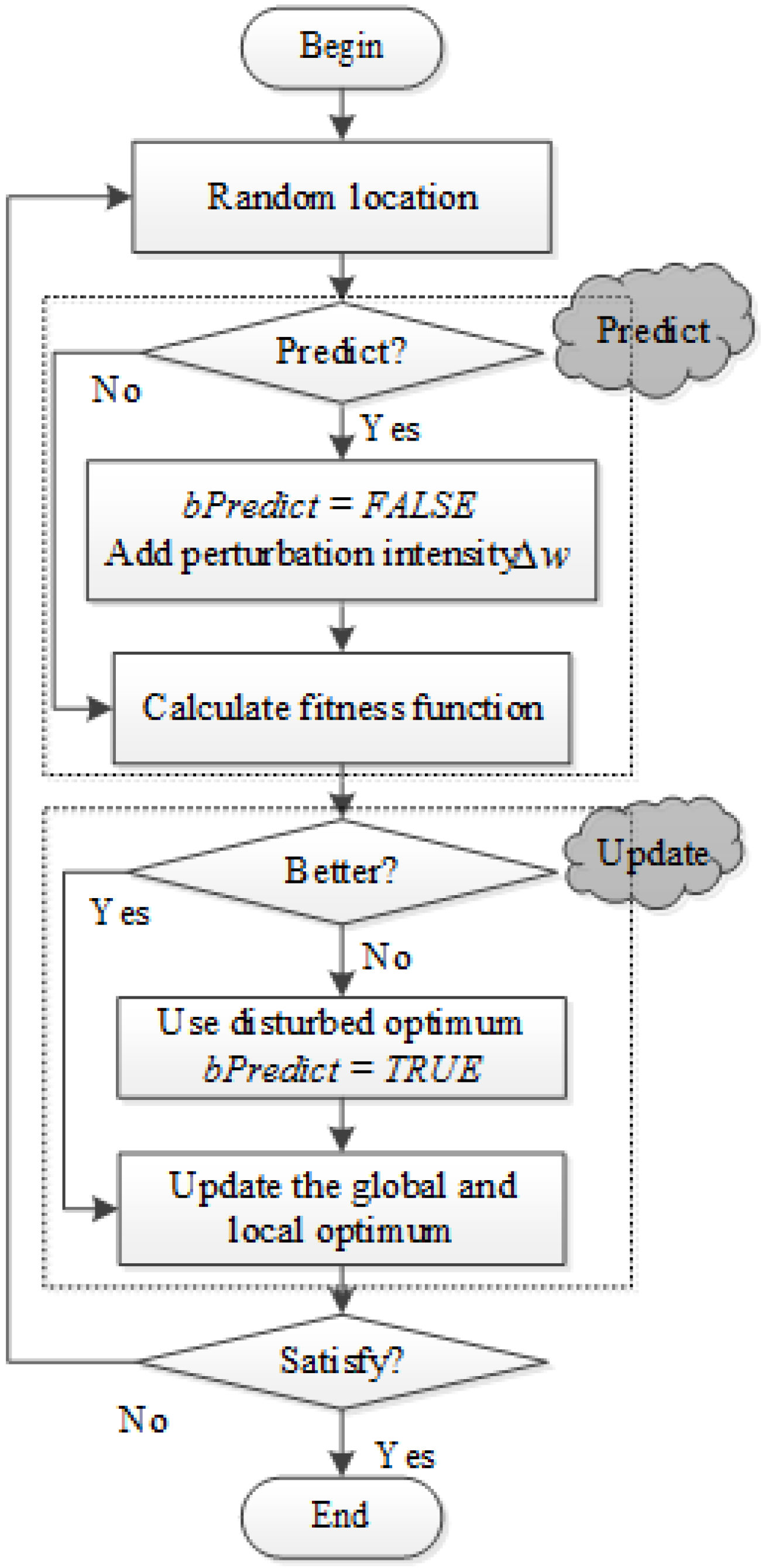
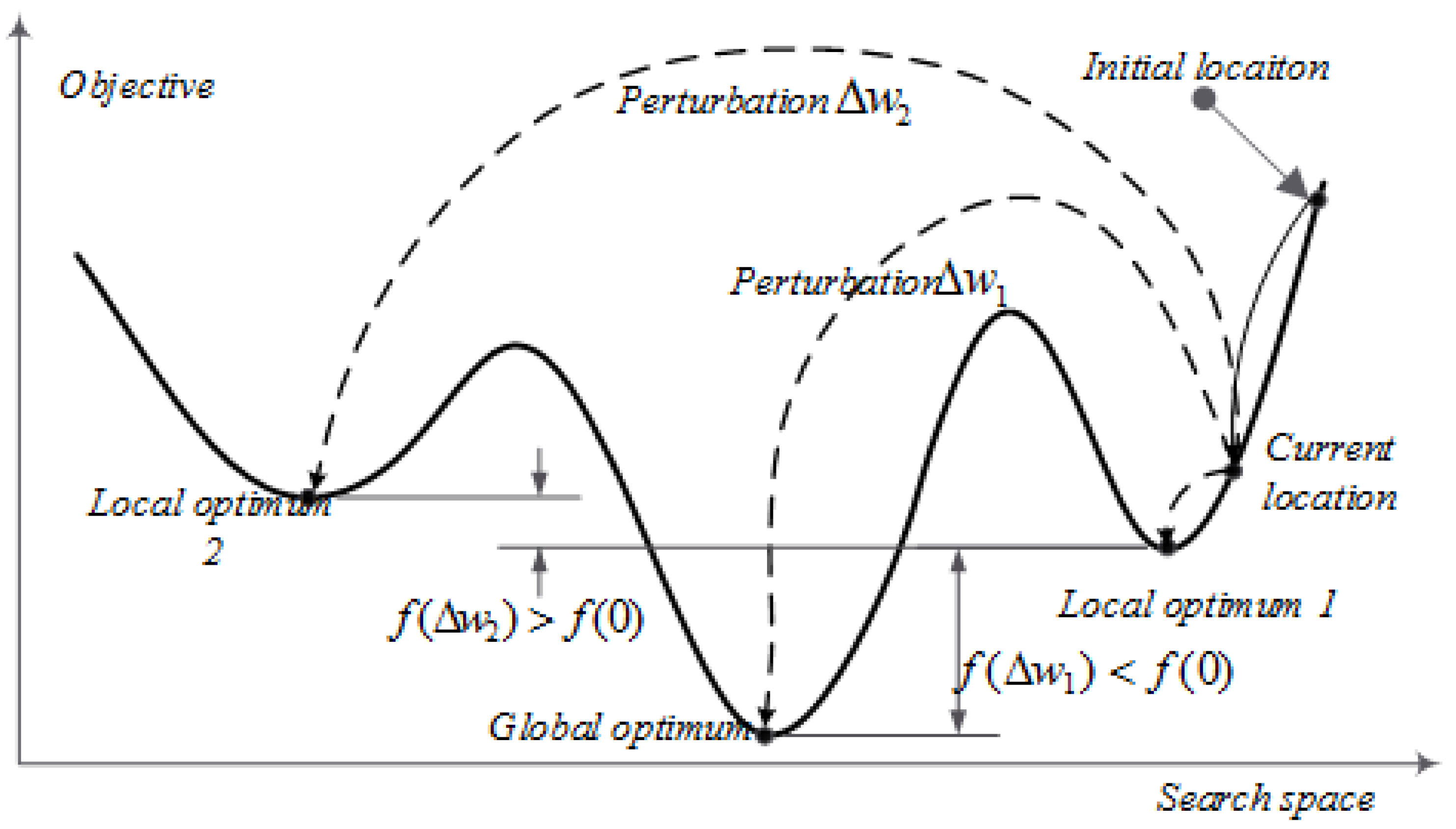
3.1. The Proposed IFOA

The basic FOA is very efficient in finding the global optimization, while it is a common problem to fall into local extremum. To tackle this problem, Wang [59] adds a random perturbation to jump out of the local extremum, while the perturbation intensity is chosen randomly. Suppose that the basic FOA may fall into local optimum 1, as shown in Figure 2: a perturbation with high intensity may change the current location to another local optimum 2. While an appropriate perturbation intensity may reach to global optimum.

In order to tackle this problem, the proposed IFOA utilizes a predict-update mechanism to determine if the perturbation intensity should be added or not. If the flag variable $bPredict$ is true, the proposed IFOA should add the perturbation and predict the next location. If the flag variable $bPredict$ is false, then go directly to the next step. To set the flag variable, the objective values with or without perturbation intensity should be compared. If the objective with perturbation intensity is better, then apply this perturbation intensity. If not, then set current perturbation intensity to zero, namely, without perturbation intensity. Thus, the perturbation intensity can be chosen via the following conditions:

$$\Delta w=\{\begin{array}{ll}0,\hfill & f(\Delta w)\ge f(0)\\ \Delta w,\hfill & f(\Delta w)<f(0)\end{array}$$

(12)

where $f(\cdot )$ is the objective function to be minimized. As shown above, if random perturbation $\Delta w=\Delta w_1$, and $f(\Delta w_1)<f(0)$, then the predicted random perturbation can be accepted and added to the current location, the next location may be a point near the global optimum or another local optimum. If random perturbation $\Delta w=\Delta w_2$, and $f(\Delta w_2)>f(0)$, then the predicted random perturbation can be rejected, which means the procedure just uses the original location. By recursive execution of this step, the final global optimum will be located. To adaptively set the perturbation intensity, varying adaptive methods can be applied, while this is beyond the research scope of the paper. Finally, the flowchart of IFOA is shown in Figure 3, and the whole procedure contains two parts: predict and update. The algorithm can be described in the following steps.

Step 2.1: Initialize all of the parameters, maximum iterative steps, population size, and location range of the fruit fly group, as well as the initial perturbation intensity $\Delta w$.

Step 2.2: Randomly choose the location of the fruit fly group, and check the flag of the prediction procedure which indicates whether the random perturbation should be used. If using the prediction procedure, reset the flag, and add the perturbation with intensity $\Delta w$. If not, go directly to the next step.

Step 2.3: Obtain a smell concentration judgment, and calculate the fitness function using the original distance with or without perturbation.

Step 2.4: If the result of the fitness produced using the original distance with perturbation is better, update the current location of individuals by the disturbed locations. Otherwise, skip to the next step.

Step 2.5: If the fitness value from the fruit fly with the best smell is better than that of the previous generation, then the global and local optimum can be updated. Otherwise, set the prediction flag to TRUE, and update the global and local optimum.

Step 2.6: If the current iterative procedure output meets the requirement, stop the searching process; if not, go back to Step 2.2.

From the figure and the above description, the prediction procedure, which determines the perturbation intensity, can be implemented from Step 2.2 to Step 2.3, and the update procedure, which updates the current location with the predicted perturbation intensity, can be implemented through Step 2.4 to Step 2.5.

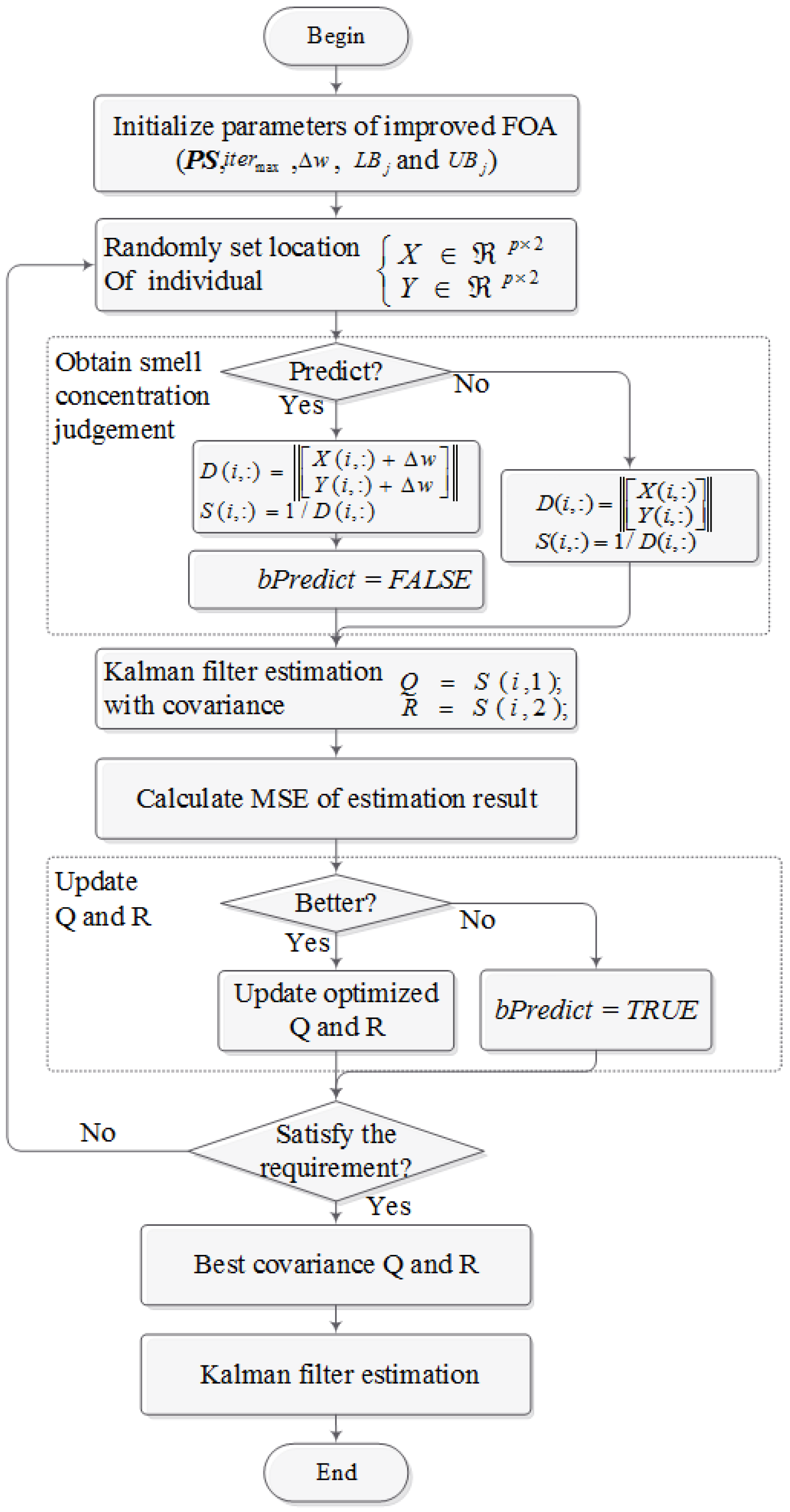
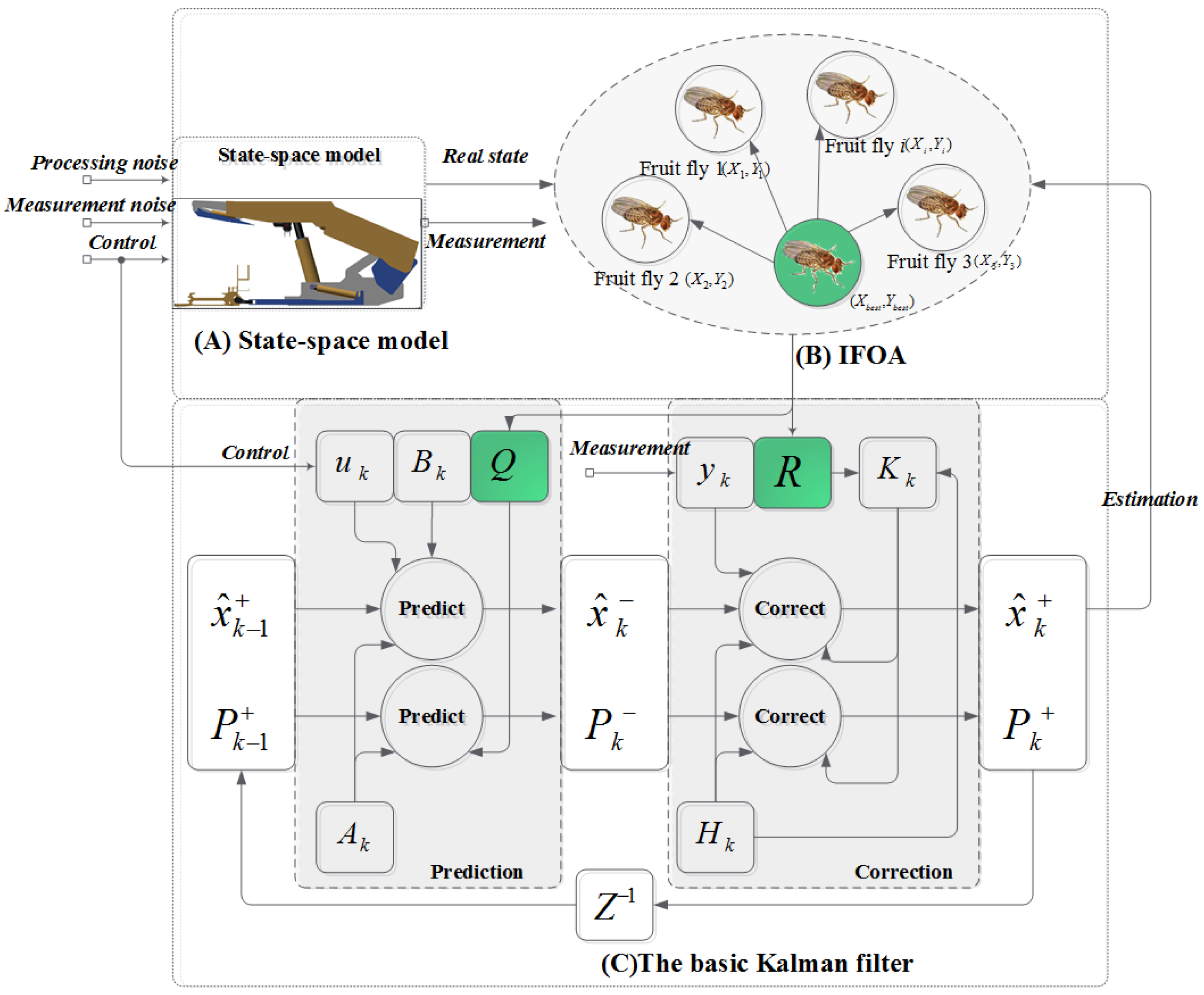
3.2. The Optimized Kalman Filter Based on IFOA(IFOA-KF)

The tuning parameters, processing noise covariance $Q$, and observation noise covariance $R$ indicate the uncertainty of the prediction model and the correction model, respectively. Both the processing noise covariance and observation noise covariance are unknown and need to be tuned for better estimation performance. $Q$ is notoriously difficult but it helps to inject uncertainty into the state equations and assist the filter to learn from the measurement. There are three different options for $Q$ tuning: (1) scalar quantity; (2) diagonal matrix; and (3) full matrix. In this paper, since the processing noise is mainly contributed by acceleration [60], $Q$ is optimized as a scalar quantity. Observation matrix $H_k$ is a vector because the measured variable is the current pushing distance, thus, $R$ is also a scalar quantity. As shown in Figure 4, the offline Kalman filter tuning procedure based on IFOA is presented, and the block diagram of the proposed method can be described as follows.

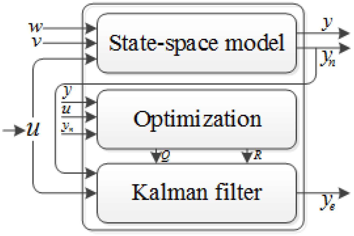
(1) State-Space Model

Firstly, the state-space model of pushing distance estimation, as shown in Figure 4A, should be constructed. The state-space model can be represented by two equations: a processing equation and an observation equation. The processing equation of pushing distance estimation is obtained as follows:

$$\begin{gathered} p_k=p_{k-1}+\Delta t\cdot v_{k-1}+\frac{1}{2}{a}_k\Delta t^2 \\ {v}_k=v_{k-1}+a_k\Delta t \end{gathered}$$

(13)

By linearization of above equation and comparing it with Equation (2), parameters of the processing model can be constructed. $A_k=\left[\begin{array}{cc}1& \Delta t\\ 0& 1\end{array}\right]$, $B_k=\left[\begin{array}{c}\raisebox{1ex}{$1$}\!\left/ \!\raisebox{-1ex}{$2$}\right.\Delta t^2\\ \Delta t\end{array}\right]$ and $u_k$ is the acceleration $a_k$.

Since the only measurable state variable is displacement $p_k$, the observation equation is shown as follows:

$$y_k=\left[\begin{array}{cc}1& 0\end{array}\right]\left[\begin{array}{c}{p}_k\\ v_k\end{array}\right]$$

(14)

Then, the observation matrix is vector $H_k=\left[\begin{array}{cc}1& 0\end{array}\right]$.

(2) Fitness Function

As analyzed in Section 4.1, to apply IFOA in pushing distance estimation, the fitness function is the key point to tune the Kalman filter. In this paper, the fitness function is obtaining a better set of $Q$ and $R$ values resulting in lower mean squared error from the output of the Kalman filter. Thus, the fitness function of the tuning process is calculated as follows:

$$f_{\min }=\Vert x_k^{+}-x\Vert =E\left[\left(x_k^{+}-x\right){\left(x_k^{+}-x\right)}^T\right]$$

(15)

where $x_k^{+}$ is the current posterior estimation of the pushing distance, $x$ is the real state of the pushing distance estimation system, and $E(\cdot )$ are expectation operations, which obtain the sum of the mean squared error.

(3) Kalman Filter

The block diagram, as shown in Figure 4C, shows all of the procedures of a basic Kalman filter. In this paper, the acceleration signal obtained through the inertial sensor is treated as the control input $u_k$. The measured displacement obtained through the built-in electro-hydraulic control system of the hydraulic powered roof support is the observable variable $y_k$. During the parameter tuning process, the estimated state produced by the Kalman filter and the real state produced by the state-space model go through the fitness function, and obtain the mean square error. The mathematical description of the Kalman filter is presented as Equation (1) to Equation (6).

The flowchart of the proposed method, as shown in Figure 5, is presented and the pseudo-code is demonstrated as follows:

Procedure: IFOA-KF

Parameters: PS, $ite{r}_{\max }$, $\Delta w$, $L{B}_j$, $U{B}_j$

Outputs: Q,R

% Initialization

Set population size PS, maximum generation $ite{r}_{\max }$, and perturbation intensity $\Delta w$ and $L{B}_j$, $U{B}_j$

%Set random initial position of fruit fly swarm

For i = 1, 2,…, PS

$[X(i,:),Y(i,:)]=L{B}_j+(U{B}_j-L{B}_j)\times rand(1,2);$

End

${\Delta }_{Q,R}\leftarrow \underset{i=1,2,\dots ,PS}{\min }\left(MSE\left(X(i,:),Y(i,:)\right)\right)$ %Set individual with best smell concentration

$[X\_axis,Y\_axis]={\Delta }_{Q,R}$

For j = 1: $ite{r}_{\max }$

% if prediction is enabled

If bPredicte == TRUE then bPredicte = FALSE

$[X\_axis,Y\_axis]=[X\_axis,Y\_axis]+\Delta w\times rand(1,2);$

End

For i = 1, 2,…, PS

% Random direction and distance

$[X(i,:),Y(i,:)]=[X\_axis,Y\_axis]+(U{B}_j-L{B}_j)\times rand(1,2);$

If $[X(i,:),Y(i,:)]>U{B}_j$ then $[X(i,:),Y(i,:)]=U{B}_j$

If $[X(i,:),Y(i,:)]<L{B}_j$ then $[X(i,:),Y(i,:)]=L{B}_j$

% obtain smell concentration

$S(i,:)=1/Dist\left((X,Y)\right)$

% MSE of Kalman filter estimation result

$Smell(i)=MSE(Kalman(S(i,:)))$

End

$Bes{t}_{Q,R}=\underset{i=1,2,\dots ,PS}{\min }\left(Smell\right)$

If $Bes{t}_{Q,R}\le {\Delta }_{Q,R}$ then ${\Delta }_{Q,R}=Bes{t}_{Q,R}$

If $Bes{t}_{Q,R}>{\Delta }_{Q,R}$ then bPredicte = TRUE

% Kalman filter estimation using best covariance

$results=Kalman(Bes{t}_{Q,R})$

END

Where, $Dist(\cdot )$ is the operation to obtain the distance from the current fruit fly location to the original coordinate; $MSE(\cdot )$ is the mean squared error of the estimation results; $Kalman(\cdot )$ is the Kalman estimation operation presented as Equation (1) to Equation (6); $L{B}_j$ and $U{B}_j$ are the lower and upper boundaries of location range, respectively.

4. Simulation and Application

In this section, the proposed IFOA-KF is applied to a simulation with an artificial signal. The application of pushing distance estimation is demonstrated as well.

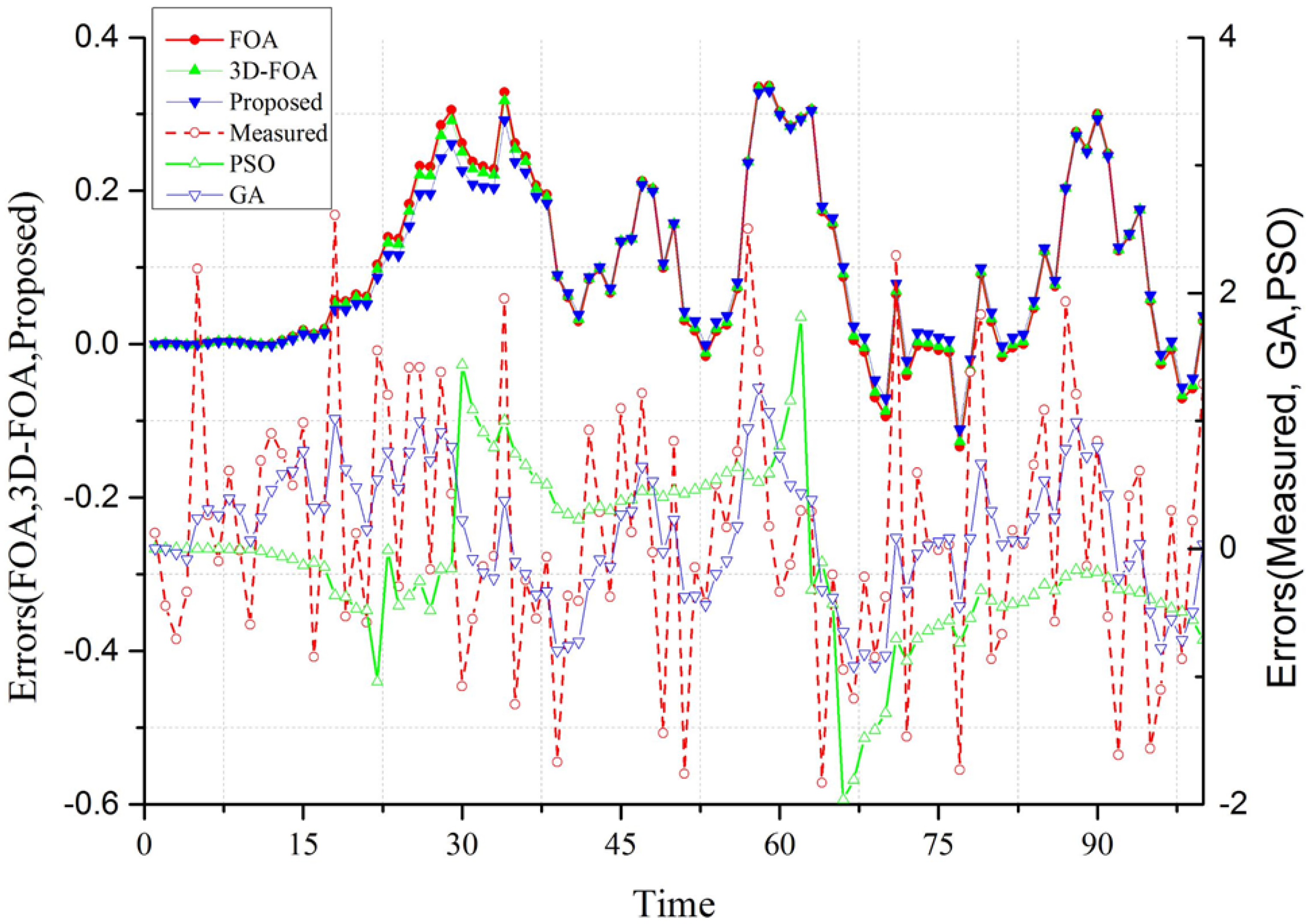
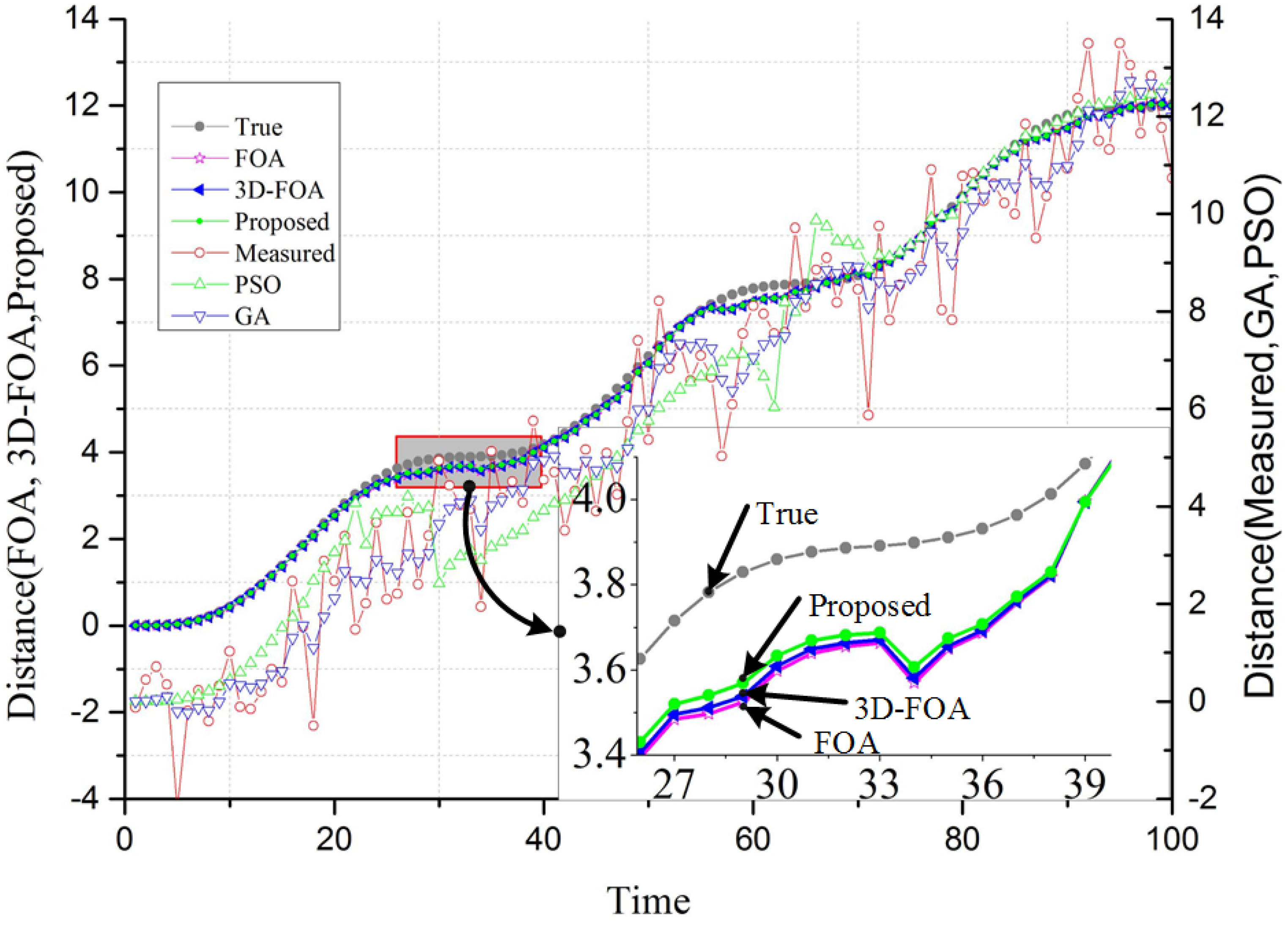
4.1. Simulation with an Artificial Signal

For this simulation, we attempt to track the pushing distance with a Kalman filter, whose covariance Q and R are optimized by different optimization algorithms, e.g., a particle swarm optimization (PSO), genetic algorithm (GA), basic fruit fly algorithm (FOA), and 3D fruit fly algorithm (3D-FOA).

Firstly, the parallel model for pushing distance tracking is constructed using MATLAB (Matlab 2016b, Torrance, CA, USA), as shown in following Figure 6. The input acceleration is a sinusoidal function: $u_k=g\cdot \sin (\raisebox{1ex}{$k$}\!\left/ \!\raisebox{-1ex}{$5$}\right.)$, where $g$ is a constant variable and given as $g=9.81$. We simulate the process noise $w$ and measurement noise $v$ with random functions. Then, the simulated parameters go through the parallel plant model based on the state-space model described in Equations (12) and (13). The true output of the model is $y$, the measurement with measurement noise is $y_n$, and the estimation using the Kalman filter is $y_e$.

Secondly, create the fitness function, which utilizes the above parallel model to simulate the measurement and estimation. Then calculate the mean squared error using Equation (12).

Finally, the simulation results can be obtained via the following configurations, which is listed in following

Table 1. Simulation configurations.

Index	Configuration
Processor	Intel Core i7, 2.5 GHz
RAM	8 G
System	Win 10, x64
Software	MATLAB

:

For comparison, four other optimization algorithms are also implemented and the comparison of the results are shown in

Table 2. Comparison of the estimation results produced by different algorithms.

Algorithms	MSE	Time (s)
PSO	0.39747	7.7298
GA	0.26777	13.002
FOA	0.022869	7.0885
3D-FOA	0.022089	7.3534
Proposed IFOA	0.020527	7.2502

.

In this simulation, the parameters set for the FOA and 3D-FOA are the same. Some key parameters are given: maximum generations is 100, population size is 20, location range is [−1.0, 1.0], and food range is [−3.1, 3.1], etc. For the proposed IFOA, all of the parameters are the same as the FOA and 3D-FOA except the perturbation intensity $\Delta w$. In this simulation, perturbation intensity is given as a fixed value 3.1. To complete the optimization using GA, the MATLAB genetic algorithm toolbox is used, and the function (GAOPTIMSET) is utilized to set all of the options about GA evolution. For the simulation using PSO, import parameters should also be set properly, and the details about the parameters are listed in

Table 3. Parameters.

GA		PSO
Parameter	Value	Parameter	Value
Generations	100	Generations	100
Population size	20	Population size	20
Initial Population	[2, 2]	Particle length	2
Crossover Fraction	0.8	Population range	[−5, 5]
Migration Fraction	0.2	Velocity range	[−1, 1]
Function to corssover	crossoverarithmetic	Acceleration coefficients	[1.49445, 1.49445]
Function for mutation	mutationadaptfeasible	Inertia weight factor	0.729

.

The proposed FOA obtained the minimal mean squared error (MSE) (0.020527), while GA and PSO obtained larger errors, and their calculation time is rather larger than the other three algorithms based on FOA. Especially, the basic FOA is the fastest, but is subtly rough to find the global optimal compared to the proposed method and 3D-FOA. Compared to 3D-FOA, the proposed FOA performed better both in the estimation accuracy and the computational time, since the covariances are optimized offline. Despite the proposed FOA being more complex than the basic FOA, it is still the best choice after a comprehensive tradeoff.

The estimation results of the pushing distance, as displayed in Figure 7, show that FOA, 3D-FOA, and the proposed FOA perform much better than PSO and GA, which is presented in the bottom-right due to the different magnitude of the estimated pushing distance. From the pushing distance estimation results, the difference between FOA, 3D-FOA, and the proposed FOA are not obvious. While the estimation errors, as shown in Figure 8, are capable of revealing the difference, the estimation errors of GA and PSO, as shown in the bottom-right figure, are quite large (MSE of GA PSO are 0.26777 and 0.39747, respectively). The proposed FOA, with the lowest MSE = 0.020527, is the most efficient.

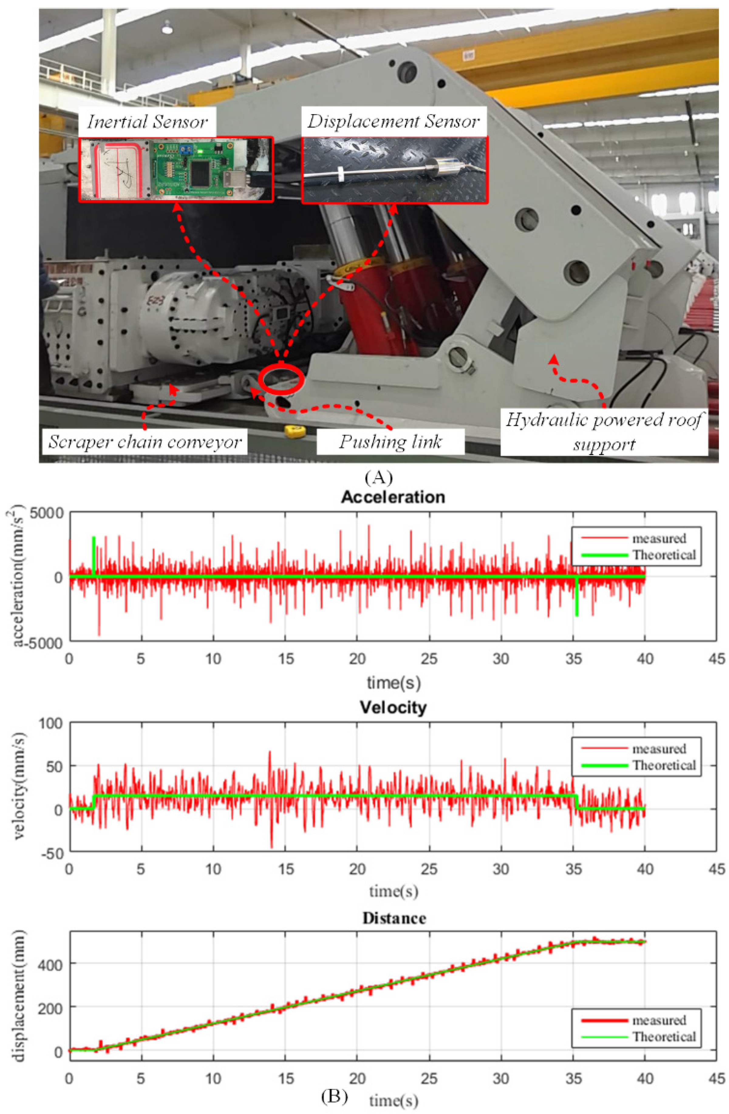
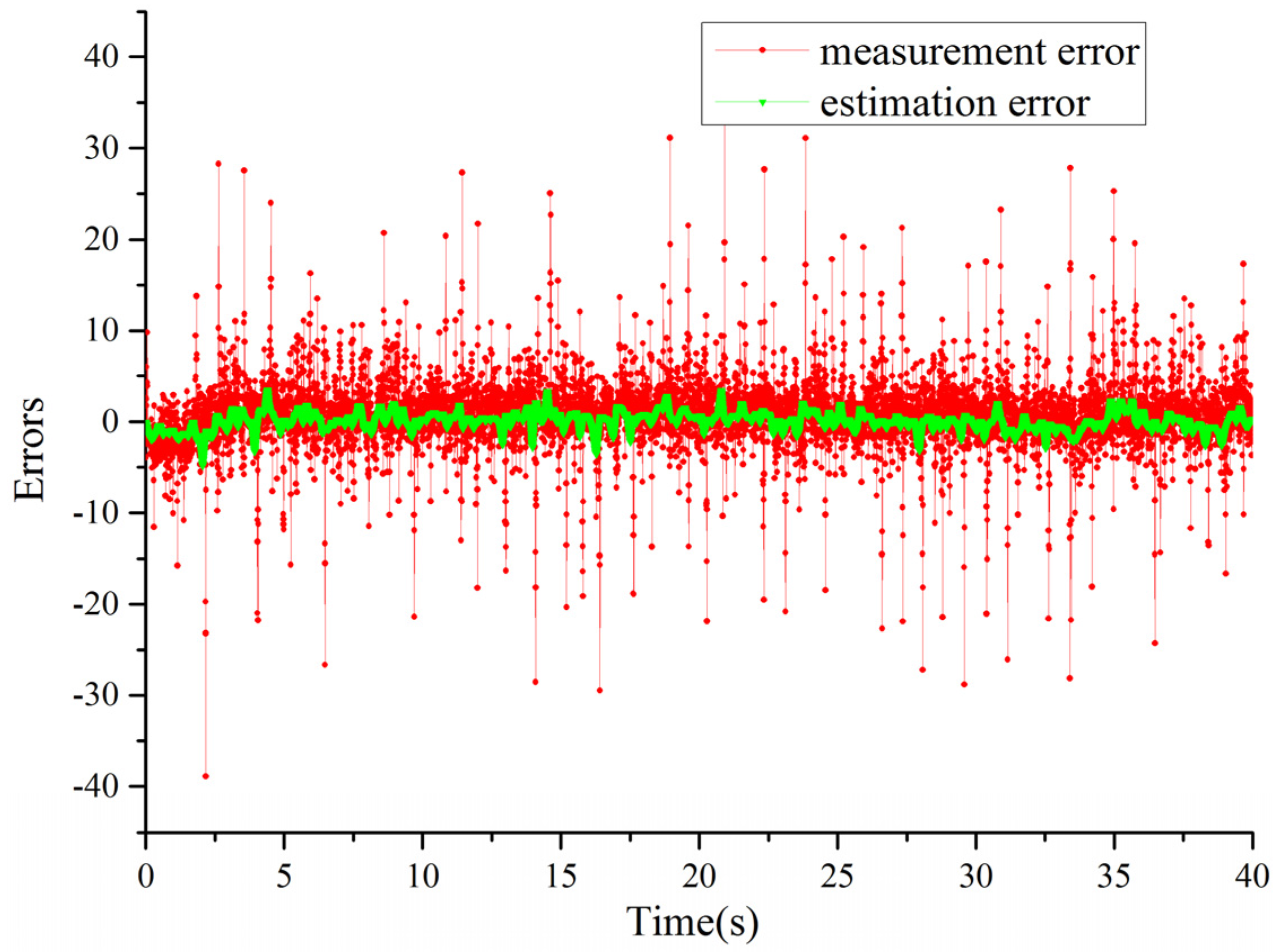
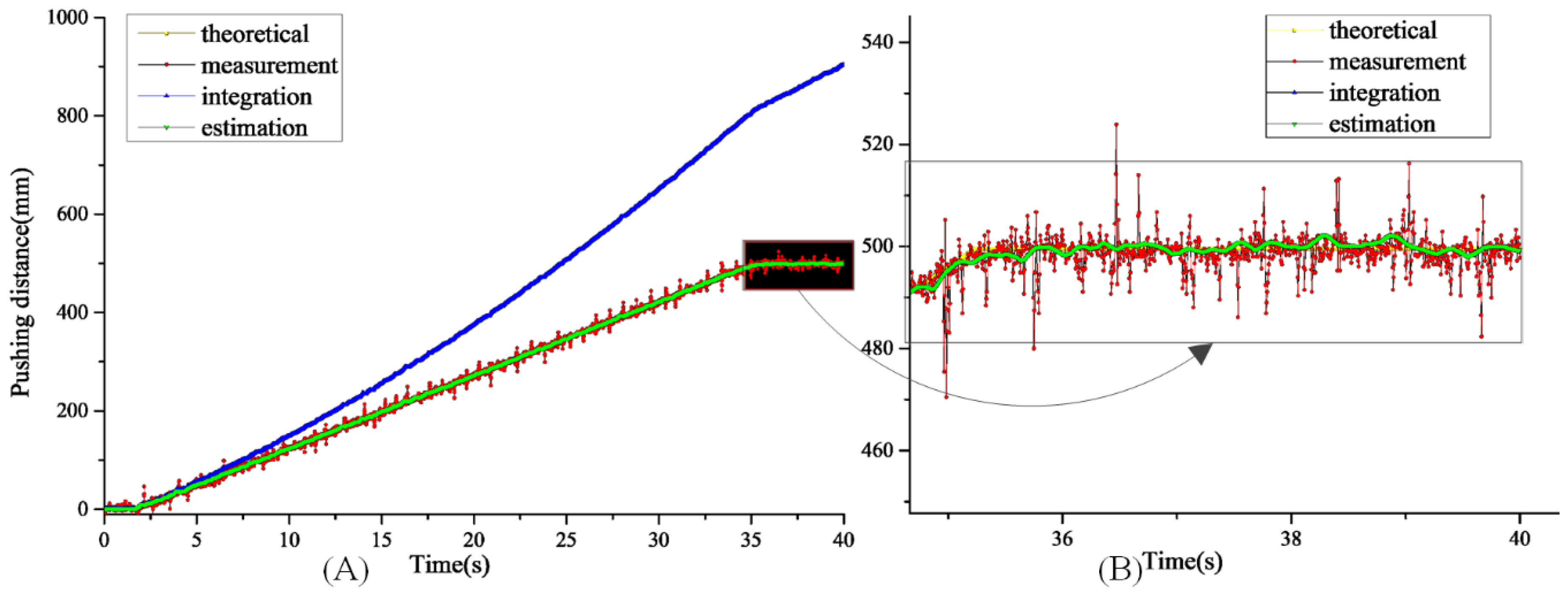
4.2. Application in Pushing Distance Estimation

In addition to the simulation, the proposed method is also applied to the application of pushing distance estimation, based on the real parameters of the hydraulic pushing cylinder, theoretically, the velocity and the pushing distance of the pushing link. In this application, we use a high-precision displacement sensor to measure the pushing distance. The built-in electro-hydraulic control system of a hydraulic powered roof support is used to obtain the observable pushing distance. An inertial sensor is used to measure the inertial information of the pushing link. The detail of the equipment configuration is shown in

Table 4. Equipment configuration.

Index	Equipment	Information
1	Hydraulic powered roof Support	ZY9000/15/28D
2	Displacement sensor	PR-500 mm
3	Data acquisition card	Smacq USB-4432
4	Inertial Sensor	ADIS 16448

.

The inertial sensor, as shown in Figure 9A, is mounted on the pushing link, and the displacement sensor is installed along the direction of pushing operation. The theoretical pushing distance, velocity, and acceleration, as shown in Figure 9B, reveals the basic movement features of the pushing distance. The measured pushing distance from the high-precision displacement sensor, computed velocity via differential equation, and the measured acceleration by the inertial sensors are also presented.

Through the proposed IFOA-KF, the measured acceleration can be used to estimate pushing distance, as shown in Figure 10. The IFOA optimized the processing and observation covariance, and the final optimized parameters are listed in

Table 5. Optimized parameters.

Covariances	Values
Q	0.1758
R	0.4935

.

For a pushing operation of the hydraulic powered roof support, the maximum pushing distance, theoretically, should be 500 mm, as shown in Figure 10A. If the proposed IFOA-KF is not utilized, the directly computational result (the blue curve) will be terribly affected by cumulative errors, and the estimated pushing distance increases rapidly to an unreasonable magnitude. By using the proposed IFOA-KF, the estimated pushing distance, the green curve, is rather close to the real measured pushing distance. Figure 10B also presents the details of the estimation performance at the final stage of the pushing operation. It can be seen that the cumulative error is very limited.

With careful design of the application conditions, the final estimation error can be perfectly reduced; as shown in Figure 11, the error of measurement is 14.7467, while the estimation error of the proposed IFOA-KF is only 1.0425. Thus, the application proves the special performance of the proposed method.

5. Conclusions and Future Work

To tackle the measurement problem of the pushing distance for a hydraulic-powered roof support, this paper proposed an improved fruit fly optimization algorithm (IFOA) to fine-tune processing the noise covariance and observation noise covariance of a Kalman filter, and the optimized Kalman filter is applied to estimate the pushing distance. In the proposed IFOA, the perturbation with a certain intensity is added to the current searching location to avoid the local optimum. Moreover, the flowchart of the IFOA is presented, and the details, state-space model, fitness function, and Kalman filter implementation procedure are demonstrated. To verify the performance of the proposed method, other optimization algorithms (GA, PSO, basic FOA, and 3D-FOA) are utilized to process a simulated artificial signal. A comparison of the results proved the effectiveness and superiority of the proposed method. Finally, the proposed IFOA-KF is applied for pushing distance estimation, and the estimation results also proved the state-of-art performance of the proposed IFOA-KF.

This work is very valuable for pushing distance estimation, and solves the problem of a non-reusable displacement sensor on a fully-mechanized coal mining working face. However, the error elimination is still a challenge. Our future work will focus on optimization of the error elimination, and applying this approach to other similar scenarios, such as inertial sensor information estimation, Kalman-based position tracking, and supporting height estimation of hydraulic supports, etc.

References

1. Wang, J. Present status and development tendency of fully mechanized coal mining technology and equipment with high cutting height in China. Coal Sci. Technol. 2006, 34, 4–7. [Google Scholar]
2. Gong, X.; Ma, X.; Zhang, Y.; Yang, J. Application of fuzzy neural network in fault diagnosis for scraper conveyor vibration. In Proceedings of the 2013 IEEE International Conference on Information and Automation (ICIA), Yinchuan, China, 26–28 August 2013; pp. 1135–1140.
3. Brown, A.K. GPS/INS uses low-cost MEMS IMU. IEEE Aerosp. Electron. Syst. Mag. 2005, 20, 3–10. [Google Scholar] [CrossRef]
4. Lee, T.; Shin, J.; Cho, D. Position estimation for mobile robot using in-plane 3-axis IMU and active beacon. In Proceedings of the 2009 IEEE International Symposium on Industrial Electronics, Seoul, Korea, 5–8 July 2009; pp. 1956–1961.
5. Steinbis, J.; Hoff, W.; Vincent, T.L. 3D Fiducials for Scalable AR Visual Tracking. In Proceedings of the International Symposium on Mixed and Augmented Reality, Cambridge, UK, 15–18 September 2008; pp. 183–184.
6. Sprager, S.; Juric, M. Inertial Sensor-Based Gait Recognition: A Review. Sensors 2015, 15, 22089–22127. [Google Scholar] [CrossRef] [PubMed]
7. Ahmad, N.; Ghazilla, R.A.R.; Khairi, N.M.; Kasi, V. Reviews on Various Inertial Measurement Unit (IMU) Sensor Applications. Int. J. Signal Proc. Syst. 2013, 256–262. [Google Scholar] [CrossRef]
8. Chen, Z.H.; Zhu, Q.C.; Soh, Y.C. Smartphone Inertial Sensor-Based Indoor Localization and Tracking With iBeacon Corrections. IEEE Trans. Ind. Inform. 2016, 12, 1540–1549. [Google Scholar] [CrossRef]
9. Zhong, M.Y.; Guo, J.; Yang, Z.H. On Real Time Performance Evaluation of the Inertial Sensors for INS/GPS Integrated Systems. IEEE Sens. J. 2016, 16, 6652–6661. [Google Scholar] [CrossRef]
10. Wu, Y.X.; Luo, S.T. On Misalignment between Magnetometer and Inertial Sensors. IEEE Sens. J. 2016, 16, 6288–6297. [Google Scholar] [CrossRef]
11. Abruzzo, B.A.; Recchia, T.G. Online Calibration of Inertial Sensors for Range Correction of Spinning Projectiles. J. Guid. Control Dyn. 2016, 39, 1918–1924. [Google Scholar] [CrossRef]
12. Rettig, M.J.; Leelamankong, P.; Rungsri, P.; Lischer, C.J. Effect of sedation on fore- and hindlimb lameness evaluation using body-mounted inertial sensors. Equine Vet. J. 2016, 48, 603–607. [Google Scholar] [CrossRef] [PubMed]
13. Atrsaei, A.; Salarieh, H.; Alasty, A. Human Arm Motion Tracking by Orientation-Based Fusion of Inertial Sensors and Kinect Using Unscented Kalman Filter. J. Biomech. Eng.-Trans. ASME 2016, 138. [Google Scholar] [CrossRef] [PubMed]
14. Davidson, S.P.; Cain, S.M.; McGinnis, R.S.; Vitali, R.R.; Perkins, N.C.; McLean, S.G. Quantifying warfighter performance in a target acquisition and aiming task using wireless inertial sensors. Appl. Ergon. 2016, 56, 27–33. [Google Scholar] [CrossRef] [PubMed]
15. Coyte, J.L.; Stirling, D.; Ros, M.; Du, H.; Gray, A. Displacement profile estimation using low cost inertial motion sensors with applications to sporting and rehabilitation exercises. In Proceedings of the 2013 IEEE/ASME International Conference on Advanced Intelligent Mechatronics: Mechatronics for Human Wellbeing, Wollongong, Australia, 9–12 July 2013; pp. 1290–1295.
16. Kalman, R.E. A New Approach to Linear Filtering and Prediction Problems. ASME Trans. J. Basic Eng. 1960, 82, 35–45. [Google Scholar] [CrossRef]
17. Ljung, L. Asymptotic-behavior of the extended Kalman filter as a parameter estimator for linear-systems. IEEE Trans. Autom. Control 1979, 24, 36–50. [Google Scholar] [CrossRef]
18. Deng, Z.A.; Hu, Y.; Yu, J.G.; Na, Z.Y. Extended Kalman Filter for Real Time Indoor Localization by Fusing WIFI and Smartphone Inertial Sensors. Micromachines 2015, 6, 523–543. [Google Scholar] [CrossRef]
19. Urrea, C.; Munoz, R. Joints Position Estimation of a Redundant Scara Robot by Means of the Unscented Kalman Filter and Inertial Sensors. Asian J. Control 2016, 18, 481–493. [Google Scholar] [CrossRef]
20. Liu, L.J.; Qi, B.; Cheng, S.M.; Xi, Z.R. High precision estimation of inertial rotation via the extended Kalman filter. Eur. Phys. J. D 2015, 69. [Google Scholar] [CrossRef]
21. Plett, G.L. Extended Kalman filtering for battery management systems of LiPB-based HEV battery packs—Part 3. State and parameter estimation. J. Power Sources 2004, 134, 277–292. [Google Scholar] [CrossRef]
22. Julier, S.J.; Uhlmann, J.K. Unscented filtering and nonlinear estimation. Proc. IEEE 2004, 92, 401–422. [Google Scholar] [CrossRef]
23. Sum, J.; Leung, C.S.; Young, G.H.; Kan, W.K. On the Kalman filtering method in neural-network training and pruning. IEEE Trans. Neural Netw. 1999, 10, 161–166. [Google Scholar] [CrossRef] [PubMed]
24. Song, E.; Xu, J.; Zhu, Y. Optimal Distributed Kalman Filtering Fusion with Singular Covariance of Filtering Errors and Measurement Noises. IEEE Trans. Autom. Control 2014, 59, 1271–1282. [Google Scholar] [CrossRef]
25. Zhang, P.; Qi, W.; Deng, Z. Parallel Covariance Intersection Fusion Optimal Kalman Filter. Appl. Mech. Mater. 2014, 475, 436–441. [Google Scholar] [CrossRef]
26. Beravs, T.; Begus, S.; Podobnik, J.; Munih, M. Magnetometer Calibration Using Kalman Filter Covariance Matrix for Online Estimation of Magnetic Field Orientation. IEEE Trans. Instrum. Meas. 2014, 63, 2013–2020. [Google Scholar] [CrossRef]
27. Lee, G.B. A Fast Moving Object Tracking Method by the Combination of Covariance Matrix and Kalman Filter Algorithm. J. Korea Inst. Inform. Commun. Eng. 2015, 19, 1477–1484. [Google Scholar] [CrossRef]
28. Wang, X.; You, Z.; Zhao, K. Inertial/celestial-based fuzzy adaptive unscented Kalman filter with Covariance Intersection algorithm for satellite attitude determination. Aerosp. Sci. Technol. 2016, 48, 214–222. [Google Scholar] [CrossRef]
29. Hashlamon, I.; Erbatur, K. An improved real-time adaptive Kalman filter with recursive noise covariance updating rules. Turk. J. Electr. Eng. Comput. Sci. 2016, 24, 524–540. [Google Scholar] [CrossRef]
30. Wei, C.; Ye, S.; Li, X.; Xie, M.; Yi, F. The Selection of Process Noise Covariance Q and Measurement Noise Covariance R on Kalman Filter. Appl. Mech. Mater. 2014, 513, 4342–4345. [Google Scholar] [CrossRef]
31. Gandomi, A.H.; Alavi, A.H. Krill herd: A new bio-inspired optimization algorithm. Commun. Nonlinear Sci. Numer. Simul. 2012, 17, 4831–4845. [Google Scholar] [CrossRef]
32. Wang, G.; Guo, L.; Gandomi, A.H.; Hao, G.; Wang, H. Chaotic Krill Herd algorithm. Inform. Sci. 2014, 274, 17–34. [Google Scholar] [CrossRef]
33. Wang, G.; Gandomi, A.H.; Alavi, A.H. Stud krill herd algorithm. Neurocomputing 2014, 128, 363–370. [Google Scholar] [CrossRef]
34. Wang, G.; Gandomi, A.H.; Alavi, A.H.; Hao, G. Hybrid krill herd algorithm with differential evolution for global numerical optimization. Neural Comput. Appl. 2014, 25, 297–308. [Google Scholar] [CrossRef]
35. Wang, G.; Gandomi, A.H.; Alavi, A.H. A chaotic particle-swarm krill herd algorithm for global numerical optimization. Kybernetes 2013, 42, 962–978. [Google Scholar] [CrossRef]
36. Wang, G.; Gandomi, A.H.; Alavi, A.H.; Deb, S. A multi-stage krill herd algorithm for global numerical optimization. Int. J. Artif. Intell. Tools 2016, 25. [Google Scholar] [CrossRef]
37. Wang, G.; Deb, S.; Gandomi, A.H.; Alavi, A.H. Opposition-based krill herd algorithm with cauchy mutation and position clamping. Neurocomputing 2016, 177, 147–157. [Google Scholar] [CrossRef]
38. Wang, G.; Gandomi, A.H.; Alavi, A.H. An effective krill herd algorithm with migration operator in biogeography-based optimization. Appl. Math. Model. 2014, 38, 2454–2462. [Google Scholar] [CrossRef]
39. Guo, L.; Wang, G.; Gandomi, A.H.; Alavi, A.H.; Duan, H. A new improved krill herd algorithm for global numerical optimization. Neurocomputing 2014, 138, 392–402. [Google Scholar] [CrossRef]
40. Wang, G.; Gandomi, A.H.; Alavi, A.H.; Deb, S. A hybrid method based on krill herd and quantum-behaved particle swarm optimization. Neural Comput. Appl. 2016, 27, 989–1006. [Google Scholar] [CrossRef]
41. Wang, G.; Gandomi, A.H.; Yang, X.; Alavi, A.H. A new hybrid method based on krill herd and cuckoo search for global optimization tasks. Int. J. Bio-Inspir. Comput. 2016, 8, 286–298. [Google Scholar] [CrossRef]
42. Wang, G.; Deb, S.; Cui, Z. Monarch butterfly optimization. Neural Comput. Appl. 2015. [Google Scholar] [CrossRef]
43. Wang, G.; Deb, S.; Zhao, X.; Cui, Z. A new monarch butterfly optimization with an improved crossover operator. Oper. Res. 2016. [Google Scholar] [CrossRef]
44. Feng, Y.; Wang, G.; Deb, S.; Lu, M.; Zhao, X. Solving 0–1 knapsack problem by a novel binary monarch butterfly optimization. Neural Comput. Appl. 2015. [Google Scholar] [CrossRef]
45. Wang, G. Moth search algorithm: A bio-inspired metaheuristic algorithm for global optimization problems. Memet. Comput. 2016. [Google Scholar] [CrossRef]
46. Wang, G.G.; Deb, S.; Coelho, L.D.S. Earthworm Optimization Algorithm: A Bio-Inspired Metaheuristic Algorithm for Global Optimization Problems. Int. J. Bio-Inspir. Comput. 2015. Available online: https://www.researchgate.net/publication/224309395_Biogeography-Based_Optimization (accessed on 17 October 2016). [Google Scholar]
47. Wang, G.; Deb, S.; Gandomi, A.H.; Zhang, Z.; Alavi, A.H. Chaotic cuckoo search. Soft Comput. 2016, 20, 3349–3362. [Google Scholar] [CrossRef]
48. Wang, G.; Gandomi, A.H.; Zhao, X.; Chu, H.C.E. Hybridizing harmony search algorithm with cuckoo search for global numerical optimization. Soft Comput. 2016, 20, 273–285. [Google Scholar] [CrossRef]
49. Wang, G.; Chu, H.E.; Mirjalili, S. Three-dimensional path planning for UCAV using an improved bat algorithm. Aerosp. Sci. Technol. 2016, 49, 231–238. [Google Scholar] [CrossRef]
50. Yang, X. A New Metaheuristic Bat-Inspired Algorithm. Comput. Knowl. Technol. 2010, 284, 65–74. [Google Scholar]
51. Yang, X. Nature-Inspired Metaheuristic Algorithms; Luniver Press: Frome, UK, 2010; pp. 79–89. [Google Scholar]
52. Wang, G.; Guo, L.; Duan, H.; Wang, H. A New Improved Firefly Algorithm for Global Numerical Optimization. J. Comput. Theor. Nanosci. 2014, 11, 477–485. [Google Scholar] [CrossRef]
53. Pan, W.T. A new Fruit Fly Optimization Algorithm: Taking the financial distress model as an example. Knowl.-Based Syst. 2012, 26, 69–74. [Google Scholar] [CrossRef]
54. Li, H.; Guo, S.; Li, C.; Sun, J. A hybrid annual power load forecasting model based on generalized regression neural network with fruit fly optimization algorithm. Knowl.-Based Syst. 2013, 37, 378–387. [Google Scholar] [CrossRef]
55. Niu, J.; Zhong, W.; Liang, Y.; Luo, N.; Qian, F. Fruit fly optimization algorithm based on differential evolution and its application on gasification process operation optimization. Knowl.-Based Syst. 2015, 88, 253–263. [Google Scholar] [CrossRef]
56. Lin, W.Y. A novel 3D fruit fly optimization algorithm and its applications in economics. Neural Comput. Appl. 2016, 27, 1391–1413. [Google Scholar] [CrossRef]
57. Shi, Z.B.; Miao, Y. Prediction Research on the Failure of Steam Turbine Based on Fruit Fly Optimization Algorithm Support Vector Regression. Adv. Mater. Res. 2013, 614–615. [Google Scholar]
58. Zheng, X.L.; Wang, L.; Wang, S.Y. A novel fruit fly optimization algorithm for the semiconductor final testing scheduling problem. Knowl.-Based Syst. 2014, 57, 95–103. [Google Scholar] [CrossRef]
59. Wang, L.; Shi, Y.; Liu, S. An improved fruit fly optimization algorithm and its application to joint replenishment problems. Expert Syst. Appl. 2015, 42, 4310–4323. [Google Scholar] [CrossRef]
60. Shyam Mohan, M.; Naik, N.; Gemson, R.M.O.; Ananthasayanam, M.R. Introduction to the Kalman Filter and Tuning Its Statistics for Near Optimal Estimates and Cramer Rao Bound; TR/EE2015/401; Cornell University Library: Ithaca, NY, USA, 2015. [Google Scholar]
Figure 1. Food searching process of a fruit fly swarm. Dist i indicates distance to the original coordinates, and smell i indicates the smell concentration.
Applsci 06 00299 g001
Figure 2. Principle of random perturbation with different perturbation intensity. Suppose the next location without perturbation is a point near local optimum 1. The next location with perturbation intensity Δ w 1 is a point near the global optimum. The next location with perturbation intensity Δ w 2 is a point near local optimum 2. The objective is to minimize the objective function f ( ) .
Applsci 06 00299 g002
Figure 3. Flowchart of improved fruit fly optimization algorithm (IFOA).
Applsci 06 00299 g003
Figure 4. Block diagram of the offline Kalman filter tuning procedure based on IFOA; (A) the state-space model of pushing distance estimation; (B) the diagram of proposed IFOA; (C) the basic Kalman filter. Applsci 06 00299 i001 is the output port of the state-space model; Applsci 06 00299 i002 is the input port of the Kalman filter observation model, and the input port and output port are connected to each other.
Applsci 06 00299 g004
Figure 5. The flowchart of the IFOA-KF.
Applsci 06 00299 g005
Figure 6. Parallel model for pushing distance tracking with varying optimization methods.
Applsci 06 00299 g006
Figure 7. The estimation results of pushing distance using different optimization algorithms with an artificial signal.
Applsci 06 00299 g007
Figure 8. The estimation error of different optimization algorithms.
Applsci 06 00299 g008
Figure 9. Experiment configuration and data collection. (A) The sensor installation on the hydraulic powered roof support; and (B) the theoretical data and measured data.
Applsci 06 00299 g009
Figure 10. Estimation results of the application; (A) the pushing distance estimation of the whole procedure; and (B) the details of the pushing distance estimation.
Applsci 06 00299 g010
Figure 11. Estimation error.
Applsci 06 00299 g011