Article

A New Approach to Optimal Allocation of Reactive Power Ancillary Service in Distribution Systems in the Presence of Distributed Energy Resources

Center of Excellence for Power Systems Automation and Operation, Iran University of Science and Technology, Tehran 6591916116, Iran
*
Author to whom correspondence should be addressed.
Appl. Sci. 2015, 5(4), 1284-1309; https://doi.org/10.3390/app5041284
Submission received: 24 August 2015 / Accepted: 9 November 2015 / Published: 20 November 2015

Abstract

:
One of the most important Distribution System Operators (DSO) schemes addresses the Volt/Var control (VVC) problem. Developing a cost-based reactive power dispatch model for distribution systems, in which the reactive powers are appropriately priced, can motivate Distributed Energy Resources (DERs) to participate actively in VVC. In this paper, new reactive power cost models for DERs, including synchronous machine-based DGs and wind turbines (WTs), are formulated based on their capability curves. To address VVC in the context of competitive electricity markets in distribution systems, first, in a day-ahead active power market, the initial active power dispatch of generation units is estimated considering environmental and economic aspects. Based on the results of the initial active power dispatch, the proposed VVC model is executed to optimally allocate reactive power support among all providers. Another novelty of this paper lies in the pricing scheme that rewards transformers and capacitors for tap and step changing, respectively, while incorporating the reactive power dispatch model. A Benders decomposition algorithm is employed as a solution method to solve the proposed reactive power dispatch, which is a mixed integer non-linear programming (MINLP) problem. Finally, a typical 22-bus distribution network is used to verify the efficiency of the proposed method.

1. Introduction

The conventional Volt/Var control aims to find appropriate coordination between the on-load tap changer (OLTC) and all of the switched shunt capacitors (Sh.Cs) in the distribution networks. The main goal of a VVC system is to achieve an optimum voltage profile over the distribution feeders and optimum reactive power flows in the system [1,2,3]. Recently, because of the integration of various types of Distributed Generations (DGs), some challenging issues have emerged in distribution system operation. Generally, DGs are expected to increase the number of switching operations of conventional voltage control devices, such as OLTCs and Sh.Cs [4]. At present, inverters coupled with DG units can provide both active and reactive power based on the DSO request. Hence, by growing DG penetration into distribution systems, DG units could incorporate daily VVC.
Nowadays, all studies of VVC can be classified into two main frameworks: centralized offline control and real-time control. Studies on centralized offline control aim to determine dispatching schedules of VVC devices according to the day-ahead load forecast. In these studies, various objective functions such as total energy cost offered by generation units, electrical energy losses, voltage deviations, and total emission of generation units have been adopted as the methodologies for managing VVC. In [5] an Ant Colony Optimization (ACO) algorithm has been adopted to optimize the total cost of electrical energy generated by Distribution Companies (Discos) and DGs in the daily VVC problem. In [6] a fuzzy price-based compensation methodology has been proposed to solve the daily VVC problem in distribution systems in the presence of DGs. In [7] a new optimization algorithm based on a Chaotic Improved Honey Bee Mating Optimization (CIHBMO) has been implemented to determine control variables including the active and reactive power of DG units, reactive power values of capacitors, and tap positions of transformers for the next day. Also, in [8] a Fuzzy Adaptive Chaotic Particle Swarm Optimization (FACPSO) has been introduced to solve the multi-objective optimal operation management of distribution networks including fuel-cell power plants. In [9], minimization of active power losses and micro-generation shedding have been suggested as a methodology for optimized and coordinated voltage support in distribution networks with large integration of DGs and micro-grids. In [10], an analytic hierarchy process (AHP) strategy and Binary Ant Colony Optimization (BACO) algorithm have been employed to solve the multi-objective daily VVC in distribution systems. In [11] a multi-objective θ-Smart Bacterial Foraging Algorithm (Mθ-SBFA) has been used for daily VVC, considering environmental and economic aspects as well as technical issues of distribution networks. According to progress in the Wind Turbine (WT) technology, Discos have paid attention to WTs more than any other Renewable Energy Sources (RESs). The stochastic nature of the wind speed may cause a fluctuation of electrical power in the distribution systems. Thus, a probabilistic analysis of distribution systems is required to cope with all uncertainties caused by the wind speed variations and load fluctuations [12,13]. The ability of doubly fed induction generator (DFIG)-based wind farms to deliver multiple reactive power objectives considering variable wind conditions is examined in [14].
On the other hand, studies on real-time control methods have helped to control the VVC equipment based on real-time and local measurements and experiences. The second framework of VVC requires a higher level of distribution system automation and more hardware and software supports [15]. This control methodology generally provides no coordination between devices, and is often limited to a unidirectional power flow. Furthermore, it is very difficult for a real-time controller to take into account the overall load change as well as the constraints of the maximum allowable daily operating times of switchable equipment. Based on SCADA capabilities and communication infrastructure, in [16,17], a real-time reactive power control has been implemented to optimally control the switched capacitors in distribution systems in order to minimize system losses and maintain admissible voltage profile. In [18], a new real-time voltage control method has been discussed, using load curtailment as a part of demand response programs to regulate voltage of the distribution feeders within their allowable ranges.
However, few studies have been done about the daily VVC problem in distribution systems, in which the cost of reactive power support by various types of DERs has been considered. Hence, the establishment of a fair payment method for reactive power ancillary service of DER is necessary. Also, the reactive power capability (Q-capability) of DERs, especially the Q-capability of WTs considering wind speed fluctuations, has not been taken into account in previous studies of the VVC problem. These deficiencies motivated us to formulate a new pricing model for reactive power service from DERs, including synchronous machine-based DGs and WTs. This article also presents a new day-ahead active power market to minimize the electrical energy costs and the gas emissions of generation units. Along with this active power market, a novel reactive power dispatch framework is introduced to minimize the total cost of the following components: adjustment of the initially scheduled active powers, total active power losses, reactive power provided by DERs and Disco, and depreciation cost of the switchable facilities such as OLTC and Sh.Cs in order to achieve an economic plan for the daily VVC problem. Due to the presence of control devices such as DERs, OLTCs, Sh.Cs, etc., the daily VVC of a distribution system is a Mixed Integer Nonlinear Programming (MINLP) optimization problem. The complexity of solving this nonlinear optimization problem comprising integer variables and a great number of continuous variables forced us to employ decomposition techniques, such as the Benders decomposition algorithm.
The innovative contributions of this paper are summarized as follows:
  • A new methodology is presented to determine the cost of reactive power support provided by DERs.
  • The Q-capabilities of DGs and renewable energy sources are involved in the daily VVC problem.
  • A novel reactive power dispatch framework is developed for daily VVC.
The remainder of this paper is organized as follows: Section 2 describes the cost of reactive power production from DERs. In Section 3, the day-ahead active power market is introduced. The proposed daily VVC model is presented in Section 4. Section 5 presents the Benders decomposition algorithm, which is used as a solution methodology to solve the proposed reactive power dispatch model. The simulation results are discussed in Section 6, and the conclusions of this paper are reported in Section 7.

2. Cost of Reactive Power Production from DERs

2.1. Synchronous Machine-Based DGs

An offer price framework used by a synchronous generator was developed in [19] for a reactive power market. In this section, a new framework is formulated to determine the cost of reactive power support for a synchronous machine-based DG (briefly speaking, DG). The capability curve of a synchronous generator is depicted in Figure 1. This diagram demonstrates the relationship between active and reactive power generated by this generator. In this study, it is assumed that there is a mandatory reactive power requirement approved by grid code for connectivity of a DG to the grid. We consider the grid code requirement to be such that the DG units should operate between a mandatory leading power factor (   p f m a n d   ) and lagging p f m a n d at any operating point.
Figure 1. Capability diagram of a synchronous generator.
Applsci 05 01284 g001
Three operating regions for a DG on the reactive power generation (at an active power P A ) can be identified as follows:
Region I: Q m a n d A   to   Q m a n d A   : Reactive power produced in this region is based on the grid code requirement. It is suggested that the DG is paid an availability cost (with a price ρ 0 in $), which is a fixed component implying the portion of a supplier’s capital cost that can be contributed to reactive power production.
Region II: (   Q m a n d A   to   Q A ) and ( Q D G m i n   to   Q m a n d A   ): In this area, the DG is demanded by the DSO for additional reactive power provision beyond the amount of mandatory reactive power support, without requiring reduction of its generated active power. Due to increased losses in the windings, the DG can expect to receive a payment for its services. This payment consists of two components, referred to as the availability component and the cost of loss component. In this region two loss payment components are defined as price ρ 1 . in $/MVArh for operating in the under excitation mode and price ρ 2 in $/MVArh for operating in over excitation mode [19].
Region III: ( Q A   to   Q D G m a x ): In this region the DG is requested by DSO to reduce its active power production so that the system reactive power requirements are fulfilled. Thus, together with the two other components, it deserves to receive an additional payment according to its opportunity cost of reduced active power generation. In this study, an adjustment bid is used for opportunity cost payment [20]. The adjustment bids are employed by the generation units to indicate information about the prices received for the reduction (change) in its initial active power scheduled by the Market Operator (MO). Also, along with this price, the maximum changes regarding the initial active power accepted are specified and sent to the DSO. In region III, if the corresponding change in the active power, which has a negative value, is represented by the Δ P A d j variable, the opportunity cost payment can be calculated by multiplying | Δ P A d j |   by the adjustment price ( ρ Adj ).
Moreover, a change in the initial generation schedule of a DG may be due to the enforcement of operation constraints or to allow a rescheduling of initial active power output to compensate for active power reductions of other DGs operated in region III. This change can take both positive and negative values, which in both cases are compensated for by the adjustment price.
Accordingly, the cost of reactive power production for each DG unit can be mathematically represented by the following equation, assuming that P A = P 0   represents the initial active power schedule:
C O S T ( Q D G ) = { ρ 0 ρ 0 ρ 1 ( Q 1 D G + Q m a n d A ) ρ 0 + ρ 2 ( Q 2 D G Q m a n d A ) ρ 0 + ρ 2 ( Q B Q m a n d B ) + ρ A d j | Δ P A d j | Q m a n d A Q 0 D G Q m a n d A Q D G min Q 1 D G Q m a n d A Q m a n d A Q 2 D G Q A Q A Q 3 D G = Q B Q D G max
where Δ P A d j is:
Δ P A d j = P B P A
In order to model the constraints corresponding to the capability diagram of a DG, the curve between ( 0 , Q D G m a x ) and ( P D G m a x , Q D G x ) in the capability diagram can be approximated by linear expression, as will be used in Equation (6). Therefore, the DSO will need to know the values of P D G m a x ,     Q D G m a x ,   Q D G m i n ,   and   Q D G x   for each DG unit. From a mathematical viewpoint, Equation (1) can be modeled using the binary variables W 0 ,     W 1 , W 2 , and a set of algebraic relations as follows:
C O S T ( Q D G ) = W 0 · ρ 0 + W 1 · ( ρ 0 ρ 1 ( Q 1 D G Q m a n d ) ) + W 2 · ( ρ 0 + ρ 2 ( Q 2 D G Q m a n d ) ) + ρ A d j · | Δ P A d j |
W 0 · Q m a n d Q 0 D G W 0 · Q m a n d
W 1 · Q m i n Q 1 D G W 1 · Q m a n d
W 2 · Q m a n d Q 2 D G W 2 · ( Q D G m a x Q D G m a x Q D G x P D G m a x ( P 0 + Δ P A d j ) )
Q m a n d = ( P 0 + Δ P A d j ) · t a n ( c o s 1 ( p f m a n d ) )
Q D G = Q 0 D G + Q 1 D G + Q 2 D G
W 0 + W 1 + W 2 1
In Equation (7), when the DG is operated in region III, the Δ P A d j variable is activated; otherwise it will be zero. Equation (9) ensures that the DG operates in only one of the three defined regions. Finally, Equation (3) can be rewritten as:
C O S T ( Q D G ) = C D G ( Q D G ) + ρ A d j · | Δ P A d j |
where C D G ( Q D G ) represents the cost of reactive power support regardless of LOC as follows:
C D G ( Q D G ) = W 0 ρ 0 + W 1 · ( ρ 0 ρ 1 ( Q 1 D G Q m a n d ) ) + W 2 · ( ρ 0 + ρ 2 ( Q 2 D G Q m a n d ) )

2.2. Wind Turbines

In order to accomplish a cost-based reactive power dispatch, the different cost components associated with the reactive power of WTs should be determined. Determination of these cost components will help the DSO in managing appropriate financial compensation mechanisms in the daily VVC problem.

2.2.1. Reactive Power Capability of a WT

In [21], the capability curve for a WT with a full power back-to-back converter together with its reactive power cost model have been well addressed; the presented results are utilized and modified in this paper. The active power generation of a WT is a function of the wind speed, as given in [22]. The maximum reactive power provision capability of the WT is given as:
Q W T = m i n { Q c   ,   Q v }
where:
Q c = ( V g I c , m a x ) 2 P W T 2
Q v = ( V g V c , m a x X ) 2 P W T 2 V g 2 X
where X represents the total reactance of the WT transformer, the grid filters, and the reactance of the transformer adapting the WT’s voltage to the grid voltage. Due to the deviation of the actual wind power from the forecasted value, delivery of the reactive power given in Equation (12) based on the predicted active power value ( P W T h ) cannot be uniformly ensured by the WT over the entire hour of operation. It is assumed that the maximum hourly variation of wind power from the forecasted value ( Δ P m a x ) is estimated based on the previous meteorological data. Hence, the available reactive power of the WT at the hth hour ( Q W T h , a v ) can be determined as follows [21]:
Q W T h , a v = min   { Q c h , a v ,   Q v h , a v }
where
Q c h , a v = ( V g I c , m a x ) 2 ( P W T h , m a x ) 2
Q v h , a v = ( V g V c , m a x X ) 2 ( P W T h , m a x ) 2 V g 2 X
P W T h , m a x = m i n { ( P W T h + Δ P m a x ) , P W T r a t e d }

2.2.2. Cost Components of Reactive Power of a WT

Fixed Cost Component

This component implies the additional cost imposed by the modifications of the converter to meet the reactive power support of the WT in accordance with network code requirements. Therefore, operating within the leading power factor p f m a n d   to lagging power factor p f m a n d at any active power generation can be compensated for by a fixed cost ( a 0 ) .

Cost of Losses Component

Due to the increased reactive power demanded by DSO between the mandatory and available values, the WT will suffer an extra active power loss that should be determined for the purpose of financial compensation. The increased active power loss resulting from the increased reactive power supply from Q m a n d (mandatory reactive power production specified by grid codes) to Q 1   at active power production of P 0   is expressed as:
Δ P l o s s = a l ( I 1 I 0 ) + b l ( I 1 2 I 0 2 )
I 0 = P 0 2 + Q m a n d 2 V g
I 1 = P 0 2 + Q 1 2 V g
where a l and b l represent the active power loss constants. Using the MCP, the cost of losses component to cover the increased active power losses in the converter is calculated as [21]:
C L C = M C P · Δ P l o s s

Opportunity Cost Component

If the WT is requested to reduce its active power generation to provide the required reactive power, the WT forgoes the revenue cost due to the lost opportunity to sell its active power in the energy market. The available reactive power capability from a wind generator is   Q W T h , a v as illustrated in Figure 2.
If the WT is requested by the DSO to produce Q W T h , r e q , which is more than   Q W T h , a v , then its active power generation is restricted to   P W T h , l i m . Thus, the WT has to forgo | Δ P W T A d j , h | active power production in the energy market, where
Δ P W T A d j , h =   P W T h , l i m P W T h , m a x
Therefore, the LOC can be calculated using the adjustment price of WT as follows:
L O C = ρ A d j · | Δ P W T A d j , h |
Cost of reactive power production from a WT can be expressed as the following equation:
C O S T ( Q W T h ) = { a 0 a 0 + M C P h · ( Δ P l o s s h ( Q 1 W T h ) ) a 0 + M C P h · ( Δ P l o s s h ( Q W T h , a v ) ) + ρ A d j . | Δ P W T A d j , h | Q m a n d h Q 0 W T h Q m a n d h Q m a n d h Q 1 W T h Q W T h , a v   o r     Q W T m i n Q 1 W T h Q m a n d h Q W T h , a v Q 2 W T h = Q W T h , r e q Q W T m a x
where Δ P l o s s h ( Q 1 W T h ) and Δ P l o s s h ( Q W T h , a v )   represent the increased active power losses caused by increased reactive power production from   Q m a n d h   to   Q 1 W T h   and Q W T h , a v , respectively. Similar to Equation (10), we can rewrite Equation (25) as follows:
C O S T ( Q W T h ) = C W T ( Q W T h ) + ρ A d j η | Δ P W T A d j , h |
Figure 2. Reactive power capability of a WT considering the hourly wind power fluctuations.
Applsci 05 01284 g002

3. Day-Ahead Active Power Market

In the day-ahead active power market, an Initial Active Power Dispatch (IAPD) will be obtained by the MO for the forecasted load demand. This issue represents a bi-objective optimization problem in order to minimize the electrical energy costs and the gas emissions related to DERs and Disco. The generation units send their hourly selling bids, which consist of coupled quantity and price, to the MO. The total electrical energy costs generated by generation units are defined as:
C O S T E n e r g y = h = 1 N h P D i s c o h · π D i s c o h + h = 1 N h i = 1 N D G P D G , i h · π D G , i h + h = 1 N h i = 1 N W T P W T , i h · π W T , i h
One of the most important emissions from the electricity sector is CO2, which is represented by released pollution in terms of tons per MW. In order to economically illustrate the harmful effects of the emissions from the electricity sector activities on the environment, different techniques, such as penalties through carbon taxes or cap-and-trade technique, have been adopted [23]. In this study, the penalty cost function of the CO2 emissions related to Disco, DGs, and WTs is calculated as follows:
C O S T D i s c o E m i s s i o n = { h = 1 N h P D i s c o h · ( C O 2 , D i s c o C O 2 , c a p ) · E P C C O 2   i f   C O 2 , D i s c o > C O 2 , c a p 0   i f   C O 2 , D i s c o C O 2 , c a p C O S T D G , i E m i s s i o n = { h = 1 N h P D G , i h · ( C O 2 , D G , i C O 2 , c a p ) · E P C C O 2   i f   C O 2 , D G , i > C O 2 , c a p 0   i f   C O 2 , D G , i C O 2 , c a p COSTWT,iEmission={h=1NhPWT,ih·(CO2,WT,iCO2,cap)·EPCCO2 if CO2,WT,i>CO2,cap0 if CO2,WT,iCO2,cap
Hence, the total penalty cost of CO2 emissions produced by generation units is expressed as:
C O S T E m i s s i o n s = C O S T D i s c o E m i s s i o n s + C O S T D G E m i s s i o n s + C O S T W T E m i s s i o n s
The MO runs the IAPD problem, which can be modeled by Equations (30)–(34), as a uniform price auction and determines the accepted selling bids and active power market schedule for the next day. The hourly market clearing price (MCP) is determined as the maximum selling bid price accepted for each hour.
Objective function:
min   Z = C O S T E n e r g y + C O S T E m i s s i o n s
Constraints:
0 P D i s c o h P B i d D i s c o h
0 P D G , i h P B i d D G , i h
0 P W T , i h P B i d W T , i h
P D i s c o h + i = 1 N D G P D G , i h + i = 1 N W T P W T , i h = i = 1 N b u s P D , i h
Equations (31)–(34) represent the limits on generation and Equation (34) represents the constraint of demand/supply balance. The result of the initial schedule is submitted to the DSO to examine it from a technical viewpoint.

4. Proposed Daily VVC Model

To perform the proposed daily VVC model, it is required that all DERs submit their offers to the DSO according to the components of their reactive power cost function discussed in Section 2. Moreover, the results of IAPD obtained by MO are sent to the DSO. After receiving the offers, the DSO executes the reactive power dispatch using an optimization problem as follows:

4.1. Objective Function

The objective function to be minimized through the proposed algorithm is the total payment of the DSO, consisting of five parts, as follows:

4.1.1. Cost of Total Active Power Losses

In order to balance the total active power losses, changing the IAPD of generation units is inevitable. Thus, the non-negative variables corresponding to the change in the IAPD results are allocated to generation units to represent the contribution of each source to balance active power losses. The cost of total active power losses is achieved multiplying these variables by the MCP as follows:
f 1 = h = 1 N h Δ P D i s c o L , h · M C P h + h = 1 N h i = 1 N D G Δ P D G , i L , h · M C P h + h = 1 N h i = 1 N W T Δ P W T , i L , h · M C P h

4.1.2. Cost of Adjustment of the IAPD

Adjustment of the IAPD of generation units may be due to the enforcement of operation constraints or to enable a certain level of reactive power provision (lost opportunity cost). The corresponding cost is calculated by multiplication of the absolute value of generation adjustment by the respective adjustment prices as follows:
f 2 = h = 1 N h | Δ P D i s c o A d j , h | · ρ A d j D i s c o h + h = 1 N h i = 1 N D G | Δ P D G , i A d j , h | · ρ A d j D G , i h + h = 1 N h i = 1 N W T | Δ P W T , i A d j , h | · ρ A d j W T , i h

4.1.3. Cost of Reactive Power Support from DGs and WTs Regardless of LOC

Since the cost of lost opportunity is calculated in the second part of the objective function, the rest of the cost of reactive power will be assessed as the third term of the objective function by Equation (37):
f 3 = h = 1 N h i = 1 N D G C D G , i ( Q D G , i h ) + h = 1 N h i = 1 N W T C W T , i ( Q W T , i h )

4.1.4. Cost of Reactive Power Support from Disco

f 4 = h = 1 N h C O S T ( Q D i s c o h )

4.1.5. Costs of the Switching Operations of the OLTC and Switched Sh.Cs

The fifth part of the objective function is the total depreciation cost of switchable devices. These devices are allowed to operate for a limited number of switching operations during their entire lifetime. So, devaluation in the capital cost that arises from each switching operation is represented in terms of $/switching operation [24]. Thus, the costs of the switching operations of the OLTC and switched Sh.Cs are expressed as:
f 5 = h = 1 N h 1 D T a p | T a p h + 1 T a p h | + h = 1 N h 1 i = 1 N S C D S | C S t e p i h + 1 C S t e p i h |
The objective function of daily VVC problem can be expressed as follows:
min   f = f 1 + f 2 + f 3 + f 4 + f 5

4.2. Constraints

In order to achieve optimal scheduling for the daily VVC problem, network equality and inequality constraints should be satisfied. The constraints of the daily VVC problem are defined as follows:
Power flow constraints:
P G , i h P D , i h = | V i h | j = 1 N B u s | V j h | | Y i j | c o s ( θ i h θ j h φ i j ) Q G , i h Q D , i h = | V i h | j = 1 N B u s | V j h | | Y i j | s i n ( θ i h θ j h φ i j )
Bus Voltage magnitude:
V m i n | V i h | V m a x
Limits of the active power adjustments of Disco, DGs and WTs:
x D i s c o m a x · P D i s c o i n i , h Δ P D i s c o A d j , h x D i s c o m a x · P D i s c o i n i , h   x D G , i m a x · P D G , i i n i , h Δ P D G , i A d j , h x D G , i m a x · P D G , i i n i , h x W T , i m a x · P W T , i i n i , h Δ P W T , i A d j , h x W T , i m a x · P W T , i i n i , h
Limits of generation capacity:
0 P D i s c o i n i , h + Δ P D i s c o L , h + Δ P D i s c o A d j , h P D i s c o m a x P D G , i m i n P D G , i i n i , h + Δ P D G , i L , h + Δ P D G , i A d j , h P D G , i m a x P W T , i m i n P W T , i i n i , h + Δ P W T , i L , h + Δ P W T , i A d j , h P W T , i m a x
Limit of reactive power generation of Disco:
( S D i s c o ) 2 ( P D i s c o h ) 2 Q D i s c o h ( S D i s c o ) 2 ( P D i s c o h ) 2
Limit of transformers tap:
T a p m i n T a p h T a p m a x
Limit of steps of capacitors:
C S t e p i m i n C S t e p i h C S t e p i m a x
Maximum permissible daily number of OLTC operations:
h = 1 N h 1 | T a p h + 1 T a p h | N O L T C m a x
Maximum permissible daily number of switching operations of Sh.Cs:
h = 1 N h 1 | C S t e p i h + 1 C S t e p i h | N S h . C , i m a x
Limits of the binary variables related to the cost function of reactive power of DGs and WTs:
k = 0 2 W k , D G i h 1 k = 0 2 W k , W T i h 1

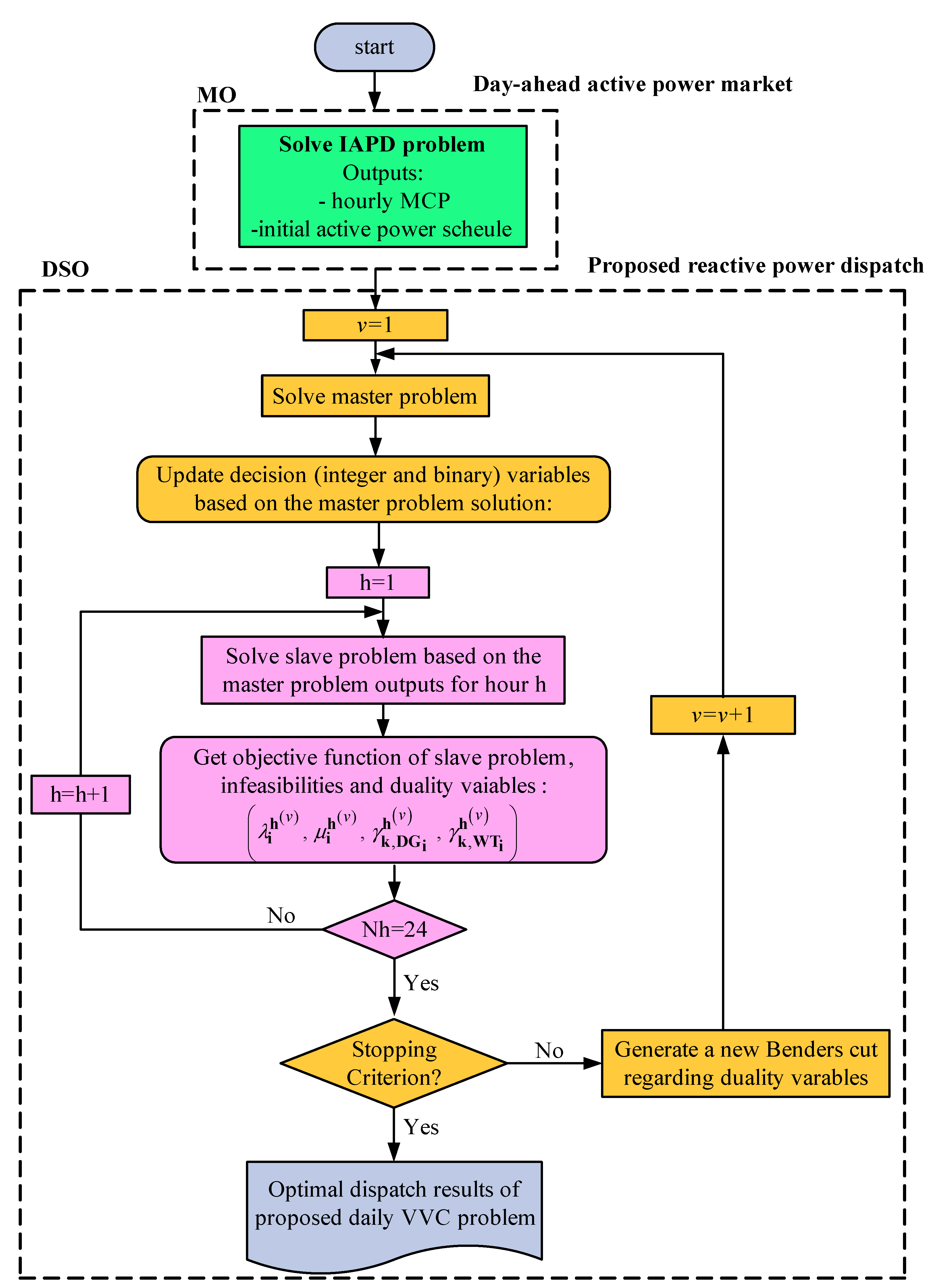
5. Benders Decomposition Algorithm

The proposed daily VVC model addressed in this paper is formulated as an MINLP problem. The complexity of solving nonlinear optimization problems with integer variables and a great number of continuous variables motivates us to implement decomposition techniques, such as the Benders decomposition algorithm. The general MINLP problem has been divided by means of the Benders decomposition algorithm into two structures, master and slave, which provides an iterative procedure between both structures in order to achieve an optimal solution [25]. The proposed solution methodology is modeled in GAMS software using the CPLEX solver for solving the Mixed Integer Programming (MIP) of the master problem and the CONOPT solver for solving the Non-Linear Programming (NLP) of the slave problem.
The Benders decomposition algorithm is described as follows:
Master Problem: The master problem decides on tap setting of OLTC, steps of Sh.Cs, and values of binary variables related to the cost of reactive power provided by DGs and WTs in order to minimize the costs of switching operations. The master problem solution is transferred to the slave problem. The objective function of master problem minimizes:
f m a s t e r = f 5 + α
Subject to the constraints Equations (46)–(50) and the Benders linear cuts as:
α f s l a v e ( m ) + h = 1 N h i = 1 N S C λ i h ( m ) ( C S t e p i h C S t e p i h ( m ) ) + h = 1 N h μ h ( m ) ( T a p h T a p h ( m ) ) + k = 0 2 h = 1 N h i = 1 N D G γ k , D G i h ( m ) ( W k , D G i h W k , D G i h ( m ) ) + k = 0 2 h = 1 N h i = 1 N W T γ k , W T i h ( m ) ( W k , W T i h W k , W T i h ( m ) )   m = 1 , 2 ,   , v 1
where v is the iteration counter. The only real variable α in Equations (51) and (52), which contain the infeasibility costs, is an underestimation of the slave problem costs. The Benders linear cuts, which are updated for every iteration, join the master and slave problems. An additional cut is added to the master problem at each iteration with information about the objective value of slave problem in the previous iteration and the dual variables associated with the decision variables fixed by the master problem in the previous iteration. This information helps the master problem to make a new decision and reach the optimal solution.
Because of the absolute (ABS) function included in the master problem, this model expresses a NLP model with discontinuous derivatives (DNLP). The only reliable way to solve a DNLP model is to reformulate it as an equivalent smooth model. The standard reformulation approach for the ABS function is to replace the ABS function with the auxiliary positive variables, g + and  g , as follows:
| g ( X ) | = g + +  g
providing that:
g ( X ) = g +  g
Therefore, the discontinuous derivative from the ABS function has disappeared and the part of the model shown here is smooth. So, the master problem is formulated as a MIP problem.
Slave problem: The slave problem formulation is nearly similar to the main problem in that all the integer variables are fixed to given the value obtained by the master problem. However, there could be some cases where the master problem’s solution makes the NLP slave problem infeasible. To avoid these cases at each iteration, artificial variables are added to some constraints and embedded in the objective function so that the objective function minimizes the technical infeasibilities of operation [26]. Therefore, the slave problem not only verifies the technical feasibility of the master problem solution but also gives the optimal dispatches of generation units. At the last iteration, the final solution of the problem has to be feasible and optimal, that is all of these artificial variables should be equal to zero. The slave problem is formulated below:
f s l a v e = f 1 + f 2 + f 3 + f 4 + M h = 1 N h i L ( u i h + w )
It is subject to the constraints of Equations (42)–(45) as well as the following constraints:
P G , i h P D , i h = | V i h | j = 1 N B u s | V j h | | Y i j | c o s ( θ i h θ j h φ i j ) ( Q G , i h + q i h ) Q D , i h = | V i h | j = 1 N B u s | V j h | | Y i j | sin ( θ i h θ j h φ i j )
q i h = { u i h w i L 0 o t h e r w i s e
C S t e p i h = C S t e p i h ( v )   :   λ i h ( v )
T a p h = T a p h ( v )   :   μ h ( v )
W k , D G i h = W k , D G i h ( v )   :   γ k , D G i h ( v )
W k , W T i h = W k , W T i h ( v )   :   γ k , W T i h ( v )
where u i h and w are the positive artificial variables of optimization problem and M is a large enough positive constant. The constraints of Equations (58)–(61) demonstrate the dual variables (sensitivities) associated with the discrete variables specified previously by the master problem. These dual variables and the objective value computed by the slave problem are applied to create new Benders cuts for the subsequent iteration.
Figure 3. Flowchart of the optimization problem based on the Benders decomposition algorithm.
Applsci 05 01284 g003

Stopping Criterion

The Benders decomposition algorithm ends when (a) the solution created by the master problem is feasible; and (b) the slave problem costs computed through the slave problem (upper bound) and the variable α (lower bound) computed through the master problem are close enough.
The procedure of the Benders decomposition algorithm for the proposed two stage model of daily VVC is shown in Figure 3.
According to the flowchart of the Benders decomposition algorithm, the following steps are implemented:
Step 1: Initialization. Initialize the iteration counter, ν = 1. Solve the initial MIP master problem with objective function Equation (51) and subject to Equations (46)–(50). Its solution provides C S t e p i h ( v ) , T a p h ( v ) , W k , D G i h ( v ) , W k , W T i h ( v ) , and α ( v ) . In this step, Equation (52) is not considered for initialization.
Step 2: Slave problem solution. Solve the NLP slave problem for all hours. The solution of this problem is the optimal dispatches of generation units, i.e. Q D G , i h , Q W T , i h , Q D i s c o h , Δ P D i s c o L , h , Δ P D G , i L , h , Δ P W T , i L , h , Δ P D i s c o A d j , h , Δ P D G , i A d j , h , and Δ P W T , i A d j , h , with dual variable values λ i h ( v ) , μ h ( v ) , γ k , D G i h ( v ) , and γ k , W T i h ( v ) .
Step 3: Convergence checking. If the convergence criterion is satisfied, the optimal solution is the last values attained for variables. Otherwise, the algorithm continues with the next step.
Step 4: Master problem solution. Update the iteration counter, ν = v + 1. Solve the MIP master problem with objective function Equation (51) and subject to Equations (46)–(50) and (52).
The algorithm continues with Step 2.

6. Simulation Results

The 22 bus 20-kV radial distribution test system [
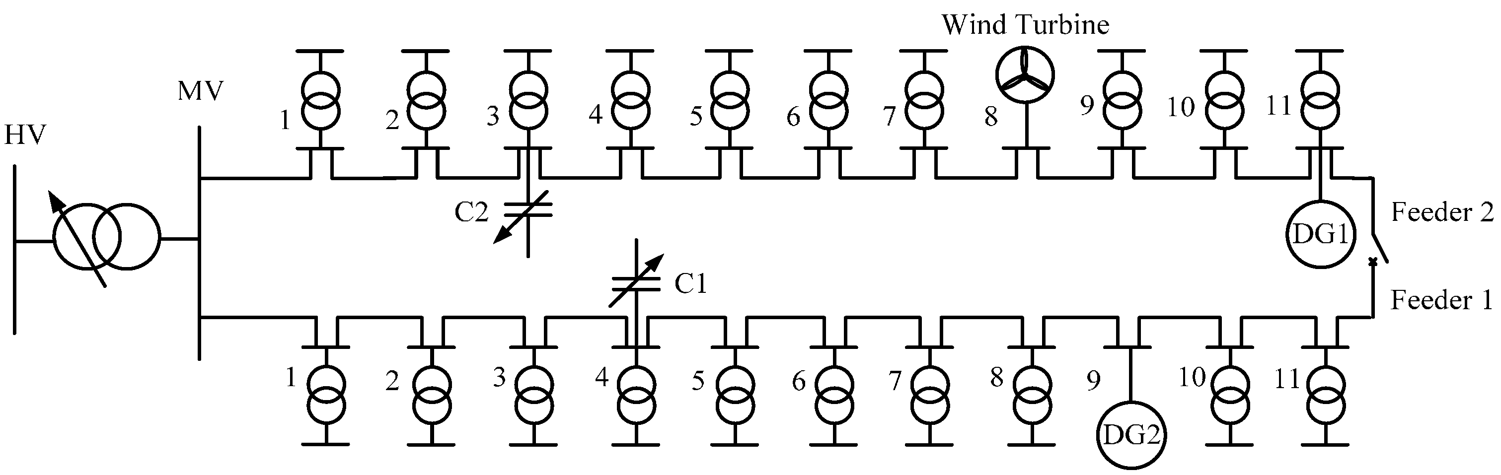
17] is modified and used for this study. The single line diagram of the test distribution network is shown in Figure 4. The system data are given in the Appendix. The HV/MV tap changing transformer has 11 tap positions and each tap ratio is 0.01 p.u. The maximum permissible daily number of operations of the transformer is 20. Voltage limits are considered to be ±5% of nominal voltage. The capacitor banks 1 and 2 have the capacity of 1000 kVAr with five switching steps of 200 kVAr. Three DERs including two DGs and a WT are connected at the distribution buses, as shown in Figure 4. General parameters such as the capacity, location, and CO2 emissions of generation units have been reported in Table 1. The values of C O 2 , c a p and E P C C O 2 are assumed to be 0.1 (ton/MWh) and 40 ($/ton), respectively [27].
Figure 4. The single line diagram of a 22-bus distribution test system.
Applsci 05 01284 g004
Table 1. Capacity, location, and emissions of generation units.
neration UnitCapacityLocationCO2 (ton/MWh)
Disco20 MVA-0.927
DG1400 kWBus 11 in feeder 20.489
DG21000 kWBus 9 in feeder 10.724
WT500 kWBus 8 in feeder 10
Table 2 shows the generation unit selling bids, including the blocks of bid power and the generation bid prices.
Table 2. Selling bids offered by generation units.
Generation UnitHourBlock NumberQuantity (kW)Price ($/kWh)
DG11–2412000.045
21000.05
31000.06
DG21–2414000.042
24000.05
32000.06
WT1–611000.041
7–1013660.041
11–1514420.041
16–1815000.041
19–2214800.041
23–2411000.041
Disco 1–8180000.04
9–10180000.045
11–13180000.05
14–15180000.052
16180000.053
17180000.054
18–19180000.053
20–22180000.052
23–24180000.05

6.1. Active Power Market Schedule Obtained by the MO

The linear programming of IAPD is programmed in the GAMS and solved by the solver CPLEX. The output of this program provides the hourly MCP and the accepted bid power of each generation unit for the next day, as indicated in Table 3. The schedule of each generation unit is sent to the DSO for verifying technical validation.

6.2. Daily Optimal Dispatches of VVC Devices
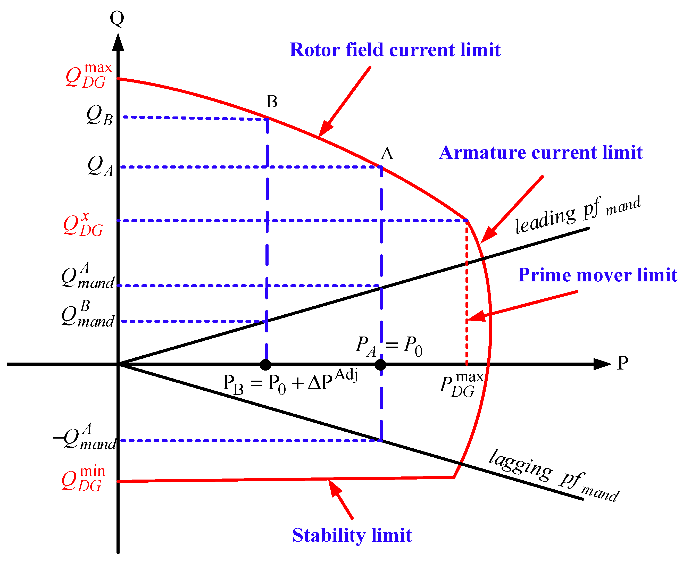
Table 4 and Table 5 present the data of DERs, including information characterizing the capability diagrams of the generator, components of offered prices of reactive power, the generator adjustment price, and the maximum admitted change as a percentage of its IAPD. The cost of reactive power generated by Disco, corresponding adjustment price, and maximum admitted change in its IAPD are 0.022 ($/kVArh), 0.09 ($/kWh), and 40%, respectively. The mandatory power factor ( p f m a n d   
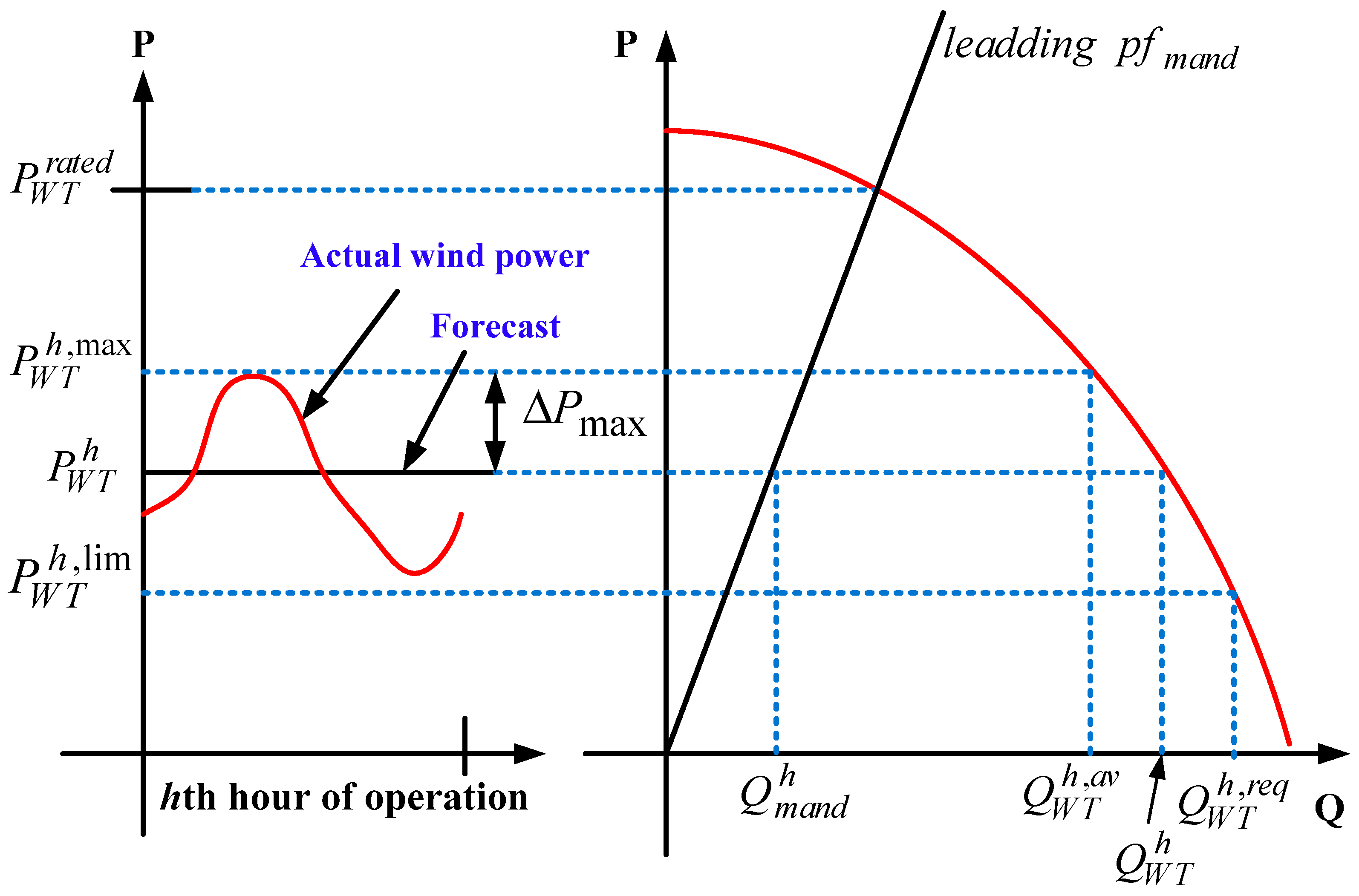
) has been taken to be 0.95. The maximum variability of the actual hourly wind power from the forecasted value is considered to be 10% of the forecasted value.
Table 3. Initial active power schedule.
Hour P D i s c o i n i (kW) P D G 1 i n i (kW) P D G 2 i n i (kW) P W T i n i (kW) M C P ($/kWh)Hour P D i s c o i n i (kW) P D G 1 i n i (kW) P D G 2 i n i (kW) P W T i n i (kW) M C P ($/kWh)
1422.623004001000.05134264.64008004420.06
276.123004001000.05142056.340010004420.06
3468.893004001000.0515260.6640010004420.06
4626.393004001000.0516187.8940010005000.06
5659.853004001000.05172008.140010005000.06
6691.353004001000.05185069.7640010005000.06
7488.353004003660.0519589740010004800.06
8801.393004003660.05205756.2340010004800.06
91375.44008003660.06214646.840010004800.06
104003.94008003660.06222925.0140010004800.06
114651.494008004420.0623598.894008001000.06
124758.84008004420.062480.124008001000.06
Table 4. Characteristics of the DGs.
R P D G m a x (kW) Q D G m a x (kVAr) Q D G m i n (kVAr)   Q D G x (kVAr) ρ 0   ($) ρ 1 ($/MVArh) ρ 2 ($/MVArh) ρ A d j ($/kWh) x m a x
DG1400400−4004000.623230.0850%
DG210001000−6008000.830300.07550%
Table 5. Characteristics of the WT.
DER V c , m a x (p.u.)   I c , m a x (p.u.)X (p.u.) Q W T m i n (kVAr) a 0   ($) ρ A d j ($/kWh) a l b l x m a x
WT1.41.240.2−2500.90.09510.140.00350%
In order to calculate the depreciation cost of OLTC, the installation cost of an OLTC is assumed to be $ 400 , 000 ( = 20 , 000 / MVA × 20   MVA ) , as reported in [26]. The total number of acceptable switching operations of each OLTC can be 143,080 times (=20 steps/day × 365 days/year × 20 years × 0.98 availability factor). Thus, the depreciation cost for each step change ( D T a p ) is $2.79. Also, the installation cost for each Sh.C is $11,600 ( = 11 , 600 / MVA × 1   MVA ) as given in [26]. Each Sh.C can be operated 71,540 times (=10 switching operations/day × 365 days/year × 20 years × 0.98 availability factor). Therefore, the depreciation cost for each switching operation of Sh.C ( D S )   is equal to $0.162.
The daily VVC problem proposed in this paper will be tested on three different cases, as follows:

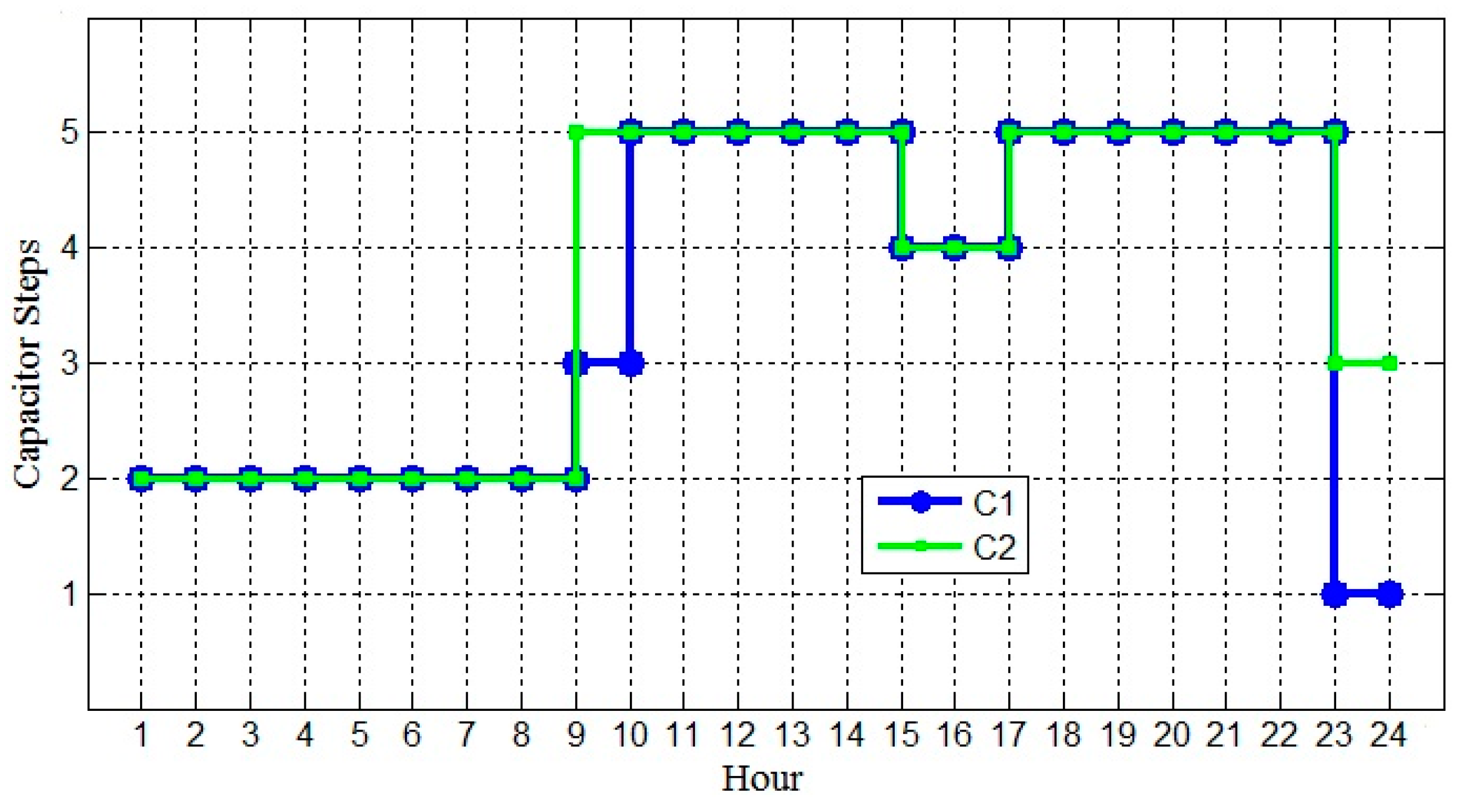
6.2.1. Case 1 (Base Case) and Implementing the Benders Decomposition Algorithm

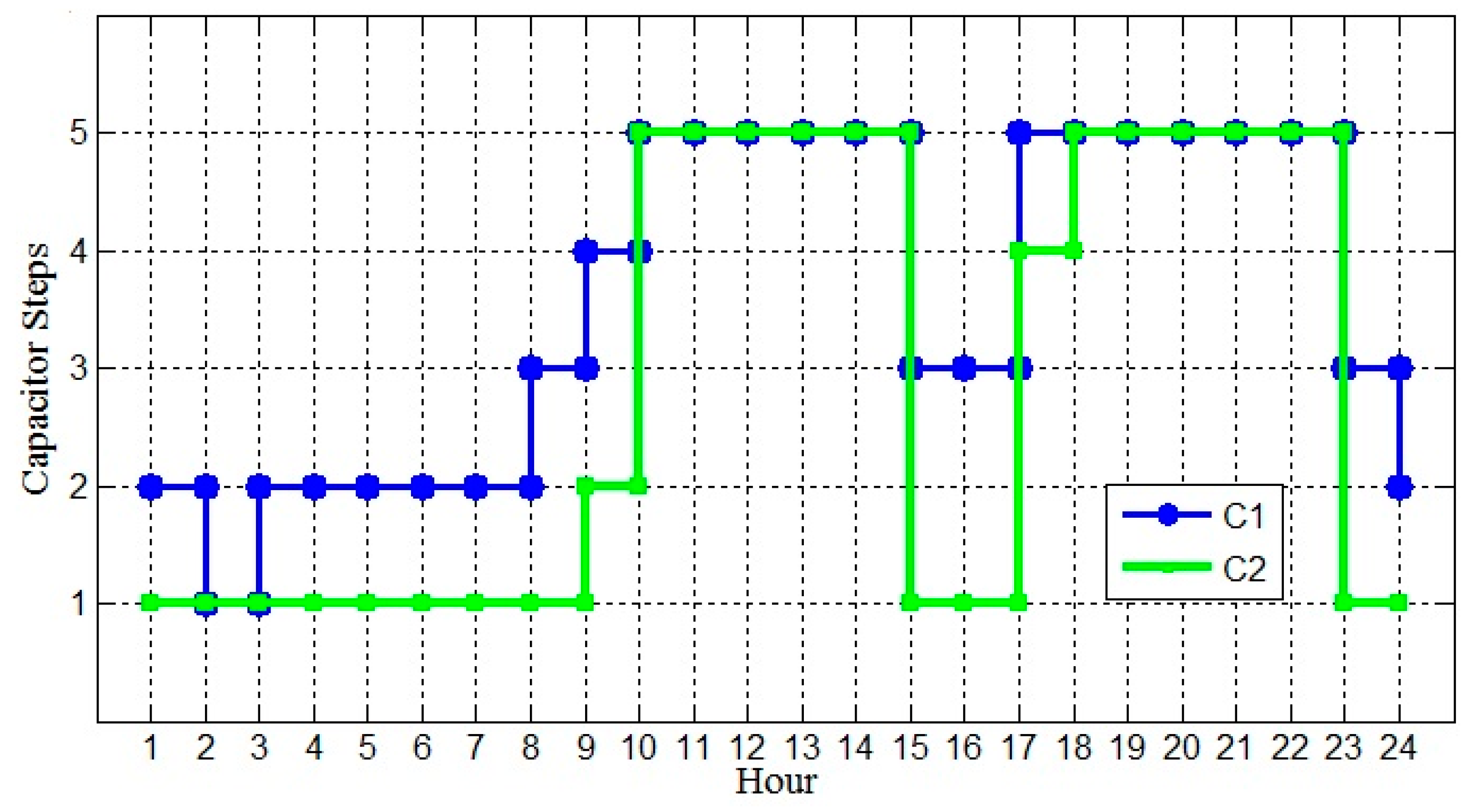
By implementing the Benders decomposition algorithm, Figure 5 shows the hourly optimal dispatch results of the Sh.Cs for case 1. The number of switching operations for C1 and C2 is 9 and 7, respectively, which is less than the maximum allowable daily number of operations (10). Moreover, because of the high depreciation cost of OLTC, the tap position of OLTC is fixed at 1.04 pu during the whole day. 
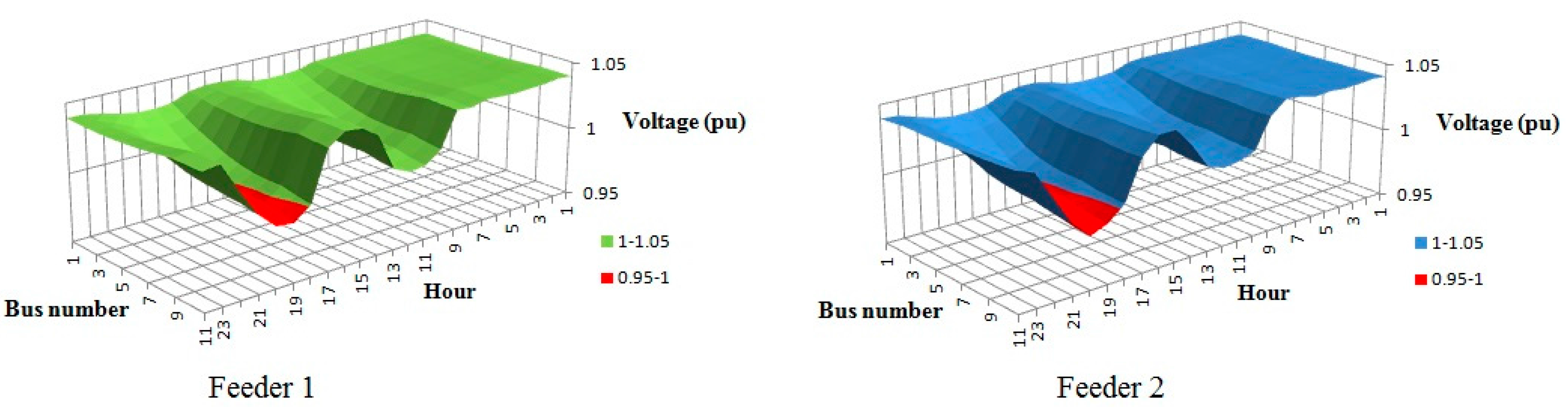
Table 6 shows the optimal dispatch of generation units. In this case, the change in the IAPD corresponding to operation or security enforcements is not necessary. So, all Δ P A d j variables are zero. Regarding the Δ P L variables, these variables are zero for DG1 and WT for all hours. Hence, the power losses of network are balanced in the two buses using Disco and DG2. The voltage profiles at the buses of feeders 1 and 2 are illustrated in Figure 6. In this figure, the voltages of buses are brought back to the acceptable range of 0.95 to 1.05 pu for 24 h.
Figure 5. Daily optimal dispatches of the Sh.Cs for case 1.
Applsci 05 01284 g005
Figure 6. Voltage profile of feeders 1 and 2 after Volt/Var control for case 1.
Applsci 05 01284 g006

6.2.2. Case 2: Considering Functions f 1 , f 2 , f 3  and f 4 . and Implementing the DICOPT Solver

In order to validate the results obtained by the proposed approach, the same problem has been tested by relaxing all constraints of the daily number of switching operations. In this case, since the optimal dispatch results of OLTC and Sh.Cs for each hour are not correlated with the solutions of the other hours, the daily VVC problem can be solved separately for each hour using the DICOPT solver. The daily optimal dispatch results of OLTC and Sh.Cs corresponding to the objectives of f 1 to f 4 are illustrated in Figure 7 and Figure 8, respectively. As seen in Figure 8, the number of operations of C1 and C2 are 12 and 16, respectively, which is higher than the acceptable maximum. Table 7 provides the optimal reactive power dispatch of generation units in case 2. In order to confirm the effectiveness of the proposed method based on the Benders decomposition algorithm, Table 8 provides a comparison between the results of cases 1 and 2. From the comparison of results shown in Table 8, it has been observed that despite the limited switching operations included in the Benders decomposition-based proposed method, the total cost decreases to $449.26, compared to $477.761 when no restriction is imposed on the switched devices; this confirms the effectiveness of Benders decomposition. On the other hand, when the limitation on switching operations of control devices is not considered, the active power loss has decreased from 998.134 kW to 954.506 kW. This is due to the fact that an unlimited number of switching operations provides a more flexible control of the power flow to regulate the voltage within its admissible range and to fulfill the operational constraints.
Table 6. Daily optimal dispatch of generation units for case 1.
HourDiscoDG1DG2WT
Δ P L (kW) Δ P A d j (kW)Q (kVAr) Δ P L (kW) Δ P A d j (kW)Q (kVAr) Δ P L (kW) Δ P A d j   (kW)Q (kVAr) Δ P L (kW) Δ P A d j   (kW)Q (kVAr)
12.31000052.6400−23.8200−32.87
22.930000−53.8900−131.4800−32.87
32.30000098.6100−35.1000−32.87
42.880000−35.5800131.480032.87
50000059.912.72044.530032.87
63.070000−7.2100131.480032.87
70000012.603.77063.9100120.30
80000098.614.380132.9200171.89
910.510000−30.4000262.9600120.30
10001043.7600131.4863.380283.7900471.50
11001432.1800395.4289.310292.3200384.72
12001515.2600400.0094.750294.1000384.72
13001223.600313.0373.410287.0900384.72
1417.010000131.4800265.0700275.70
1512.310000131.4800−223.8500−145.29
1612.990000131.4800−219.350
1716.990000131.4800328.7000157.86
18111.5001854.3200400.0000328.7000366.61
19161.9002472.0300400.0000328.7000366.61
20162.8402648.1300131.4800328.7000366.61
2199.9501850.0400131.4800328.7000366.61
2233.500560.7700131.4800328.7000366.61
2300000131.486.500265.100028.26
246.940000−28.980093.810032.87
Figure 7. Daily optimal tap positions of OLTC for case 2.
Applsci 05 01284 g007
Figure 8. Daily optimal dispatches of the Sh.Cs for case 2.
Applsci 05 01284 g008
Table 7. Daily optimal reactive power dispatches of generation units for case 2.
HourDisco (kVar)DG1 (kVar)DG2 (kVar)WT (kVar)HourDisco (kVar)DG1 (kVar)DG2 (kVar)WT (kVar)
1087.8641.0266.65131228.46307.42286.66384.72
2065.1677.6237.94140131.48264.96275.53
3093.5357.3479.36150131.48112.66115.30
4098.61105.25124.29160131.48166.54246.82
5098.57110.98127.49170131.48318.69366.61
6098.61120.54137.52181852.32400328.70366.61
7098.61132.63165.34192469.08400328.70366.61
8098.6195.55209.17202368.11400328.70366.61
90131.48190.22229.27211848.24131.48328.71366.61
101013.82160.49283.26471.5022560.19131.48328.70366.61
111436.91389.77291.78384.72230131.48109.34183.21
121514.24400.00293.51384.72240131.48235.04130.39
Table 8. Comparison of optimal results in cases 1 and 2.
Different Parts of Objective FunctionCase 1Case 2
Benders DecompositionDICOPT Solver
Number of switching operations of OLTC04
Number of switching operations of C1912
Number of switching operations of C2716
Total active power losses (kWh)998.134954.506
Depreciation cost of OLTC ($)011.16
Depreciation cost of Sh.Cs ($)2.5924.536
Total cost of active power losses ($)59.6457.07
Total cost of reactive power ($)387.03404.995
Total cost ($)449.26477.761

6.2.3. Case 3: Stressed Operation for Peak Hours and Implementing the Benders Decomposition Algorithm

In this case, due to the operational issues, the maximum reactive power of Disco was limited to peak hours (18–21) to get a more stressed operation situation. The maximum reactive power of Disco was decreased by 1300 kVAr, 1920 kVAr, 1860 kVAr, and 1050 kVAr at hours 18, 19, 20, and 21, respectively. Table 9 presents the results obtained for reactive power dispatches of generation units for peak hours. As indicated in Table 9, the Δ P A d j variable is not zero for Disco and DG2. Also, the reactive power of DG1 is increased by 400 kVar (maximum reactive power capability) at hours 20 and 21. Furthermore, since the active and reactive power values are coupled via the capability diagram, a reduction in the active power generation of DG2 takes place to adjust for the reactive power requirements of the system. The other results of daily optimal dispatches of generation units, OLTC, and Sh.Cs are not changed. Concerning the objective function, its final value is $714.99. This value is much greater than that of case 1 because it comprises the adjustment costs of the initially scheduled active powers.
Table 9. Daily optimal reactive power dispatches of generation units for peak hours for case 3.
HourDiscoDG1DG2WT
Δ P L (kW) Δ P A d j   (kW)Q (kVar) Δ P L (kW) Δ P A d j (kW)Q (kVar) Δ P L (kW) Δ P A d j   (kW)Q (kVar) Δ P L (kW) Δ P A d j   (kW)Q (kVar)
18125.73478.791300004000−478.79895.7600366.61
19174.714461.011920004000−461.01892.2000366.61
20147.39172.381860004000−172.38834.4800366.61
2196.68286.481050004000−286.48857.300366.61

7. Conclusions

This paper presented a new approach based on the energy market and reactive power dispatch considering the reactive power cost of DERs in VVC in distribution networks. For this purpose, a new pricing framework was presented to determine the cost of reactive power produced by DERs including synchronous machine-based DGs and WTs. In the proposed method, the initial scheduled active powers of Disco and DERs were determined in the day-ahead active power market. Then, the results were surrendered to the DSO, who performed daily VVC testing based on the proposed active power dispatch in order to determine the optimal dispatches of VVC devices. Due to the coupling between active and reactive power of DERs, in the proposed model, this issue was addressed by considering the capability diagram of DERs defined in the PQ plane. A Benders decomposition technique was applied to cope with the complexity of solving the daily VVC problem as a MINLP problem. It was concluded from the research results that incorporating the cost of reactive power support of generation units in the developed model would encourage the DERs to actively contribute to the reactive power support as an ancillary service.

Author Contributions

All authors discussed and agreed on the main idea and scientific contribution. Abouzar Samimi did mathematical modeling in the anuscript. Also, Abouzar Samimi performed simulations and wrote simulation sections. Abouzar Samimi and Ahad Kazemi contributed in manuscript writing and revisions.

Conflicts of Interest

The authors declare no conflict of interest.

Nomenclature

N W T / N D G total number of WTs/DGs
N h total number of hours
N B u s number of buses
L set of buses which has DER or Sh.C
P D G , i h / P W T , i h / P D i s c o h generated active power by the ith DG/ith WT/Disco at the hth hour
π D G , i h / π W T , i h / π D i s c o h price of the electrical energy generated by the ith DG/ith WT/Disco for the hth hour
C O 2 , D i s c o CO2 emissions related to Disco (ton/MW)
C O 2 , D G , i   /   C O 2 , W T , i CO2 emissions from the ith DG/ith WT (ton/MW)
C O 2 , c a p allowable CO2 emissions (ton/MW)
E P C C O 2 CO2 emissions penalty cost ($/ton)
M C P h market clearing price at the hth hour
P B i d D i s c o h / P B i d D G , i h / P B i d W T , i h maximum generation bid quantity offered by Disco/ith DG/ith WT at the hth hour
P W T r a t e d rated active power of WT
T a p h tap position of OLTC at hth hour
C S t e p i h step position of ith Sh.C at hth hour
D T a p depreciation cost for each step change of OLTC
D S depreciation cost for each switching operation of Sh.C
T a p m i n ( T a p max ) minimum (maximum) tap position of OLTC
C S t e p i m i n ( C S t e p i m a x ) minimum (maximum) step of ith Sh.C
N O L T C m a x maximum permissible daily number of operations of OLTC
N S h . C ,   i m a x maximum permissible daily number of switching operations of ith Sh.C
P G , i h ( P D , i h ) generated (consumed) active power at bus i at hour h
Q G , i h ( Q D , i h ) generated (consumed) reactive power at bus i at hour h
V i h voltage of bus i at hour h
Δ P D i s c o L , h /   Δ P D G , i L , h   / Δ P W T , i L , h amount of increasing generation corresponding to the contribution of Disco/ith DG/ith WT to balance losses at hth hour
P D i s c o i n i , h /   P D G , i i n i , h / P W T , i i n i , h initially active power of Disco/ith DG/ith WT scheduled by the Market Operator at hth hour
Δ P D i s c o A d j , h /   Δ P D G , i A d j , h / Δ P W T , i A d j , h amount of generation adjustment of Disco/ith DG/ith WT at hth hour due to enforcement of operation constraints
x D i s c o m a x / x D G , i m a x / x W T , i m a x maximum change regarding the initial active power admitted by Disco/ith DG/ith WT
ρ A d j D i s c o h / ρ A d j D G , i h / ρ A d j W T , i h adjustment price offered by Disco/ith DG/ith WT at hth hour
Q D i s c o   h / Q D G , i h / Q W T , i h generated reactive power by Disco/ith DG/ith WT at hth hour
W k , D G i h / W k , W T i h binary variable corresponding to the cost of reactive power of ith DG/ith WT at hth hour
I c ( V c ) converter’s current (voltage) of WT
V g voltage at the grid connection point for WT
C L C cost of losses component
L O C lost opportunity cost
λ i h / μ h dual variable of C S t e p i h / T a p h
γ k , D G i h , γ k , W T i h dual variables of W k , D G i h and W k , W T i h defined previously by the master problem, respectively

Appendix: Data of 22 Bus 20-kV Radial Distribution Test System

The Line data and the load characteristics are listed in Table A1 and Table A2, respectively. Also, the load profiles in the 24 h are illustrated in Figure A1.
Table A1. Line data for the test network.
Feeder 1Feeder 2
NameFromToLength (km)R (ohm/km)X (ohm/km)NameFromToLength (km)R (ohm/km)X (ohm/km)
L1-1Substation15.70.16670.1491L2-1Substation14.90.19390.1735
L1-2122.30.4130.3696L2-2123.30.28790.2576
L1-3232.30.4130.3696L2-3232.430.39090.3498
L1-4341.640.57930.5183L2-4341.260.7540.6746
L1-5451.90.50.4474L2-5451.790.53070.4749
L1-6561.840.51630.462L2-6562.90.32760.2931
L1-7672.040.46570.4167L2-7673.240.29320.2623
L1-8782.120.44810.4009L2-8782.30.4130.3696
L1-9893.70.25680.2297L2-9892.60.36540.3269
L11-109103.10.30650.2742L2-109102.50.380.34
L11-1110110.851.11761L2-1110110.581.63791.4655
Table A2. The load characteristics in each feeder.
Feeder 1Feeder 2
Bus NumberMaximum Active Power (kW)Type of CustomerPower FactorBus NumberMaximum Active Power (kW)Type of CustomerPower Factor
118210.8156020.85
228010.8228010.8
338520.85335010.8
456020.85463010.8
542020.85556010.8
638510.8638520.85
731520.85728010.8
835010.880--
90--924520.85
1028010.81028020.85
1149010.81156010.8
Type 1: Commercial; Type 2: Residential.
Figure A1. The load profile of commercial and residential loads over the 24 h.
Applsci 05 01284 g009

References

  1. Park, J.Y.; Nam, S.R.; Park, J.K. Control of a ULTC considering the dispatch schedule of capacitors in a distribution system. IEEE Trans. Power Syst. 2007, 22, 755–761. [Google Scholar] [CrossRef]
  2. Liang, R.H.; Wang, Y.S. Fuzzy-based reactive power and voltage control in a distribution system. IEEE Trans. Power Deliv. 2003, 18, 610–618. [Google Scholar] [CrossRef]
  3. Liu, M.B.; Canizares, C.A.; Huang, W. Reactive power and voltage control in distribution systems with limited switching operations. IEEE Trans. Power Syst. 2009, 24, 889–899. [Google Scholar] [CrossRef]
  4. O’Donnel, J. Voltage Management of Networks with Distributed Generation. Ph.D. Dissertation, School of Engineering and Electronic, University of Edinburgh, Edinburgh, UK, September 2007. [Google Scholar]
  5. Niknam, T. A new approach based on ant colony optimization for daily Volt/Var control in distribution networks considering distributed generators. Energy Convers. Manag. 2008, 49, 3417–3424. [Google Scholar] [CrossRef]
  6. Niknam, T.; Firouzi, B.; Ostadi, A. A new fuzzy adaptive particle swarm optimization for daily Volt/Var control in distribution networks considering distributed generators. Appl. Energy 2010, 87, 1919–1928. [Google Scholar] [CrossRef]
  7. Niknam, T. A new HBMO algorithm for multiobjective daily Volt/Var control in distribution systems considering distributed generators. Appl. Energy 2011, 88, 778–788. [Google Scholar] [CrossRef]
  8. Niknam, T.; Zeinoddini Meymand, H.; Doagou Mojarrad, H. A novel Multi-objective Fuzzy Adaptive Chaotic PSO algorithm for Optimal Operation Management of distribution network with regard to fuel cell power plants. Eur. Trans. Electr. Power 2011, 21, 1954–1983. [Google Scholar] [CrossRef]
  9. Madureira, A.G.; Pecas Lopes, J.A. Coordinated voltage support in distribution networks with distributed generation and microgrids. IET Renew. Power Gener. 2009, 3, 439–454. [Google Scholar] [CrossRef]
  10. Azimi, R.; Esmaeili, S. Multiobjective daily Volt/VAr control in distribution systems with distributed generation using binary ant colony optimization. Turkish J. Electr. Eng. Comput. Sci. 2013, 21, 613–629. [Google Scholar]
  11. Zare, M.; Niknam, T. A new multi-objective for environmental and economic management of Volt/Var Control considering renewable energy resources. Energy 2013, 55, 236–252. [Google Scholar] [CrossRef]
  12. Malekpour, A.R.; Tabatabaei, S.; Niknam, T. Probabilistic approach to multi-objective Volt/Var control of distribution system considering hybrid fuel cell and wind energy sources using Improved Shuffled Frog Leaping Algorithm. Renew. Energy 2012, 39, 228–240. [Google Scholar] [CrossRef]
  13. Zare, M.; Niknam, T.; Abarghooee, R.A.; Amiri, B. Multi-objective probabilistic reactive power and voltage control with wind site correlations. Energy 2014, 66, 810–822. [Google Scholar] [CrossRef]
  14. Meegahapola, L.; Fox, B.; Littler, T.; Flynn, D. Multi-objective reactive power support from wind farms for network performance enhancement. Int. Trans. Electr. Energy Syst. 2013, 23, 135–150. [Google Scholar] [CrossRef]
  15. Viawan, F.; Karlsson, D. Combined local and remote voltage and reactive power control in the presence of induction machine distributed generation. IEEE Trans. Power Syst. 2007, 22, 2003–2012. [Google Scholar] [CrossRef]
  16. Elkhatib, M.E.; Shatshat, R.E.; Salama, M.M.A. Decentralized Reactive Power Control for Advanced Distribution Automation Systems. IEEE Trans. Smart Grid 2012, 3, 1482–1490. [Google Scholar] [CrossRef]
  17. Homaee, O.; Zakariazadeh, A.; Jadid, S. Real-time voltage control algorithm with switched capacitors in smart distribution system in presence of renewable generations. Int. J. Electr. Power Energy Syst. 2014, 54, 187–197. [Google Scholar] [CrossRef]
  18. Zakariazadeh, A.; Homaee, O.; Jadid, S.; Siano, P. A new approach for real time voltage control using demand response in an automated distribution system. Appl. Energy 2014, 117, 157–166. [Google Scholar] [CrossRef]
  19. Saraswat, A.; Saini, A.; Saxena, A.K. A novel multi-zone reactive power market settlement model: A pareto-optimization approach. Energy 2013, 51, 85–100. [Google Scholar] [CrossRef]
  20. Gomes, M.H.; Saraiva, J.T. Allocation of reactive power support, active loss balancing and demand interruption ancillary services in MicroGrids. Electr. Power Syst. Res. 2010, 80, 1267–1276. [Google Scholar] [CrossRef]
  21. Ullah, N.R.; Bhattacharya, K.; Thiringer, T. Wind Farms as Reactive Power Ancillary Service Providers—Technical and Economic Issues. IEEE Trans. Energy Convers. 2009, 24, 661–672. [Google Scholar] [CrossRef]
  22. Abarghooee, R.A.; Niknam, T.; Roosta, A.; Malekpour, A.R.; Zare, M. Probabilistic multiobjective wind-thermal economic emission dispatch based on point estimated method. Energy 2012, 37, 322–335. [Google Scholar] [CrossRef]
  23. Wong, S.; Bhattacharya, K.; Fuller, J. Long-term effects of feed-in tariffs and carbon taxes on distribution system. IEEE Trans. Power Deliv. 2010, 25, 1241–1253. [Google Scholar] [CrossRef]
  24. Lamont, J.W.; Fu, J. Cost analysis of reactive power support. IEEE Trans. Power Syst. 1999, 14, 890–898. [Google Scholar] [CrossRef]
  25. Seyyed Mahdavi, S.; Javidi, M.H. VPP decision making in power markets using Benders decomposition. Int. Trans. Electr. Energy Syst. 2014, 24, 960–975. [Google Scholar] [CrossRef]
  26. Zakariazadeh, A.; Jadid, S.; Siano, P. Economic-environmental energy and reserve scheduling of smart distribution systems: A multiobjective mathematical programming approach. Energy Convers. Manag. 2014, 78, 151–164. [Google Scholar] [CrossRef]
  27. Ghadikolaei, H.M.; Tajik, E.; Aghaei, J.; Charwand, M. Integrated day-ahead and hour-ahead operation model of discos in retail electricity markets considering DGs and CO2 emission penalty cost. Appl. Energy 2012, 95, 174–185. [Google Scholar] [CrossRef]

