Article

A Generative Model Approach for LiDAR-Based Classification and Ego Vehicle Localization Using Dynamic Bayesian Networks

1
Department of Electrical, Electronic, Telecommunications Engineering and Naval Architecture (DITEN), University of Genova, Via Opera Pia 11a, I-16145 Genoa, Italy
2
Departamento de Ingeniería de Sistemas y Automática, Universidad Carlos III de Madrid, Butarque 15, 28911 Leganés, Madrid, Spain
*
Author to whom correspondence should be addressed.
Appl. Sci. 2025, 15(9), 5181; https://doi.org/10.3390/app15095181
Submission received: 27 March 2025 / Revised: 29 April 2025 / Accepted: 3 May 2025 / Published: 7 May 2025

Abstract

:
Our work presents a robust framework for classifying static and dynamic tracks and localizing an ego vehicle in dynamic environments using LiDAR data. Our methodology leverages generative models, specifically Dynamic Bayesian Networks (DBNs), interaction dictionaries, and a Markov Jump Particle Filter (MJPF), to accurately classify objects within LiDAR point clouds and localize the ego vehicle without relying on external odometry data during testing. The classification phase effectively distinguishes between static and dynamic objects with high accuracy, achieving an F1 score of 91%. The localization phase utilizes a combined dictionary approach, integrating multiple static landmarks to improve robustness, particularly during simultaneous multi-track observations and no-observation intervals. Experimental results validate the efficacy of our proposed approach in enhancing localization accuracy and maintaining consistency in diverse scenarios

1. Introduction

Autonomous vehicles (AVs) are designed to eliminate or significantly reduce human intervention in vehicle operation, ensuring greater efficiency, safety, and autonomy in various real-world applications. The field of AV research has seen rapid advancements since the 1980s, with applications spanning transportation, agriculture, disaster response, security, and surveillance [1,2]. The ability of AVs to operate autonomously in highly dynamic and unpredictable environments relies on their ability to perceive, interpret, and adapt to their surroundings. Two fundamental paradigms govern AV research: the computationalist approach, which relies on predefined mathematical models and rigid control rules, and the cognitive approach, which allows AVs to dynamically learn and refine their internal models based on real-time sensor data [3]. While computationalist methods provide structured frameworks for decision-making, they often fail in real-world scenarios where unforeseen events and changing conditions necessitate adaptive learning and reasoning. The cognitive approach, inspired by human cognition, enables AVs to develop self-awareness, allowing them to make intelligent decisions based on past experiences and sensory inputs.
Self-awareness in AVs is a crucial capability that enables the system to comprehend its internal state while monitoring external environmental conditions. This is achieved through the integration of exteroceptive sensors (e.g., LiDAR, cameras, radar) and proprioceptive sensors (e.g., Inertial Measurement Units (IMUs), steering angle sensors, wheel speed sensors), enabling AVs to perceive both external obstacles and their own motion [4,5]. The ability to interpret and fuse data from multiple sensor sources [6,7] forms the basis of a self-aware AV, allowing it to understand its surroundings, detect anomalies, and adjust its motion accordingly.
AVs require precise and accurate perception of their surroundings to navigate safely in dynamic environments. Therefore, advanced sensors and data processing techniques are necessary to accomplish this goal [8,9]. It is also possible to significantly enhance driving performance and safety by adding additional sensors [10,11,12] that monitor physiological signals. A significant advantage of LiDAR sensors is their ability to map the environment in 3D and provide greater accuracy in distance detection and measurement compared to traditional cameras [13,14]. Nevertheless, preprocessing the dense 3D point clouds generated by LiDAR is essential for removing noise and obtaining relevant information [15]. An object’s position, velocity, count, and classification can be determined using LiDAR sensors, which provide a 3D model of the surrounding environment. Multi-Target Tracking (MTT) for AVs involves the detection and tracking of multiple objects at once. Traditionally, detection-based tracking has been used in computer vision. However, it has now been adapted for use with LiDAR data [16]. As part of MTT, LiDAR data are segmented into meaningful clusters and tracked over successive frames in order to provide AVs with an understanding of their surroundings [17].
The use of sensor fusion techniques, which integrate LiDAR and radar data, has been investigated in a variety of research areas in order to improve target perception and detection performance in AV systems [18]. The use of deep learning frameworks for classifying landmarks has been proposed as a means of optimising vehicle localization [19]. In addition, LiDAR and camera data have been integrated to improve environmental perception [20]. Multiple object detection and tracking (MODT) algorithms, which employ multiple 3D LiDARs, are used to enhance tracking accuracy by utilizing grid-based clustering techniques and advanced filtering techniques [21]. Nunes et al. [22] proposed a method for learning 3D LiDAR data based on temporal association representations. It is, however, often overlooked in these studies that the interaction between dynamic and static objects needs to be modeled. With our approach, we provide a framework that not only categorizes static and dynamic tracks, but also examines how ego vehicle clusters interact with track clusters. AVs require, indeed, interaction modeling to gain self-awareness [23] and improve their navigation and decision-making capabilities.
A key aspect of AV perception is accurately perform classification and localization of objects, which are essential for safe and efficient navigation. Classification allows AVs to distinguish between static (e.g., buildings, traffic signs, poles) and dynamic (e.g., vehicles, cyclists, pedestrians) objects. Accurate classification ensures that AVs can reliably interpret which objects remain fixed and which are moving, allowing them to anticipate interactions, make informed decisions, and optimize trajectory planning. On the other hand, localization refers to the AV’s ability to accurately determine its position and motion within an environment. Traditional localization methods, such as GPS and odometry-based approaches, often suffer from signal loss, drift, and inaccuracies in complex environments, e.g., urban canyons, tunnels, and cluttered environments. Therefore, alternative localization techniques are required to enhance reliability and robustness, particularly in dynamic environments where environmental conditions constantly change.
In this work, LiDAR-based perception is utilized to enhance both classification and localization capabilities. LiDAR generates high-resolution 3D point clouds, which allow AVs to precisely map their surroundings and distinguish between different object categories [8,9]. LiDAR’s ability to capture spatially rich depth information makes it superior to vision-based systems, particularly in adverse lighting conditions, poor weather, and complex urban environments [24]. The classification of LiDAR-based tracks into static and dynamic categories provides landmark references for localization, ensuring that AVs can estimate their position accurately even in the absence of GPS signals or external odometry updates [25]. By leveraging LiDAR-based classification techniques, AVs can use static objects as anchor points for precise localization, while simultaneously tracking and interpreting the motion of dynamic objects.
The motivation for this research extends beyond the intrinsic benefits of LiDAR sensors to its application in the pipeline used to classify and localize AVs. Navigating precisely in dynamic environments requires not only the perception of static and dynamic objects, but also their effective use for localization [26,27,28]. Using LiDAR’s capability to generate 3D point clouds, we have proposed a classification method that identifies static and dynamic tracks in the ego vehicle environment [29]. Static tracks provide reliable landmarks for ego vehicle localization because they remain invariant over time. Dynamic tracks, on the other hand, pose difficulties because of their motion [30,31]. However, the ability to understand interactions with dynamic tracks is essential. Based on this duality, we focused on accurately classifying tracks during the training phase using advanced algorithms such as Joint probababilistic data association (JPDA), Growing neural gas (GNG), and interaction dictionaries. The resulting classified static tracks are then used during testing to determine the ego vehicle’s location without relying on external odometry updates, thereby ensuring robustness in real-world conditions. These concepts are explicitly integrated into a cognitive self-awareness cycle. An AV can acquire knowledge of the structure of its environment, generate dictionaries of potential interactions with a variety of static objects, and characterize the dynamics of moving objects during the offline training phase. Afterward, during the online testing phase, the AV’s pose is continuously monitored, anomalies are detected, and the system is able to adapt to unanticipated circumstances by fusing the acquired knowledge with new sensor data using probabilistic filters, specifically an MJPF. In essence, classification and localization serve as fundamental components of the broader self-awareness strategy, continuously interacting with higher-level modules.
Recent generative modeling techniques have shown strong potential in enhancing AV perception and trajectory predictions. For instance, diffusion-based models such as LiDiff [32] have demonstrated effective LiDAR-based human motion prediction in dynamic scenes. Similarly, Xu et al. [33] introduced a Bayesian ensemble graph attention network to learn spatio-temporal relationships in dense traffic for multi-agent prediction. Generative transformer models [34] have also been employed to learn interpretable latent spaces for trajectory forecasting, particularly in multi-agent environments.
In our prior work [35], we proposed a LiDAR-based ego vehicle localization approach using individually trained interaction dictionaries for each static track. While that framework demonstrated promising results in structured testing environments, it did not address scenarios involving simultaneous interactions, unobserved intervals, or the fusion of dictionaries across tracks.
Our main contributions in this paper are as follows.
  • Innovative Classification Framework: We developed a robust method to classify static and dynamic tracks using LiDAR data, leveraging a combination of probabilistic models, including DBNs and interaction dictionaries.
  • Self-Aware Localization Strategy: We introduced a novel ego vehicle localization approach that does not rely on external odometry data during testing, enhancing autonomy in dynamic environments.
  • Simultaneous Multi-Track Interaction Modeling: We proposed a combined interaction dictionary that enables simultaneous modeling of multiple track interactions and ensures continuity during missing observations.
  • Integration of Interaction Dictionaries: We designed a methodology that combines multiple static track interactions into a unified dictionary framework, ensuring robust localization even in the absence of continuous observations.
  • Hybrid Inference with MJPF: We implemented an MJPF filter that supports hybrid discrete and continuous inference for trajectory prediction.
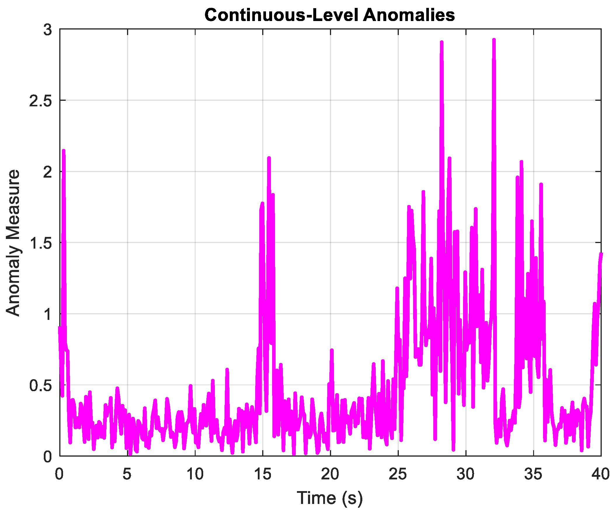
  • Generative Localization Model: We developed a generative localization model capable of statistical filtering and divergence-based anomaly detection during trajectory estimation.
  • MJPF Enhancement for Ego Vehicle Localization: We incorporated MJPF into the localization process to refine ego vehicle positioning by continuously predicting and updating its estimated trajectory based on static track interactions.
These enhancements distinguish the present work from our prior approach and contribute to a more robust data-driven localization strategy for AVs.
The remainder of this paper is organized as follows. Section 2 presents a review of the related works in LiDAR-based classification and localization. Section 3 introduces the proposed methodology, including classification, interaction dictionaries, and ego vehicle localization using MJPF. Furthermore, it details the use of combined dictionaries for improving localization accuracy and describes the DBN modeling for track classification and localization. Section 4 presents experimental results, including classification accuracy, localization performance, and anomaly detection analysis. Finally, Section 5 concludes the paper with a summary of the findings and suggests future directions.

2. Related Works

This section presents an overview of the state-of-the-art research relevant to our work, which includes multiple domains. Since our work encompasses multiple aspects, we have divided this section into two subsections. Each subsection addresses a particular aspect of our study. This approach allows for a more structured and comprehensive review of the existing literature, with special attention given to studies that make use of LiDAR data classification and ego vehicle localization in autonomous driving applications.

2.1. Classification of LiDAR Data

Recent developments in the classification of LiDAR data for autonomous driving have been focusing on enhancing object detection and semantic segmentation through the use of deep learning and sensor fusion techniques. Aksoy et al. [36] presented SalsaNet, i.e., a deep learning model developed for the efficient semantic segmentation of 3D LiDAR point clouds for autonomous driving. A bird-eye-view (BEV) projection is used to segment roads and vehicles using an encoder-decoder architecture. Moreover, they developed an automatic process for labeling LiDAR data by transfering labels from camera images to LiDAR point clouds. A multimodal 3D object detection framework based on LiDAR and camera data was developed by Zhang et al. [37]. They utilized a feature fusion network to improve detection accuracy in complex driving environments. Li et al. [38] developed a deep learning model for the classification of LiDAR point clouds, by using a convolutional neural network (CNN) to extract spatial features and enhance object recognition using LiDAR point clouds. The authors in [39] presented a lightweight semantic segmentation network optimized for embedded systems, enabling efficient inferences on hardware with constrained resources without compromising accuracy. There has been growing emphasis on integrating multi-modal data to improve the accuracy of classification. By combining LiDAR point clouds with RGB images, the FusionNet architecture enhances object recognition in complex environments by leveraging complementary information from both sources. In addition, transformer-based models have been explored for the classification of point clouds. Self-attention mechanisms are used to capture long-range dependencies within point clouds, which have been demonstrated to perform better than conventional algorithms on benchmark datasets [40]. We introduce a generative model-based technique for classifying static and dynamic tracks using LiDAR data for AV navigation that differs from existing approaches. In contrast to previous work that heavily relied on supervised learning and feature extraction, we use a combination of DBNs and interaction arrays to model the interactions between the ego vehicle and its surroundings.

2.2. Ego Vehicle Localization

AVs require accurate localization, especially in environments with limited GPS reliability. As a result of recent developments utilizing LiDAR technology, localization capabilities have been significantly enhanced: LiDAR SLAM based multi-vehicle cooperative localization using iterated split Covariance Intersection Filters (Split CIFs) is presented in [41]. Using Split CIFs with decentralized SLAM, this study enhances localization accuracy and robustness across AV networks. Based on tests performed using the CARLA simulator, their methodology demonstrates substantial improvements over traditional SLAM techniques. Persistent Homology (PH) is applied to ego-vehicle localization in [42]. PH is a topological data analysis method that is designed to extract translation and rotation invariant features from point clouds, thereby capturing their global structure without taking into consideration their local details. As a result of vectorizing these features into Persistence Images (PI), the authors are able to create fixed-size vectors from variable-size point clouds. There are three applications investigated in this paper: loop closure detection, which identifies previously visited locations based on PIs; place categorization, which effectively differentiates distinct shapes based on the global structure of point clouds; and end-to-end global localization, which integrates PIs into neural networks to improve localization accuracy. Although PIs enhance position estimation to a certain extent, they do not significantly improve orientation accuracy due to the loss of local geometric information. The study concludes that, while PH is useful for extracting global features, it is not able to capture the local geometry necessary for precise localization.
In [24], a novel method is developed to enhance vehicle localization precision in urban canyons obstructed by GPS signals by combining LiDAR with real-time kinematic positioning. With this method, the localization error can be reduced to within a few centimeters, even in densely populated areas. An innovative SLAM algorithm introduced in [43] integrates LiDAR data with inertial measurements to improve mapping accuracy in urban environments. By using this method, drift is reduced in densely populated urban areas where satellite signals are frequently obstructed. A sensor fusion technique is proposed in [44] that integrates radar and LiDAR data. It can maintain high localization accuracy even in adverse weather conditions, addressing some of the limitations of LiDAR systems, such as fog and heavy rain.
In [45], a method of precise ego-location is developed by integrating multi-view imaging with LiDAR and vectorized maps. A transformer decoder is applied in this approach, which is validated across diverse urban settings and significantly improves pose estimation over traditional approaches. Our method for ego vehicle localization differs from the aforementioned methods, as it employs a generative model based on DBNs and interaction dictionaries, leveraging pre-classified static tracks learned during training. We use an MJPF for testing, which combines continuous tracking using Kalman filters with non-linear estimation using particle filters. This approach refines the ego vehicle’s position by comparing predictions with real-time observations, allowing us to detect errors and anomalies effectively.

3. Proposed Framework

In this section, we present our proposed framework consisting of an offline training phase and an online testing phase. To ensure clarity, we have organized the discussion of each section into detailed subsections.

3.1. Offline Training Phase

Our proposed framework is depicted in Figure 1. The dataset used in our work was collected at the University of Carlos III, Madrid, using a vehicle called “iCAB” equipped with a Velodyne LiDAR Puck (VLP-16) sensor [46]. The Velodyne VLP-16 LiDAR was selected due to its widespread use in AV research and compatibility with real-time processing constraints. Despite its efficiency and 360° horizontal field of view, the sensor has limitations related to its 16-beam resolution, which may lead to lower vertical fidelity compared to more advanced LiDARs. In adverse weather conditions, such as rain or fog, signal degradation and increased noise may occur, which can affect point cloud density and downstream tracking accuracy [47]. In our work, these effects are partially mitigated through temporal filtering and clustering.
The environment has been captured using 393 frames of point cloud data. Two vehicles are included in this dataset: iCAB1 overtakes another vehicle iCAB2 at a specific point in time. In addition, the dataset contains static objects, such as buildings, trees, and poles, that are crucial for vehicle navigation and localization. Furthermore, in the offline training phase, static and dynamic tracks from the LiDAR-based dataset were classified based on previously established mathematical formulations detailed in our previous work [29]. The process involves analyzing individual tracks, extracting relevant kinematic and positional features, and applying clustering methods to segregate dynamic objects from static environmental elements.
The dataset utilized for this work includes different track sequences from the same LiDAR-based source, distinctly separate from those presented in our prior work. This ensures the robustness and generalizability of our classification approach under varying scenarios and track interactions.
It is important to remove ground points and other irrelevant data from the raw point cloud data, as part of the preprocessing step to improve the accuracy of the subsequent steps. Filtering out noise and identifying significant features in the data are also part of this process [48].

3.1.1. Detection and Tracking

For the multi-target tracking module, a finely tuned detector model is employed with precise limits on the X, Y, and Z axes, ensuring accurate placement of the bounding box. Certain parameters, including minimum segmentation distances and minimum detections per cluster, are optimized to enhance object detection. Using the joint probabalistic data association (JPDA) tracker, the thresholds for track assignment, confirmation, and deletion have been carefully defined in this module [49]. Track positions and timings are stored in a data structure, enabling detailed analysis of each object’s trajectory. Ground truth images were used to verify the tracker’s performance using the JPDA algorithm applied to LiDAR data. There have been seven distinct tracks saved, each with a unique TrackID and x and y positions. The simulator displayed bounding boxes on these tracked objects during the movement of the ego vehicle. In total, seven tracks have been selected: TrackID 14, which represents a car in front of the ego vehicle; TrackID 20, which represents a building on the right side; TrackID 1416, a static pole; TrackID 1682, a tree; TrackID 1929, a small static pole; TrackID 3159 and TrackID 3549, both representing trees. Data from odometry were used to determine the location of the ego vehicle, allowing us to analyze the trajectory in absolute coordinates. In Figure 2, the ego vehicle’s trajectory is illustrated in absolute coordinates, while Figure 3 shows the position of the seven tracks with their Track IDs relative to the ego vehicle.

3.1.2. Odometry Sensor

During the offline training phase, the odometry sensor plays a critical role in determining the position of the ego vehicle, which is necessary for localizing the ego vehicle during testing. Ego vehicle localization is enhanced by including the DBNs derived from the training phase as an additional switching variable. A critical point is that during the online testing phase, the ego vehicle localization is performed only using LiDAR data, leveraging the DBNs that have been trained with odometry sensor data.

3.1.3. Null Force Filter

The seven tracks and the trajectory of the ego vehicle are then filtered using the null force filter. In this filter, it is assumed that no external forces are affecting the motion, so the system can continue to move at its previous velocity without being affected by external forces [50]. Using this approach, we were able to obtain generalized states, including positions and velocities, for each of the seven tracks and the ego vehicle. The GNG algorithm was applied to cluster the generalized states (positions and velocities along x and y) of the ego vehicle and the tracks [51]. Using clustering, vocabularies with mean positions, mean velocities, and covariance between positions and velocities were generated. The parameters of the GNG algorithm were selected according to the size of the data points for each trajectory, ensuring that smaller trajectories have fewer nodes and larger ones have more. As mentioned above, considering the mean vectors, proposed mathematical equations have been used to create dictionaries for the classification of tracks. In Figure 4, the clustered generalized states of the seven tracks and the ego vehicle’s trajectory are shown.

3.1.4. Track Classifications

The interaction dictionary is constructed based on the mean position and velocity of each cluster, considering both the ego vehicle and tracks. Therefore, for each timestamp, a cluster index is calculated using the Euclidean distance. As part of the initialization of the interaction array, the positions of the ego vehicle, time, cluster indices, and interaction labels for both the ego vehicle and tracks are recorded.
The timing analysis was conducted for interactive clusters where both the ego vehicle and each track were simultaneously present in the space at the same time. Track 14 interacted with the ego vehicle from 1 to 14.7 s. Similarly, Track 20 had interactions with the ego vehicle from 0.7 to 14.5 s. Interactions for Track 1416 began at 15.8 s and ended at 18 s. Track 1682’s interaction took 18 to 24.8 s. Track 1929 interacted with ego vehicle from 20 to 23.4 s. The interaction time between track 3159 and ego vehicle occurs from 32.1 to 33.7 s. Finally, Track 3549 interacted with the ego vehicle between 36 and 39.3 s. Table 1 shows the initial part of the interaction array which belongs to the interactions between the ego vehicle and track 14. The track cluster index of 0 indicates that there was no interaction at that time, so the first interaction began at 1.000 s. Note that this interaction continues until the end of a particular interaction, maintaining separate interaction arrays for the ego vehicle and for each track.
The hierarchical DBN model is illustrated in Figure 5. Odometry data is used to determine the position of the ego vehicle on the left side of the DBN. There are seven different tracks on the right side, provided by the LiDAR sensor. A layer of observations is located at the bottom, where raw sensor data have been collected. The middle level of the model (i.e., a continuous level) represents our generalized states. Through the use of the GNG algorithm, the third upper layer is a discrete layer that allows us to group the generalized states into clusters. Lastly, dictionary interactions occur at the top of the DBNs, where clusters derived from GNG are considered, enabling interaction between tracked objects and the ego vehicle. A switching variable is incorporated into the DBN to distinguish static tracks from dynamic tracks according to predefined mathematical equations. As a result, these classifications play a crucial role in extending learned vocabularies during testing, particularly for localizing the ego vehicle. For this purpose, separate dictionaries are maintained for each track and ego vehicle, each containing six columns of information: time, the cluster index of the ego vehicle, the cluster index of the track, the interaction label, as well as the x and y positions of the ego vehicle. It is especially useful for predicting the position of the ego vehicle to have the interaction label, which indicates whether it is interacting with a specific track at a given time. Using these dictionaries to analyze interaction labels and spatial data, the model can more accurately predict the ego vehicle’s position relative to static tracks. This is achieved using an MJPF, which combines the strengths of Kalman filters and particle filters. Utilizing the consistent patterns in the static tracks’ data, the MJPF refines the positional estimates by comparing predictions from the DBN with real-time observations. Whenever the switching variable indicates a static state, the DBN leverages the corresponding dictionary entries to provide more accurate and robust localization of the ego vehicle. The use of this approach ensures that the localization process is both data-driven and mathematically based, greatly improving the accuracy and reliability of navigation on the ego vehicle.
During the final stage of offline training phase, we classify tracks based upon the interaction between the clustered states of the ego vehicle and the clusters of the tracks. The interaction between an ego vehicle and a dynamic track cluster should be classified as dynamic, while the interaction with a static track cluster should be classified as static. The relative velocities of the ego vehicle and the track clusters determine whether a track is static or dynamic. This is achieved by measuring the difference between the ego vehicle’s velocity and those of each track cluster over a period of time. The relative velocities are plotted in a histogram (see Section 4), and the mean plus one standard deviation ( μ + σ ) of the plotted values is used as a threshold to distinguish static and dynamic tracks. This helps to classify interactions in a robust manner, with dynamic velocities appearing above the threshold and static velocities appearing below it. This thresholding method, which is based on the mean and standard deviation, is chosen due to its statistical robustness. It not only considers the central tendency of relative velocities but also accounts for the variability in the data, enabling adaptive classification across heterogeneous environments. By setting the decision boundary dynamically, the approach becomes less sensitive to outliers and better suited to generalize across diverse driving contexts. We validated its effectiveness across two datasets, i.e., iCAB and KITTI, achieving classification accuracies of 87% and 82%, respectively, with F1 scores of 91% and 85% (see Section 4). These metrics confirm the reliability of the method across varying scenarios, including structured urban environments and dynamic traffic conditions.

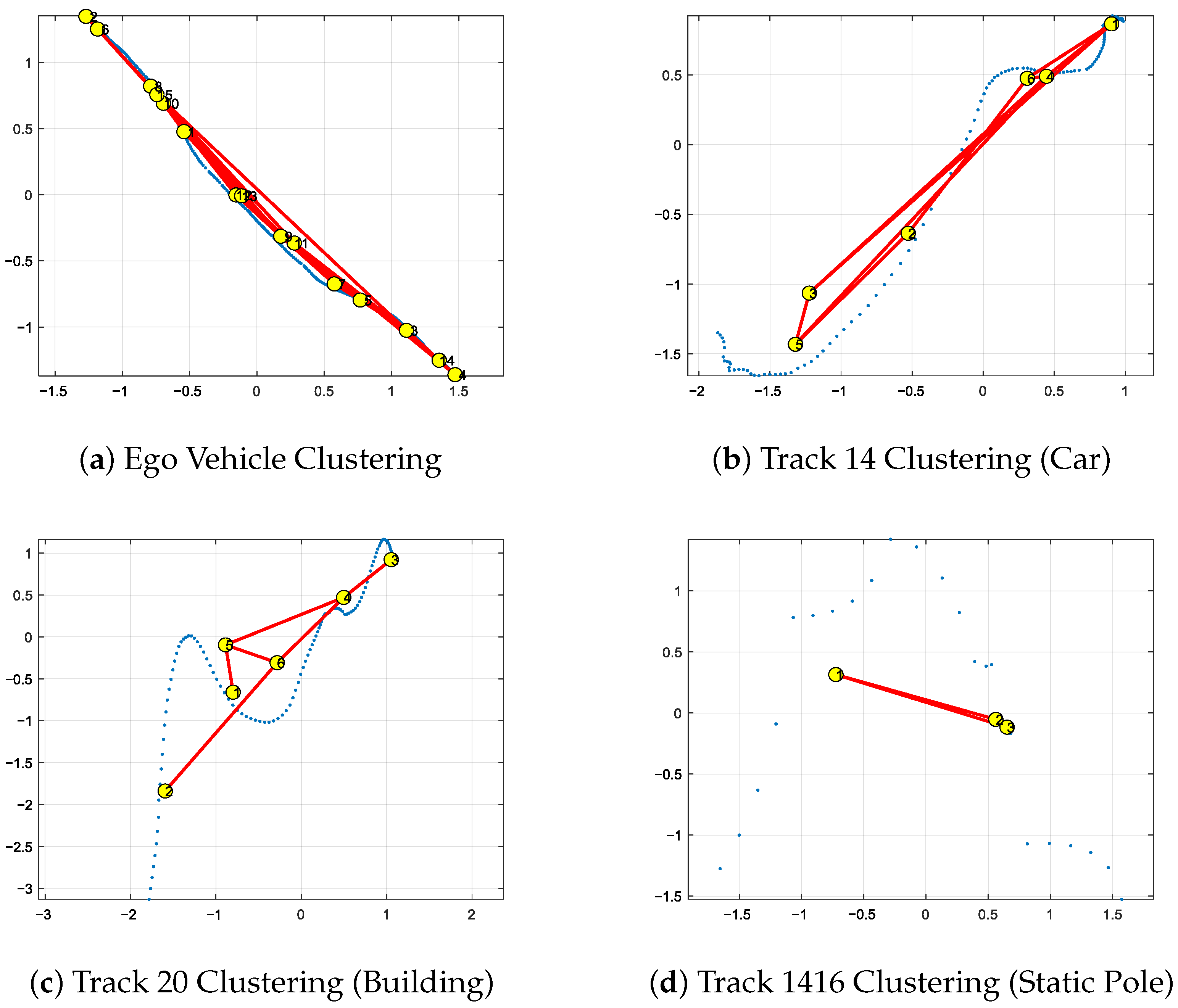
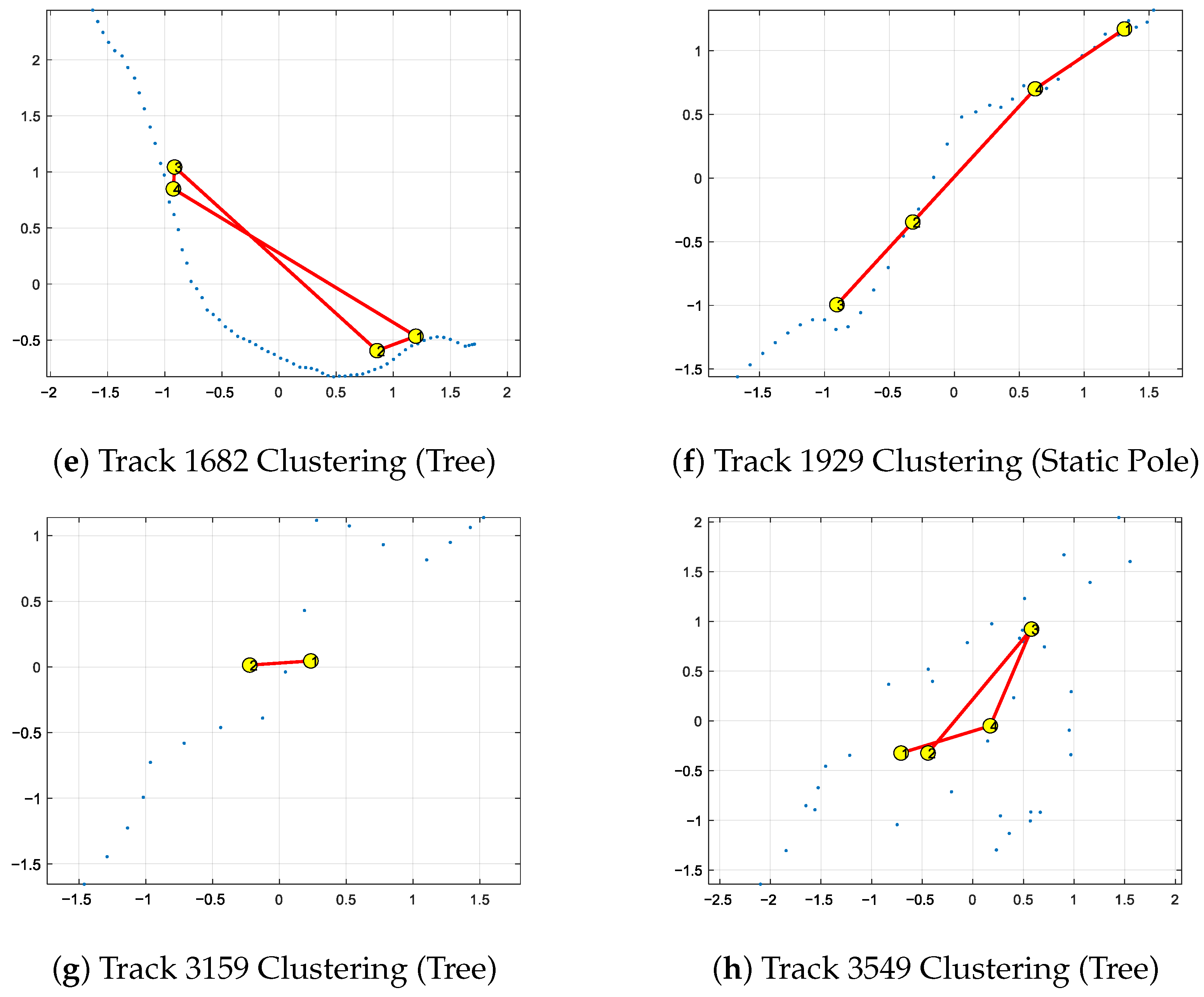
3.2. Implementation Details: Interaction Dictionary and Algorithmic Configurations

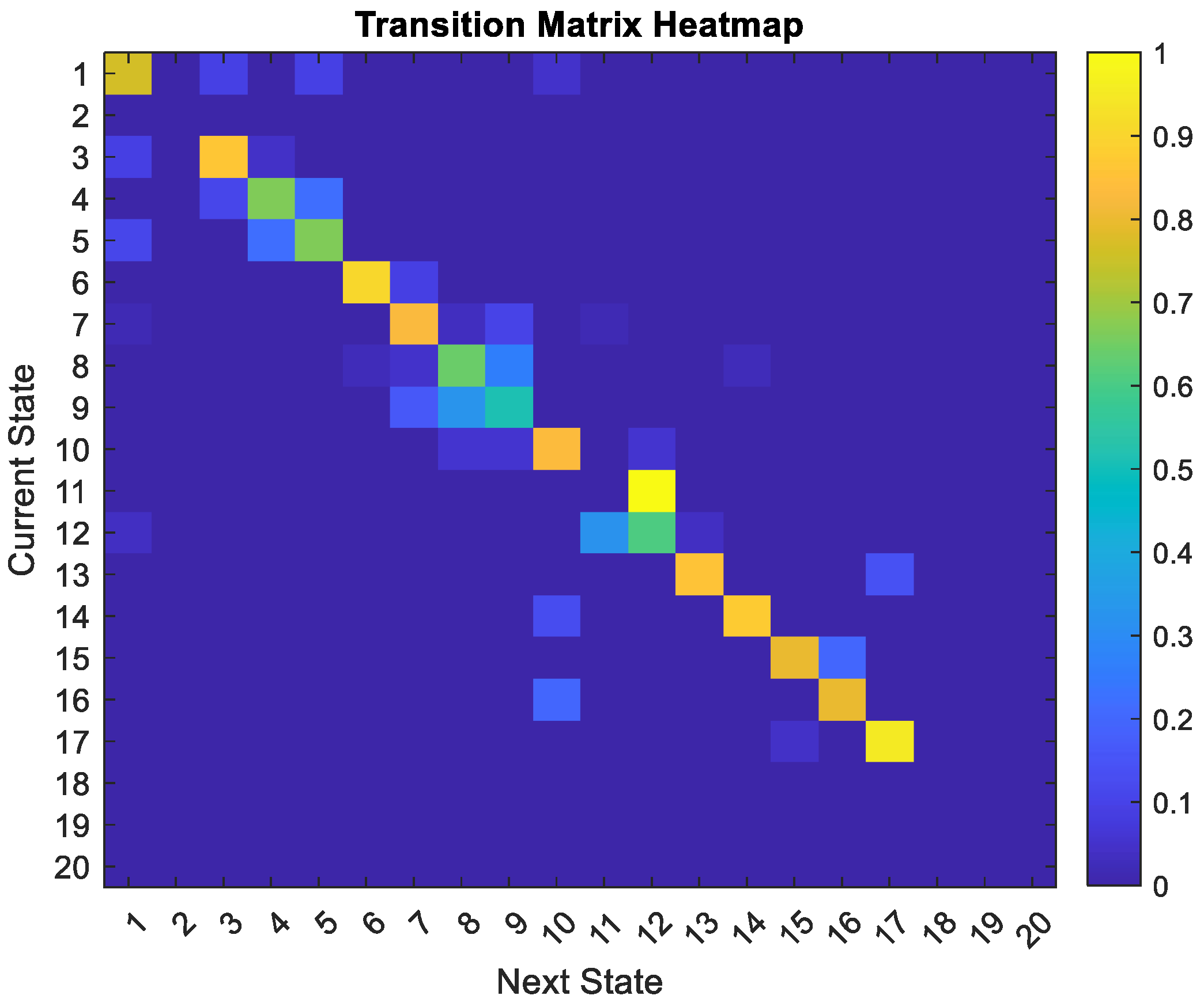
3.2.1. Construction of the Interaction Dictionary

The interaction dictionary encodes the time-dependent relationship between the ego vehicle and each observed track during training. It is constructed using the step-by-step procedure summarized in Table 2.
Each dictionary is constructed for each track during training, and is then combined for simultaneous interactions during testing.

3.2.2. Parameter Configuration for JPDA and GNG

To ensure reproducibility, we detail here the configuration of the JPDA tracker and the GNG algorithm. These components support interaction-based clustering and continuous ego vehicle motion prediction under partial observability.
The GNG network dynamically adjusts its number of nodes based on the complexity of the trajectory during training, with an upper bound of 100 nodes to control overfitting and runtime. The NFF predicts the ego vehicle’s motion by assuming no external forces influence its trajectory resulting in a constant velocity movement. It is a simplified Kalman filter that allows us to estimate future states under a zero acceleration assumption [7]. JPDA parameters were tuned for stability across multi-object scenes. All parameters were empirically selected using the training dataset and are summarized in Table 3.
These values were validated during development and align with established practices in LiDAR-based trajectory modeling.

3.3. Online Testing Phase

In this paper, we extend our previous work by presenting the results of an advanced ego vehicle localization methodology based on combined dictionaries. Our earlier approach [35] used individual interaction dictionaries to localize the ego vehicle through distinct, separate prediction models. In contrast, the methodology described herein integrates multiple track interaction dictionaries into a unified framework, significantly enhancing the robustness of localization.
During the online testing phase, we employ a LiDAR-based dataset consisting of track observations captured in realistic driving scenarios. The localization process leverages vocabulary and interaction dictionaries learned during the offline training phase. The proposed framework comprises distinct steps: track-cluster matching, particle initialization, prediction, and update phases. Importantly, the integration of combined interaction dictionaries allows for the simultaneous handling of multiple static tracks, periods without observations, and isolated track interactions. The DBN model during testing for seperate tracks predictions is shown in Figure 6.
The use of an MJPF in the online phase is motivated by the hybrid nature of the localization task, which involves both discrete transitions across interaction clusters and continuous ego motion estimation. Traditional Kalman filters, while efficient, rely on linear motion assumptions and cannot adapt to abrupt mode transitions or temporary observation loss. On the other hand, standard particle filters, although capable of handling nonlinearity, do not explicitly model structured mode switching [51]. MJPF addresses these limitations by combining discrete state inference with continuous filtering. It uses a particle filtering mechanism to sample over a joint continuous-discrete state space and applies Kalman updates within each cluster mode. This hybrid strategy allows the model to dynamically switch between clusters based on transition probabilities learned from the interaction dictionaries, to maintain robust trajectory estimation during occlusion or missing data, and to utilize statistical priors for cluster-specific correction. As a result, MJPF significantly improves robustness and accuracy compared to conventional filtering methods, especially in scenarios involving overlapping tracks, intermittent visibility, or multi-tracks interaction.

3.4. Localization with Combined Dictionary

In our earlier work, we introduced an MJPF approach for localizing an AV using static LiDAR-based landmarks. Specifically, the results presented an in-depth analysis where individual track dictionaries (e.g., buildings, poles, trees) were used to estimate ego-vehicle trajectories. It was demonstrated that each track, treated separately, could yield highly accurate localization results if treated as a stable landmark.
However, real-world driving scenarios are far more complex. Multiple static tracks can appear simultaneously, and certain time intervals might exist with no observations. This motivates the need to combine the information contained in the different dictionaries (one dictionary per track) into a unified framework. By doing so, we can better handle the following situations:
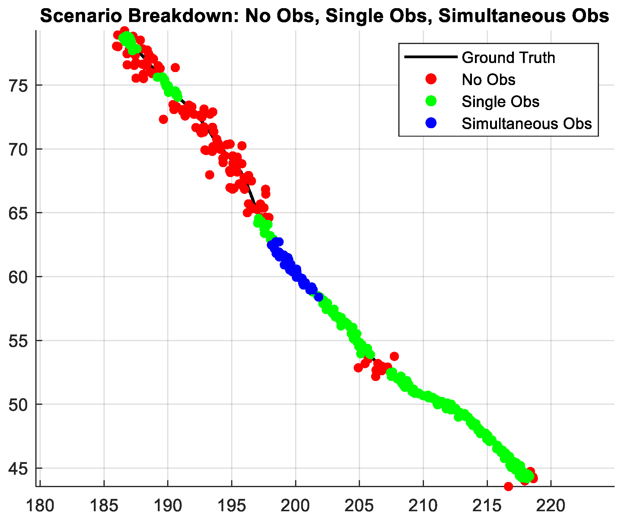
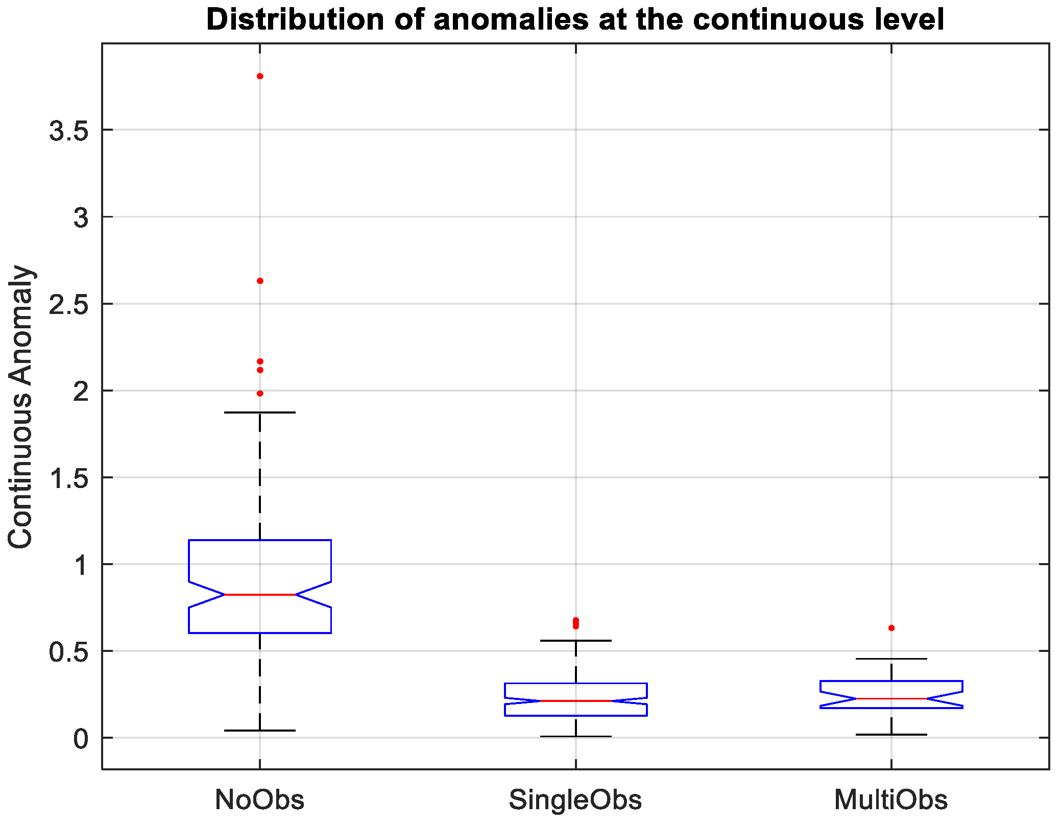
  • Simultaneous Track Interactions: When multiple static tracks are observed at the same instant, combining dictionaries can refine ego-vehicle position estimates by leveraging cross-track constraints.
  • Extended No Observation Periods: In some time intervals, no new LiDAR observations of static tracks may be available (e.g., occlusion or sensor dropout). Incorporating combined dictionaries can help maintain stable localization by relying on prior learned interactions across multiple tracks.
  • Isolated Track Interactions: Even when only one track is observed, the combined dictionary framework can cross-validate with other track dictionaries (now unused) to check for consistency, thereby reducing ambiguity.

3.4.1. Steps to Create a Combined Dictionary

Step 1: Concatenate All Track Dictionaries. We initialize I combined as the union of all I k :
I combined = k = 1 K I k
where K represents the six static tracks considered.
Step 2: Remove Duplicate or Overlapping Entries. At certain time instants t, interactions may occur with multiple tracks. These are simultaneous interactions. If the same ego-vehicle cluster C ego is repeated with minor variations, we merge or remove duplicates to ensure the dictionary remains concise.
Step 3: Store Track-Specific Indices. To preserve which track each interaction came from, we store an additional track ID label in each dictionary entry:
t , C ego , C track , L , x , y , track _ ID .
This helps in quickly referencing the relevant transition matrices or covariance structures for that track.
Step 4: Recompute Interaction Statistics. For each unique pair ( C ego , C track ) , we can compute:
( μ x , μ y , Σ x , Σ y )
to represent the mean and covariance of the ego positions ( x , y ) encountered in those interactions. These statistics become vital when updating or predicting the ego state from the combined dictionary.

3.4.2. Bhattacharyya Distance to Match Observed Tracks

Whenever a new observed track z t obs appears in the LiDAR data, we must determine which track cluster it corresponds to in the combined dictionary I combined . We use the Bhattacharyya distance d B :
d B z t obs , z t cluster = 1 8 z t obs z t cluster Σ 1 z t obs z t cluster + 1 2 ln det ( Σ ) det ( Σ obs ) det ( Σ cluster ) ,
where
Σ = 1 2 Σ obs + Σ cluster .
Here, z t obs denotes the observed track position vector at time t, while z t cluster represents the mean position of a cluster in the combined dictionary. Similarly, Σ obs and Σ cluster are the covariance matrices corresponding to the observed track and the cluster, respectively. The matrix Σ is the average covariance, balancing the uncertainty between the two.
We assign the observed track to the cluster S v t that yields the minimum Bhattacharyya distance:
S v t = arg min S I combined d B z t obs , z t cluster .
Thus, the combined dictionary still uses the same track-cluster matching but across all possible track entries from 1 to K.

3.4.3. Particle Initialization for Multiple Tracks

At t = 1 , if the AV observes M different static tracks from LiDAR, we sample N particles for each track m = 1 , , M , following:
z 1 , n track , m N M S v 1 ( m ) , Q S v 1 ( m ) ,
where S v 1 ( m ) is the matched dictionary entry for track m. Here, M S v 1 ( m ) and Q S v 1 ( m ) denote the mean and covariance of the matched cluster, respectively.
For the ego vehicle, we combine all relevant dictionary means:
z 1 , n ego N M ¯ ego , Q ¯ ego ,
where
M ¯ ego = 1 M m = 1 M M S v 1 ( m ) ego , Q ¯ ego = diag σ x 2 , σ y 2 ,
is an averaged or fused initial guess for the ego vehicle. Here, σ x 2 and σ y 2 represent predefined variances for the initial ego position uncertainty along the x and y axes.

3.4.4. Prediction Phase (Per Track and Ego Vehicle)

Each track m evolves via:
z t + 1 | t , n track , m = A track S t , n ( m ) z t | t , n track , m + w t track , m ,
where A track S t , n ( m ) represents the learned dynamic model matrix for track m at time t, and w t track , m is the process noise accounting for motion uncertainty.
Meanwhile, the ego vehicle evolves as:
z t + 1 | t , n ego = A ego S t , n ( 1 ) , , S t , n ( M ) z t | t , n ego + B ego S t , n ( 1 ) , , S t , n ( M ) + w t ego ,
where A ego and B ego depend on all matched track indices ( 1 , , M ) to incorporate multiple dictionary entries. Here, w t ego denotes the process noise affecting the ego vehicle prediction.

3.4.5. Update Phase (Measurements + Combined Interaction)

Upon receiving LiDAR measurements a t track , m for each observed track m, we update track m via a Kalman Filter correction:
z t | t , n track , m = z t | t 1 , n track , m + K t track , m a t track , m C track S t , n ( m ) z t | t 1 , n track , m ,
where K t track , m denotes the Kalman gain for track m, and C track S t , n ( m ) represents the observation model matrix associated with the matched cluster.
For the ego vehicle, we combine the influence of all observed tracks using the interaction dictionaries:
z t | t , n ego = z t | t 1 , n ego + m = 1 M D ( m ) S t , n ( m ) z t | t , n track , m + E ( m ) S t , n ( m ) ,
where D ( m ) S t , n ( m ) and E ( m ) S t , n ( m ) are the track-specific adjustment matrices and biases obtained from the combined dictionary for track m.

3.4.6. DBN Structure During Training

The training phase of DBN as shown in Figure 7 incorporates data from both the odometry sensor and the LiDAR training dataset to build a robust model of the environment. The odometry sensor provides precise ego vehicle positions, forming a reliable foundation for motion estimation, while the LiDAR dataset captures interactions with surrounding objects. From this data, six static tracks (corresponding to stationary objects such as buildings, poles, and trees) were classified and stored for future reference.
The DBN in the training phase operates as follows:
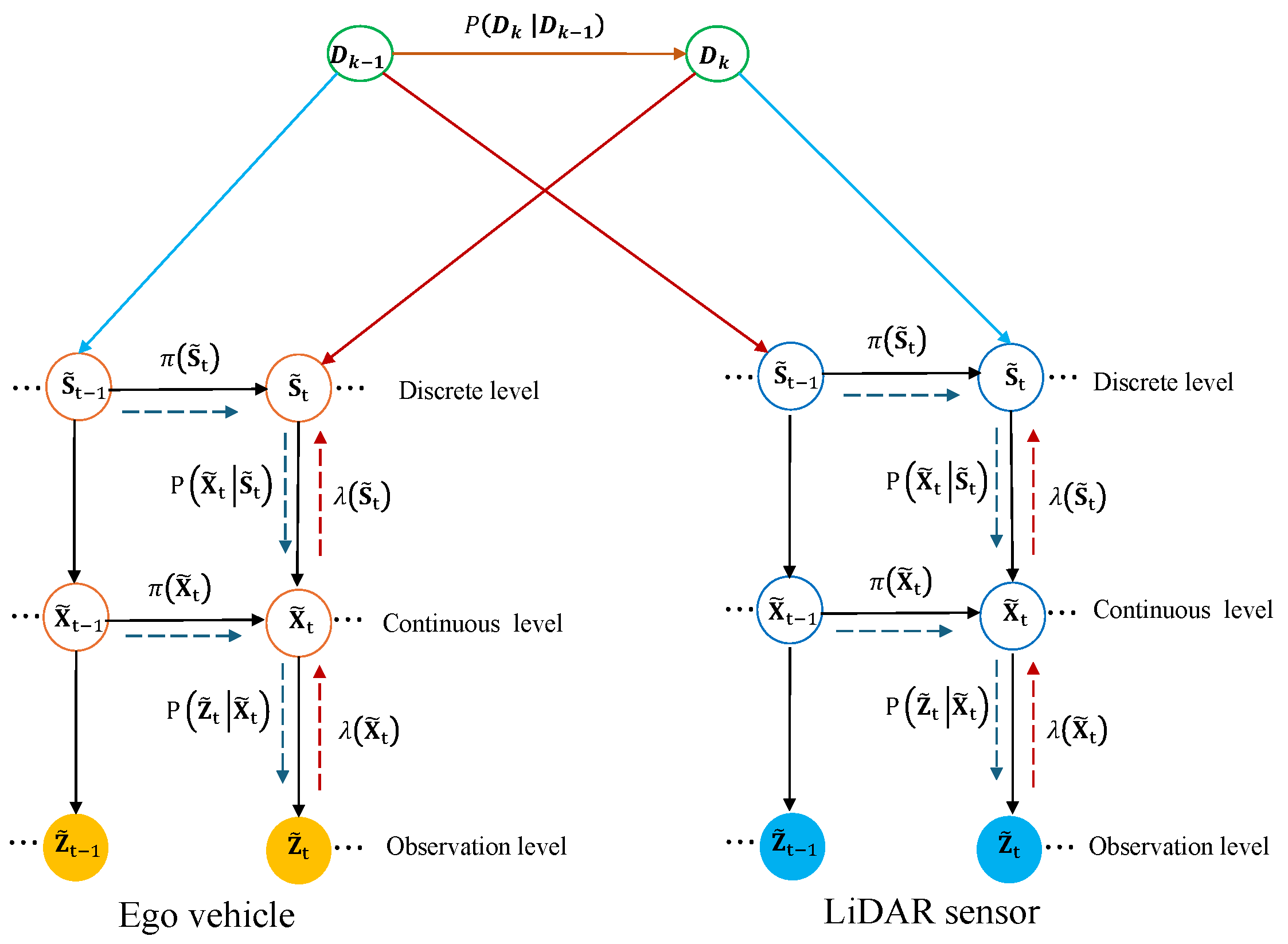
  • Sensor Integration: The lower-level nodes in the DBN represent the ego vehicle’s state, including its hidden state S ˜ 0 , predicted position X ˜ 0 , and observed position Z ˜ 0 . These nodes are connected via transition probabilities P ( X ˜ 0 | S ˜ 0 ) , modeling the odometry-based motion dynamics.
  • LiDAR-Based Track Classification: At the track level, the DBN models individual static tracks, such as S L T ˜ 1 , where S L T ˜ 1 represents the hidden state of the track and X L T ˜ 1 represents its observed position. Transition probabilities P ( X L T ˜ 1 | S L T ˜ 1 ) capture the temporal evolution of these static objects in the LiDAR dataset.
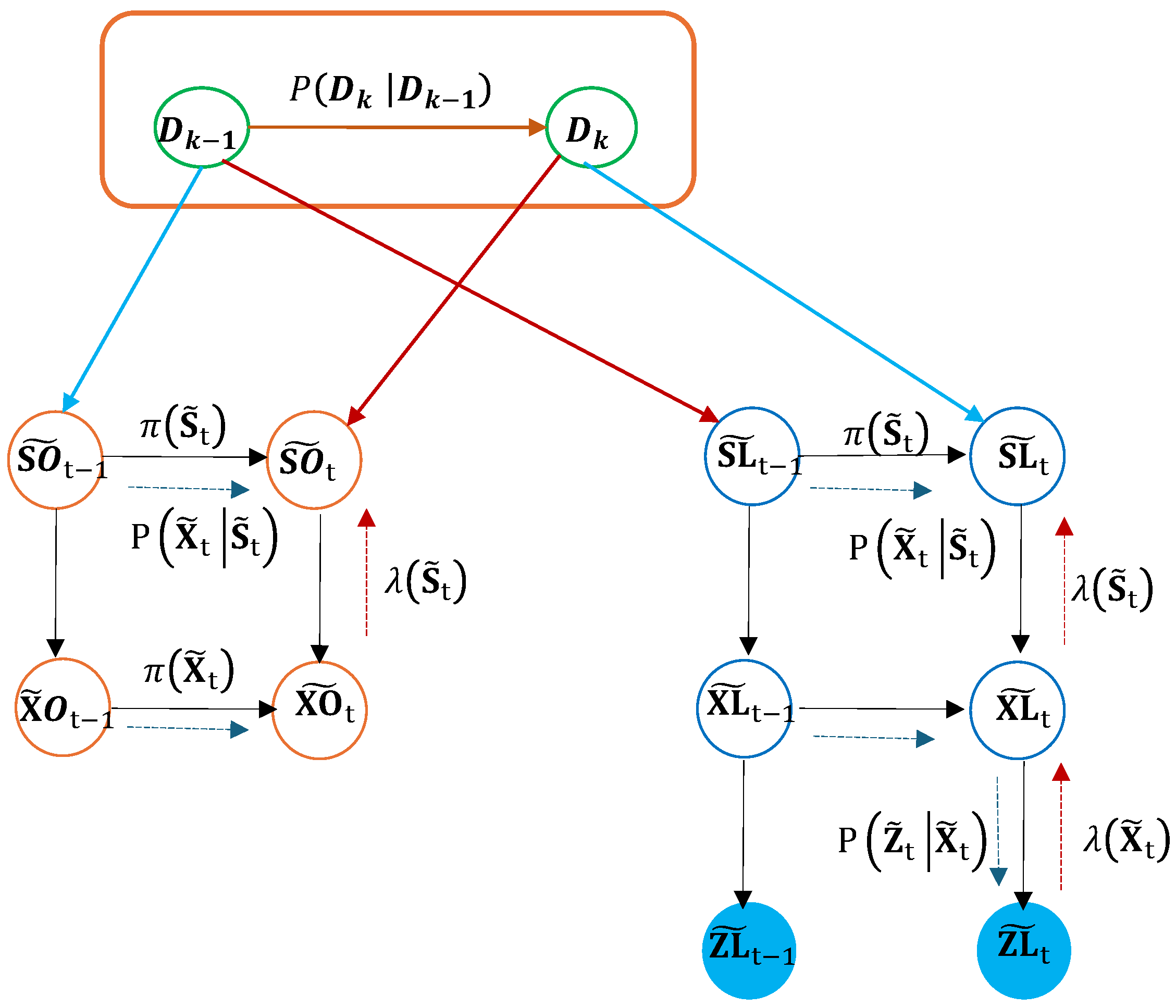
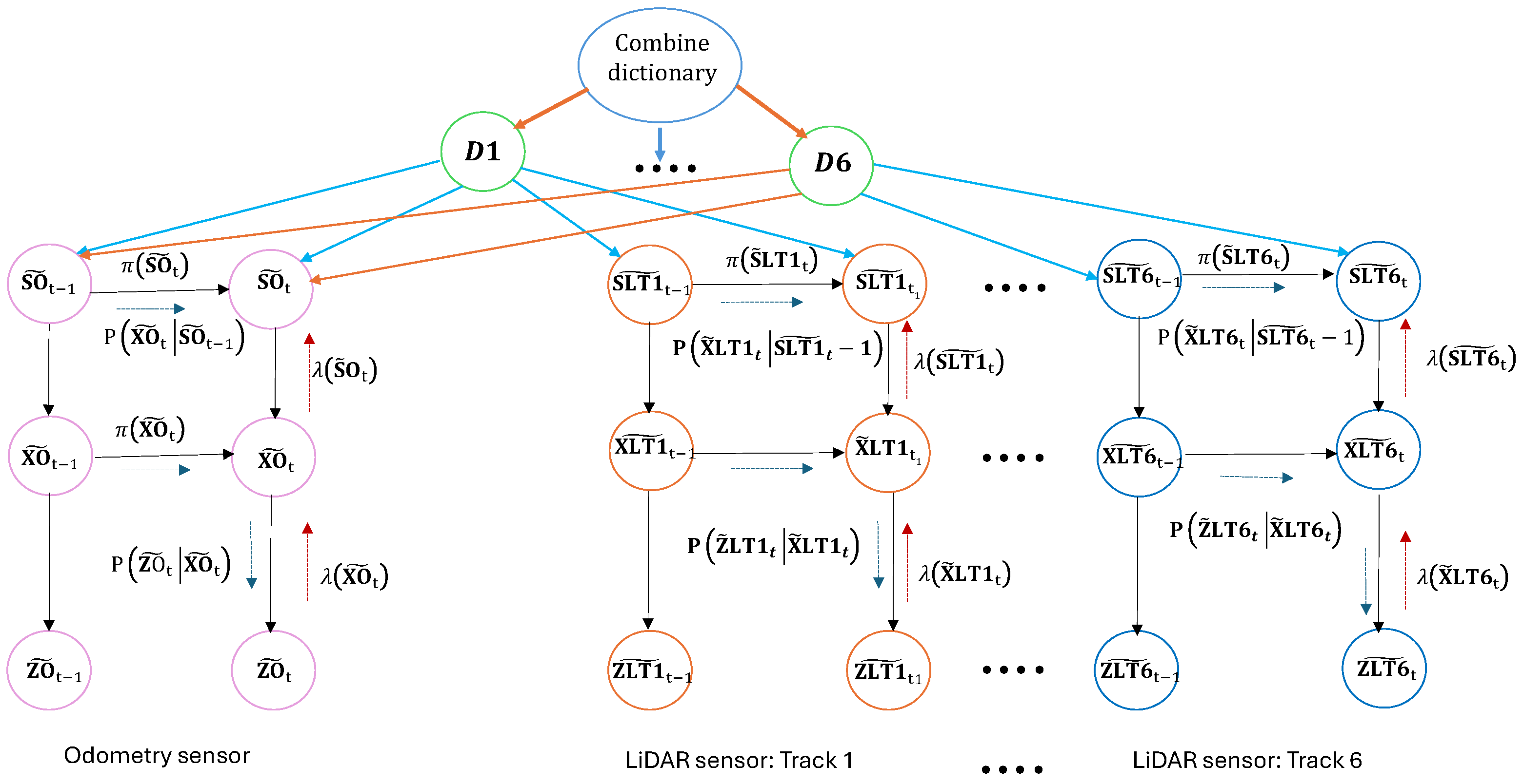
  • Dictionary Fusion: A higher-level node integrates the outputs of all track-level nodes into a unified combined dictionary. This dictionary serves as a probabilistic repository of interactions between the ego vehicle and the classified tracks. It encodes cross-track consistency and enables robust ego position estimations across different scenarios.
This approach ensures that the training phase produces a comprehensive model of the environment, capturing both the static structure and the temporal dynamics of track interactions. The combined dictionary becomes a central component for downstream testing.

3.4.7. DBN Structure During Testing

The testing phase of DBN as shown in Figure 8 is designed to operate without the odometry sensor, relying solely on the LiDAR testing dataset for ego vehicle localization. The testing DBN builds on the insights learned during training, focusing on matching observed tracks to the pre-classified tracks and using this information to estimate the ego vehicle’s position.
The DBN for testing operates as follows:
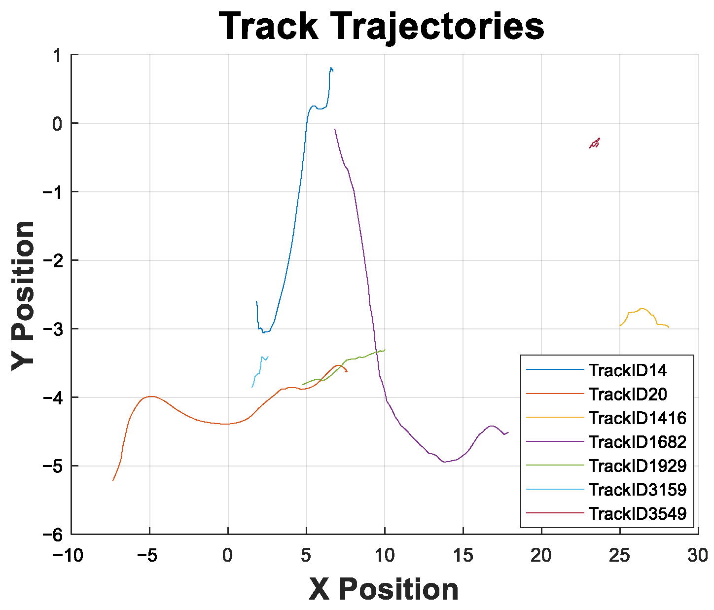
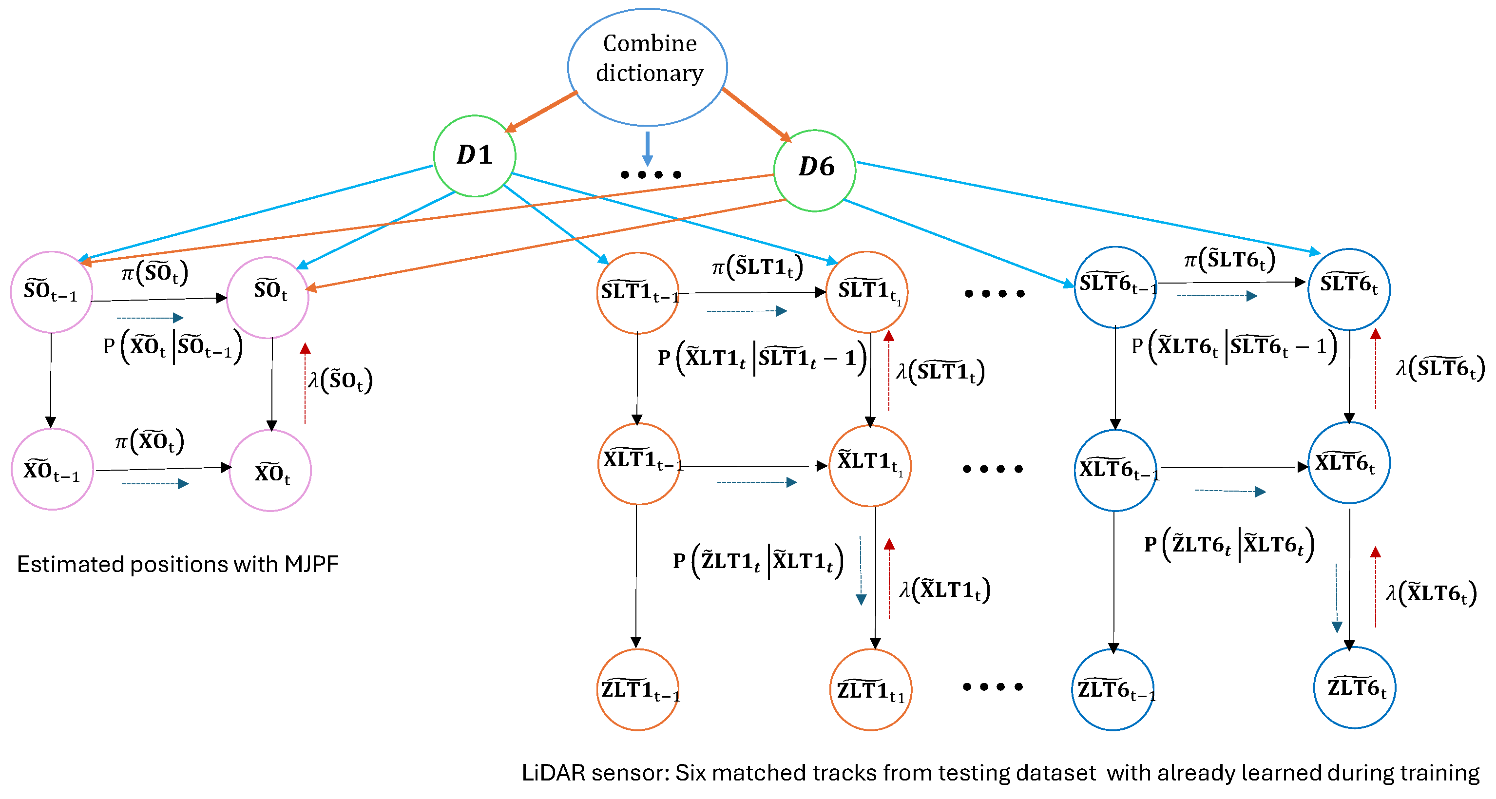
  • Track Matching: Observed tracks in the LiDAR testing dataset are matched with the learned static tracks using the Bhattacharyya distance. This step ensures that the six static tracks identified during training are accurately re-associated with their counterparts in the testing environment, which shares a similar structure.
  • Prediction with MJPF: Once the tracks are matched, the MJPF predicts the ego vehicle’s positions. The MJPF leverages the matched tracks as static references, using the learned motion dynamics and interaction models to estimate the ego state.
  • Dictionary Fusion for Robust Estimation: The matched track dictionaries are combined into a unified dictionary, as in the training phase. This fused dictionary incorporates all static tracks and provides probabilistic corrections to the MJPF predictions, ensuring that the ego vehicle’s trajectory remains consistent with the observed environment.
  • Final Ego Position Estimation: The leftmost nodes of the DBN represent the final estimated positions of the ego vehicle. These nodes aggregate probabilistic influences from all matched tracks and the fused dictionary, enabling accurate localization even in the absence of direct odometry input.

4. Results and Discussion

In this section, we present and analyze the results obtained from our proposed methodology, structured into two distinct subsections. First, we evaluate the classification performance, demonstrating the effectiveness of our approach in distinguishing between static and dynamic tracks based on LiDAR data. This classification is fundamental for accurate localization, as static tracks serve as reliable landmarks while dynamic tracks provide crucial contextual information about the surrounding environment. In the second part we present the results of a more generalized approach by incorporating a combined dictionary that integrates multiple static track interactions. This approach enables a more robust localization framework by leveraging multiple reference tracks simultaneously, addressing challenges such as no observation gaps and multi-track interaction scenarios. Through this structured evaluation, we aim to demonstrate the advantages and limitations of each approach while providing insights into how track classification and probabilistic modeling contribute to improving ego vehicle localization in LiDAR-based environments.

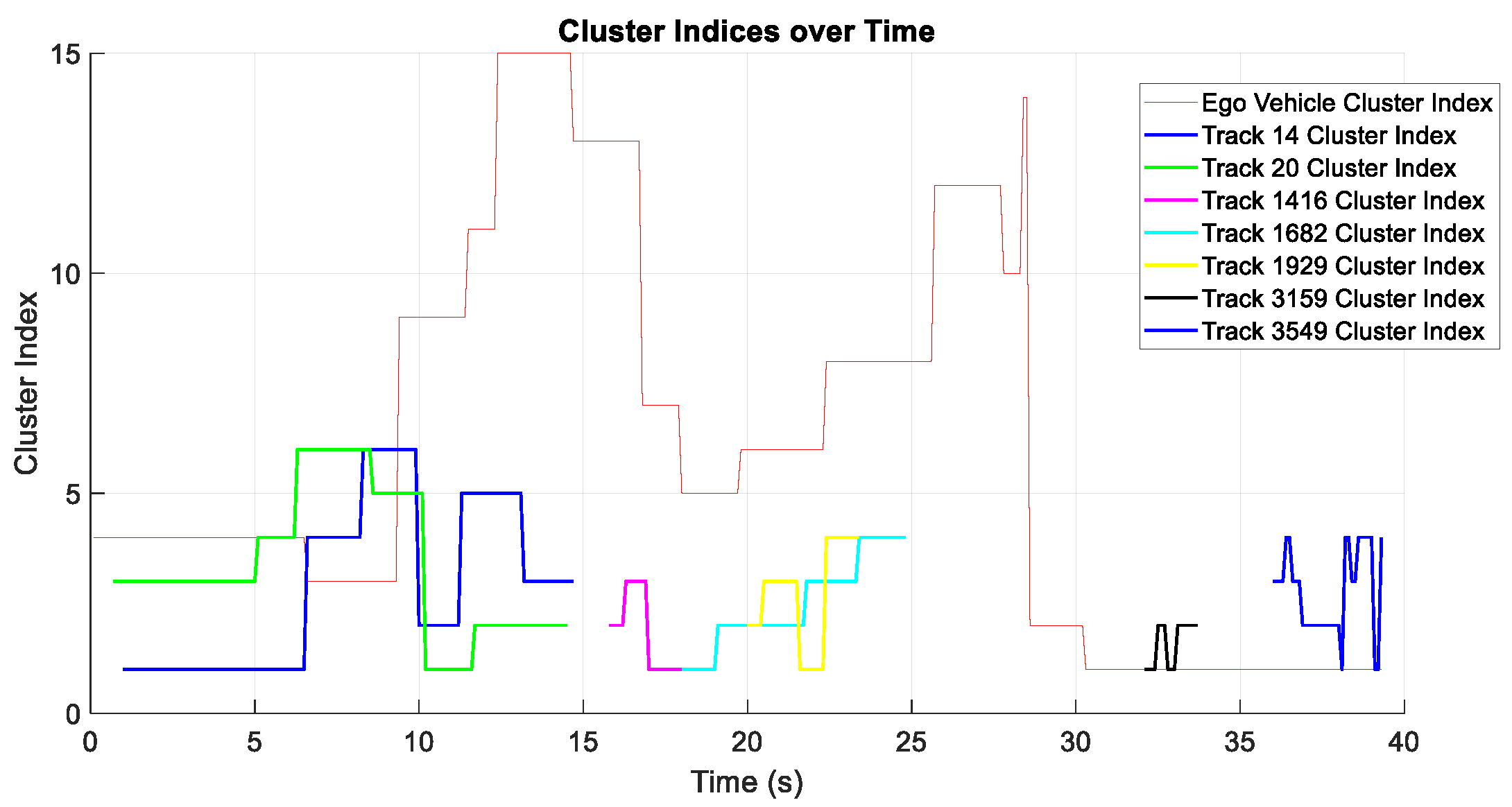
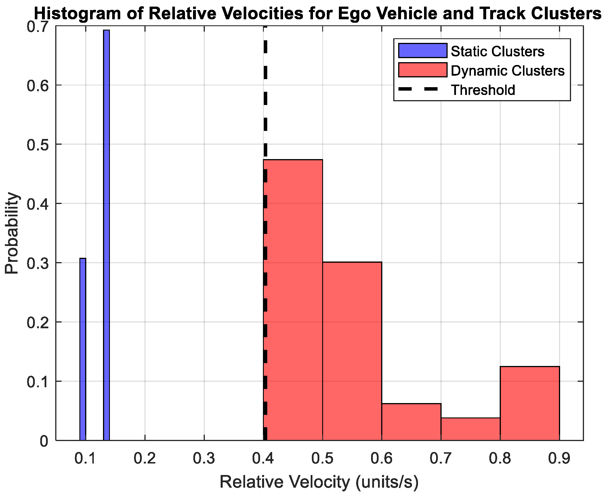
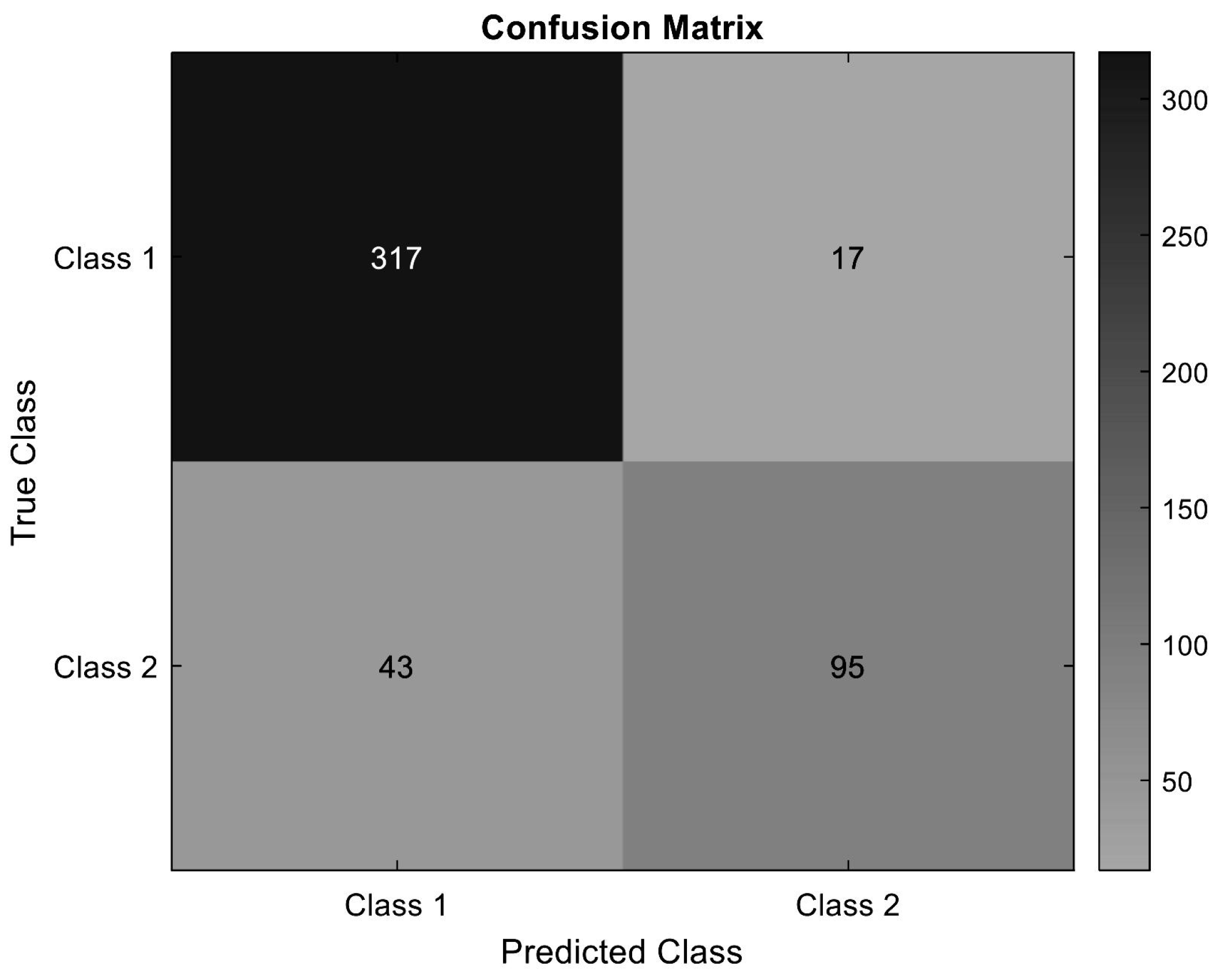
4.1. Classification Results

Using the minimum distance between the current positions of the ego vehicle and predefined cluster centroids of track positions, the nearest cluster indices were determined for both the ego vehicle and the tracks at each timestamp. A comprehensive overview of the dynamics of the interaction between the ego vehicle and the surrounding tracks is shown in Figure 9. At various time instants, it details when each track interacts with the ego vehicle. This figure depicts both scenarios in which multiple tracks interact with the ego vehicle simultaneously, as well as scenarios in which separate tracks engage at different intervals.
For the purpose of distinguishing static clusters from dynamic clusters, the threshold is calculated by accumulating all relative velocities of interactions in a histogram, and calculating the mean plus standard deviation. An adaptive threshold method for detecting human motion is based on the method proposed in [52]. A histogram is shown in Figure 10: dynamic velocities appear to the right of the threshold, and static velocities appear to the left. Some dynamic points are misclassified as static points and vice versa, but our model correctly classifies most of the points.
Our proposed method has been validated over time as shown in Figure 11, demonstrating both static and dynamic classification accuracy. We are able to distinguish between static clusters (blue points below the threshold line) and dynamic clusters (red points above the threshold line). Using this validation, we are able to confirm that the threshold we chose reliably classifies interactions, as we are already familiar with the expected behavior of track clusters over time. As a result, the majority of points are correctly classified, demonstrating the effectiveness of our model.
Our classification model is further validated by computing the confusion matrix [53] shown in Figure 12. We compare the true labels (dynamic or static) with the predicted labels. A true class is defined based on known interactions, such as Track 14 is being dynamic, while the other tracks remain static. The predicted classes are determined using our classification algorithm, which utilizes threshold values derived from the mean and standard deviations of the relative velocities.
The confusion matrix shows the following metrics.
  • True positive (TP): The 317 dynamic interactions are correctly classified.
  • True negative (TN): The 95 static interactions are correctly classified.
  • False positive (FP): 43 static interactions are misclassified as dynamic.
  • False negative (FN): 17 dynamic interactions are misclassified as static.
The results of the performance metrics are shown in Table 4. The classification model we developed achieved an accuracy of 87% in classifying static and dynamic tracks, demonstrating its effectiveness. Based on the high recall of 94%, most dynamic interactions are correctly identified. A precision of 88% indicates a good balance between true positives and false positives. The F1 score of 91% indicates that our model exhibits a strong balance between precision and recall, which confirms the robustness of the model. Following the same methodological approach, we extended our classification algorithm to the KITTI dataset [54], which comprises 1101 LiDAR frames. The evaluation metrics derived from this dataset are summarized in Table 4. The results confirm the reliability of our approach, as it maintains consistent performance across both the iCAB and KITTI datasets.

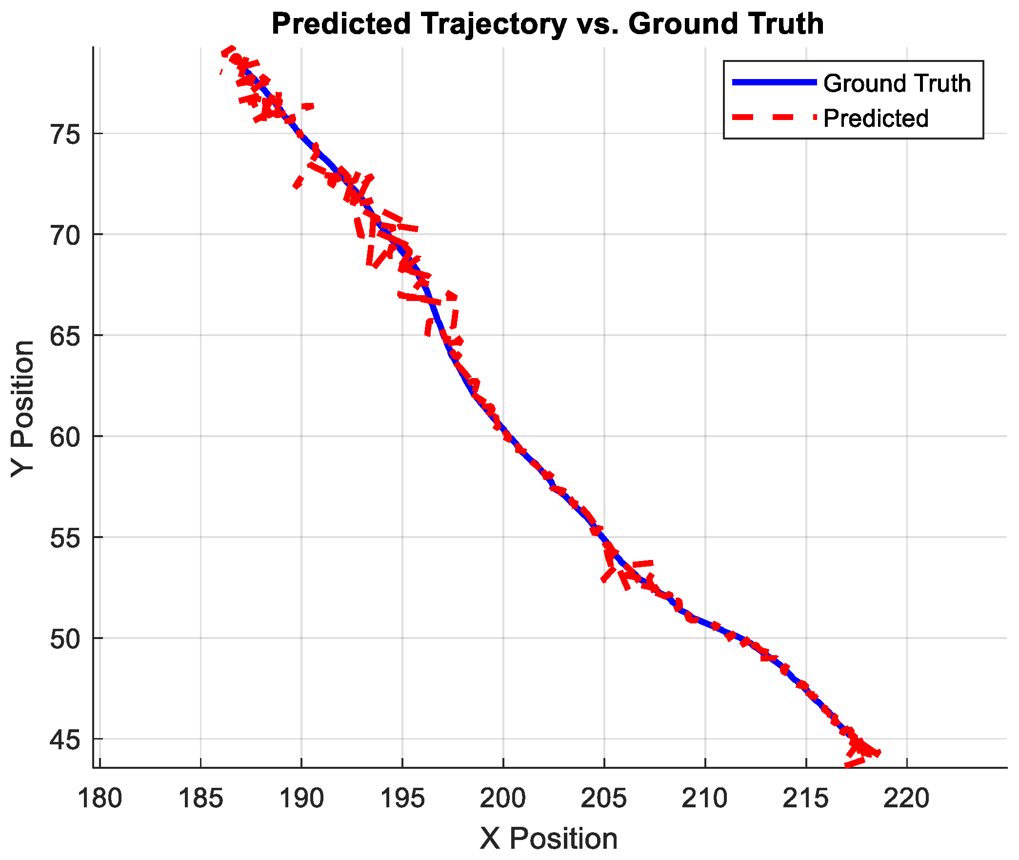
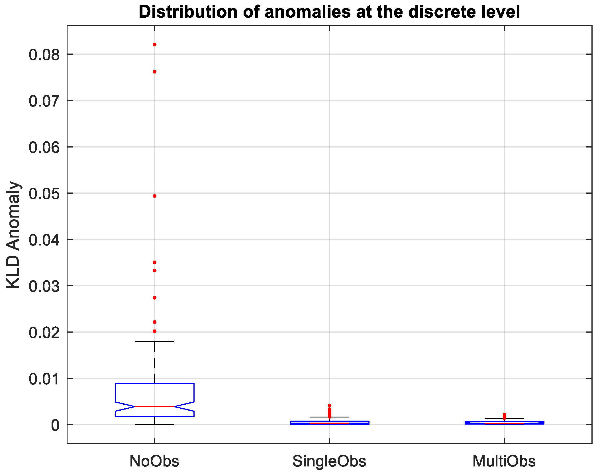
4.2. Localization Results Using a Combined Dictionary

This subsection presents the localization results of our proposed methodology using a combined dictionary approach, effectively leveraging multiple static landmarks for robust AV localization. The combined dictionary enhances the filter’s predictive capability under varying environmental scenarios such as simultaneous multi-track observations, periods without sensor inputs (no-observation intervals), and isolated single-track updates.
Figure 13 presents a direct comparison between the predicted ego vehicle trajectory (red dashed line) and the ground truth (solid blue line). It demonstrates that the combined dictionary approach significantly reduces localization drift, particularly in comparison to periods without observations. Furthermore, Figure 14 illustrates the predicted ego states under multiple interaction scenarios, depicted in different colors to clearly differentiate state transitions. The consistency between predicted and actual trajectories validates the robustness of using a combined dictionary in complex scenarios.
The corresponding transition matrix in Figure 15 highlights minimal off-diagonal components, signifying accurate and stable state transitions. This observation suggests that the combined dictionary is accurately capturing the relationships and maintaining consistency across multiple landmark interactions, thereby ensuring stable localization results.
To provide deeper insights into localization performance, we analyzed two types of anomalies: continuous-level anomalies (CLA) and discrete-level anomalies (KLDA).
In our context, continuous-level anomalies (CLA) measure the difference between the MJPF’s predicted continuous states (e.g., positions of the ego vehicle derived from the combined dictionary) and the actual LiDAR measurements. Figure 16 displays the continuous-level anomalies across the test duration (41.5 s). Initially (0–2 s), a high anomaly peak exceeding 2.0 is observed due to insufficient initialization data, causing early filter misalignment. However, the anomaly reduces significantly as more measurements are integrated, indicating effective state correction by the MJPF. Notably, at approximately 15 s (frame 150), a significant spike occurs due to the ego vehicle initiating a complex overtaking maneuver, causing a large deviation between predicted and observed states. Subsequent spikes around 28 s and 33 s similarly indicate transitions from periods without observations to sudden reintroduction of sensor data, resulting in abrupt corrections of the filter’s predictions.
Discrete-level anomalies (KLDA) represent discrepancies at a higher level, specifically in the discrete state assignments or “cluster labels”. As the MJPF uses predefined cluster assignments from the combined dictionary, KLDA measures the divergence between predicted discrete states (clusters) and observed track distributions. Figure 17 illustrates these discrete anomalies. Initially, discrete anomalies remain low (0–14 s), indicating consistent alignment between predicted and observed clusters. However, during dynamic interactions (especially the critical overtaking maneuver at 15 s), significant discrete anomalies emerge due to abrupt mismatches in cluster assignments. Subsequent spikes at 28 s and 33 s coincide again with intervals of no observations, reinforcing how intermittent sensor data availability significantly impacts discrete-state estimation consistency.
Figure 18 and Figure 19 provide boxplots summarizing the distributions of continuous and discrete anomalies across three distinct scenarios: No Observation (NoObs), Single Track Observation (SingleObs), and Multiple Track Observations (MultiObs). In Figure 18, the NoObs scenario shows a higher median and a larger spread in continuous anomaly values, indicative of increased uncertainty and drift when relying solely on predictive models without sensor updates. Conversely, scenarios involving SingleObs and MultiObs demonstrate tighter distributions around lower anomaly values, clearly illustrating the stabilizing effect of receiving even sparse landmark observations.
Similarly, the discrete-level anomalies depicted in Figure 19 present a parallel trend: periods without observations (NoObs) have greater variance and multiple outliers due to the inability to accurately assign discrete states without regular sensor feedback. Conversely, the SingleObs and MultiObs scenarios show reduced dispersion and lower median anomaly values, emphasizing the effectiveness of consistent or even intermittent landmark observations in maintaining accurate discrete state estimations.
Overall, these findings underscore the value of our combined dictionary-based MJPF, which ensures robust localization even under challenging conditions by effectively integrating continuous and discrete state predictions. The anomaly analyses clearly demonstrate the MJPF’s adaptability in dynamic environments, significantly contributing to reliable ego-vehicle navigation and localization performance.

4.3. Computational Efficiency Analysis

To assess the practical feasibility of the proposed localization framework, we conducted a detailed evaluation of its runtime performance on a standard non-GPU-enabled system. The implementation was executed on a laptop equipped with an Intel Core i7-7500U CPU @ 1.80 GHz, 16 GB RAM, and running Windows 11 Home (64-bit).
Unlike image-based localization approaches, our system operates on LiDAR point cloud frames, where each frame corresponds to a 3D scan obtained from a Velodyne VLP-16 sensor. The average computation time for processing a single point cloud frame during the online testing phase was measured to be approximately 41 milliseconds, enabling a processing rate of around 24 frames per second (FPS). This confirms the potential of our framework for near real-time autonomous vehicle localization tasks.
To ensure computational efficiency, the following optimizations were applied:
  • Cluster Matching Optimization: Only the most relevant clusters are matched using Bhattacharyya distance, significantly reducing the number of comparisons during track association.
  • Selective Kalman Updates: Kalman filter prediction and update steps are performed exclusively for those clusters actively involved in interactions, avoiding unnecessary computations.
  • Efficient MJPF Design: The Markov Jump Particle Filter marginalizes linear components within the state space, which reduces the number of particles and accelerates inference.
In terms of memory scalability, the interaction dictionaries grow linearly with the number of observed tracks and frames in a given environment. Each dictionary entry encodes one frame-level interaction, making the size of the dictionary proportional to the temporal span and the number of interacting static objects. For example, in our current setup, combining six track dictionaries results in a total memory footprint of less than 15 MB. During testing, only the relevant time slices are queried from these pre-indexed dictionaries, ensuring low-latency access. Thus, even when scaled to more complex scenes with dozens of static landmarks, the structure remains computationally efficient. This is due to the selective querying and use of spatial hashing for dictionary access, supporting real-time performance in extended urban driving scenarios.
These design strategies ensure that the proposed approach remains computationally feasible even on resource-constrained hardware, and can be potentially extended to embedded systems with comparable performance capabilities.

4.4. Ablation Study of Core Components

To evaluate the importance of individual components within the proposed localization framework, we conducted an ablation study by progressively removing or altering key modules. Each ablation scenario was tested under identical conditions using the LiDAR-based point cloud testing dataset described earlier (415 frames). The average localization error was recorded for each setting and compared to the full system.
The results in Table 5 show that both the MJPF and the combined dictionary substantially enhance localization accuracy (the best result is highlighted in bold). Removing the MJPF leads to increased error due to the lack of stochastic reasoning across cluster transitions, while omitting the combined dictionary weakens the system’s ability to handle simultaneous track observations and sensor dropout scenarios. The highest error occurs when both components are disabled, confirming their combined necessity.
These findings reinforce the robustness and necessity of our proposed system architecture in ensuring reliable localization across diverse real-world scenarios.

5. Conclusions

This paper introduced a robust LiDAR-based methodology for object classification and ego vehicle localization, employing a generative model framework that includes DBNs and interaction dictionaries. The proposed method achieved a high classification accuracy, validating the efficacy of our threshold-based classification technique in distinguishing static and dynamic interactions. Furthermore, our localization approach, which integrates a combined dictionary and utilizes the MJPF, demonstrated significant improvements in reducing positional drift and maintaining accurate localization, even under challenging scenarios such as simultaneous multi-track interactions and periods without observations. The overall results confirm the robustness and effectiveness of the proposed methodology for AV navigation, providing a solid foundation for enhanced real-world application scenarios. In future work, we aim to apply our full localization framework, beyond classification, on large-scale public datasets such as KITTI. This includes building track-based dictionaries using LiDAR-only data from KITTI sequences and adapting the MJPF framework to test real-world scalability in unstructured and urban driving environments.

Author Contributions

Investigation, M.A., P.Z., D.M.G., L.M. and C.R.; Validation, M.A., P.Z., D.M.G., L.M. and C.R.; Writing—original draft, M.A., P.Z., D.M.G., L.M. and C.R. All authors have read and agreed to the published version of the manuscript.

Funding

This research was partially funded by the European Union’s Horizon Europe research and innovation programme under the Grant Agreement No. 101121134 (B-prepared), and by the European Union—NextGenerationEU and by the Ministry of University and Research (MUR), National Recovery and Resilience Plan (NRRP), Mission 4, Component 2, Investment 1.5, project “RAISE—Robotics and Al for Socio-economic Empowerment” (ECS00000035). This research was also funded by the Spanish Government under Grants: PID2021-124335OB-C21, PID2022-140554OB-C32, TED2021-129485B-C44 and PDC2022-133684-C31.

Institutional Review Board Statement

Not applicable.

Informed Consent Statement

Not applicable.

Data Availability Statement

The data included in this study are available on request from the corresponding author.

Conflicts of Interest

The authors declare no conflict of interest.

List of Abbreviations

AVAutonomous Vehicle
LiDARLight Detection and Ranging
MJPFMarkov Jump Particle Filter
DBNDynamic Bayesian Network
GNGGrowing Neural Gas
JPDAJoint Probabilistic Data Association
NFFNull Force Filter
KFKalman Filter
PFParticle Filter
CLAContinuous-Level Anomaly
KLDAKullback–Leibler Divergence Anomaly
KITTIKarlsruhe Institute of Technology and Toyota Technological Institute dataset
MSEMean Squared Error
RMSERoot Mean Squared Error
DBSCANDensity-Based Spatial Clustering of Applications with Noise
CIFsCovariance Intersection Filters
VAEVariational Autoencoder
CMJPFCoupled Markov Jump Particle Filter

References

  1. Yurtsever, E.; Lambert, J.; Carballo, A.; Takeda, K. A survey of autonomous driving: Common practices and emerging technologies. IEEE Access 2020, 8, 58443–58469. [Google Scholar] [CrossRef]
  2. Chong, Y.S.; Tay, Y.H. Abnormal event detection in videos using spatiotemporal autoencoder. In Proceedings of the Advances in Neural Networks-ISNN 2017: 14th International Symposium, ISNN 2017, Sapporo, Hakodate, and Muroran, Hokkaido, Japan, 21–26 June 2017; Proceedings, Part II 14. Springer: Berlin/Heidelberg, Germany, 2017; pp. 189–196. [Google Scholar]
  3. Nozari, S.; Krayani, A.; Marin, P.; Marcenaro, L.; Gomez, D.M.; Regazzoni, C. Modeling autonomous vehicle responses to novel observations using hierarchical cognitive representations inspired active inference. Computers 2024, 13, 161. [Google Scholar] [CrossRef]
  4. Kotseruba, I.; Tsotsos, J.K. 40 years of cognitive architectures: Core cognitive abilities and practical applications. Artif. Intell. Rev. 2020, 53, 17–94. [Google Scholar] [CrossRef]
  5. Morin, A. Levels of consciousness and self-awareness: A comparison and integration of various neurocognitive views. Conscious. Cogn. 2006, 15, 358–371. [Google Scholar] [CrossRef] [PubMed]
  6. Alemaw, A.S.; Slavic, G.; Zontone, P.; Marcenaro, L.; Gomez, D.M.; Regazzoni, C. Modeling Interactions between Autonomous Agents in a Multi-Agent Self-Awareness Architecture. IEEE Trans. Multimed. 2025, 1–16. [Google Scholar] [CrossRef]
  7. Slavic, G.; Zontone, P.; Marcenaro, L.; Gómez, D.M.; Regazzoni, C. Vehicle localization in an explainable dynamic Bayesian network framework for self-aware agents. Inf. Fusion 2025, 122, 103136. [Google Scholar] [CrossRef]
  8. Janai, J.; Güney, F.; Behl, A.; Geiger, A. Computer vision for autonomous vehicles: Problems, datasets and state of the art. Found. Trends® Comput. Graph. Vis. 2020, 12, 1–308. [Google Scholar] [CrossRef]
  9. Van Brummelen, J.; O’brien, M.; Gruyer, D.; Najjaran, H. Autonomous vehicle perception: The technology of today and tomorrow. Transp. Res. Part C Emerg. Technol. 2018, 89, 384–406. [Google Scholar] [CrossRef]
  10. Aminosharieh Najafi, T.; Affanni, A.; Rinaldo, R.; Zontone, P. Drivers’ Mental Engagement Analysis Using Multi-Sensor Fusion Approaches Based on Deep Convolutional Neural Networks. Sensors 2023, 23, 7346. [Google Scholar] [CrossRef]
  11. Zontone, P.; Affanni, A.; Piras, A.; Rinaldo, R. Convolutional Neural Networks Using Scalograms for Stress Recognition in Drivers. In Proceedings of the 2023 31st European Signal Processing Conference (EUSIPCO), Helsinki, Finland, 4–8 September 2023; pp. 1185–1189. [Google Scholar]
  12. Lo Grasso, A.; Zontone, P.; Rinaldo, R.; Affanni, A. Advanced Necklace for Real-Time PPG Monitoring in Drivers. Sensors 2024, 24, 5908. [Google Scholar] [CrossRef]
  13. Abbasi, R.; Bashir, A.K.; Alyamani, H.J.; Amin, F.; Doh, J.; Chen, J. Lidar point cloud compression, processing and learning for autonomous driving. IEEE Trans. Intell. Transp. Syst. 2022, 24, 962–979. [Google Scholar] [CrossRef]
  14. Xie, X.; Bai, L.; Huang, X. Real-time LiDAR point cloud semantic segmentation for autonomous driving. Electronics 2021, 11, 11. [Google Scholar] [CrossRef]
  15. Adnan, M.; Slavic, G.; Martin Gomez, D.; Marcenaro, L.; Regazzoni, C. Systematic and Comprehensive Review of Clustering and Multi-Target Tracking Techniques for LiDAR Point Clouds in Autonomous Driving Applications. Sensors 2023, 23, 6119. [Google Scholar] [CrossRef] [PubMed]
  16. Luo, C.; Yang, X.; Yuille, A. Exploring simple 3d multi-object tracking for autonomous driving. In Proceedings of the IEEE/CVF International Conference on Computer Vision, Montreal, QC, Canada, 10–17 October 2021; pp. 10488–10497. [Google Scholar]
  17. Zermas, D.; Izzat, I.; Papanikolopoulos, N. Fast segmentation of 3d point clouds: A paradigm on lidar data for autonomous vehicle applications. In Proceedings of the 2017 IEEE International Conference on Robotics and Automation (ICRA), Singapore, 29 May–3 June 2017; IEEE: New York, NY, USA, 2017; pp. 5067–5073. [Google Scholar]
  18. Liu, Z.; Cai, Y.; Wang, H.; Chen, L. Surrounding objects detection and tracking for autonomous driving using LiDAR and radar fusion. Chin. J. Mech. Eng. 2021, 34, 1–12. [Google Scholar] [CrossRef]
  19. Hamieh, I.; Myers, R.; Rahman, T. LiDAR Based Classification Optimization of Localization Policies of Autonomous Vehicles; Technical report, SAE Technical Paper; SAE International: Warrendale, PA, USA, 2020. [Google Scholar]
  20. Kumar, G.A.; Lee, J.H.; Hwang, J.; Park, J.; Youn, S.H.; Kwon, S. LiDAR and camera fusion approach for object distance estimation in self-driving vehicles. Symmetry 2020, 12, 324. [Google Scholar] [CrossRef]
  21. Sualeh, M.; Kim, G.W. Dynamic multi-lidar based multiple object detection and tracking. Sensors 2019, 19, 1474. [Google Scholar] [CrossRef]
  22. Nunes, L.; Wiesmann, L.; Marcuzzi, R.; Chen, X.; Behley, J.; Stachniss, C. Temporal consistent 3d lidar representation learning for semantic perception in autonomous driving. In Proceedings of the IEEE/CVF Conference on Computer Vision and Pattern Recognition, Vancouver, BC, Canada, 17–24 June 2023; pp. 5217–5228. [Google Scholar]
  23. Regazzoni, C.S.; Marcenaro, L.; Campo, D.; Rinner, B. Multisensorial generative and descriptive self-awareness models for autonomous systems. Proc. IEEE 2020, 108, 987–1010. [Google Scholar] [CrossRef]
  24. Schütz, A.; Sánchez-Morales, D.E.; Pany, T. Precise positioning through a loosely-coupled sensor fusion of GNSS-RTK, INS and LiDAR for autonomous driving. In Proceedings of the 2020 IEEE/ION Position, Location and Mavigation Symposium (PLANS), Portland, OR, USA, 20–23 April 2020; IEEE: New York, NY, USA, 2020; pp. 219–225. [Google Scholar]
  25. Tang, L.; Shi, Y.; He, Q.; Sadek, A.W.; Qiao, C. Performance test of autonomous vehicle lidar sensors under different weather conditions. Transp. Res. Rec. 2020, 2674, 319–329. [Google Scholar] [CrossRef]
  26. Chen, X. LiDAR-Based Semantic Perception for Autonomous Vehicles. Ph.D. Thesis, Universitäts-und Landesbibliothek Bonn, Bonn, Germany, 2022. [Google Scholar]
  27. Li, F.; Fu, C.; Sun, D.; Li, J.; Wang, J. SD-SLAM: A semantic SLAM approach for dynamic scenes based on LiDAR point clouds. Big Data Res. 2024, 36, 100463. [Google Scholar] [CrossRef]
  28. Tian, X.; Zhu, Z.; Zhao, J.; Tian, G.; Ye, C. DL-SLOT: Dynamic lidar slam and object tracking based on collaborative graph optimization. arXiv 2022, arXiv:2212.02077. [Google Scholar]
  29. Adnan, M.; Zontone, P.; Marcenaro, L.; Gómez, D.M.; Regazzoni, C. Classifying Static and Dynamic Tracks for LiDAR-Based Navigation of Autonomous Vehicle Systems. In Proceedings of the 2024 9th International Conference on Frontiers of Signal Processing (ICFSP), Paris, France, 12–14 September 2024; IEEE: New York, NY, USA, 2024; pp. 111–117. [Google Scholar]
  30. Liu, T.; Xu, C.; Qiao, Y.; Jiang, C.; Yu, J. Particle filter slam for vehicle localization. arXiv 2024, arXiv:2402.07429. [Google Scholar]
  31. Farag, W. Real-time autonomous vehicle localization based on particle and unscented kalman filters. J. Control Autom. Electr. Syst. 2021, 32, 309–325. [Google Scholar] [CrossRef]
  32. Li, J.; Zhang, Y.; Sun, Z. LiDiff: Generative Diffusion Model for LiDAR-based Human Motion Forecasting. arXiv 2023, arXiv:2301.04556. [Google Scholar]
  33. Xu, Q.; Pang, Y.; Liu, Y. Air traffic density prediction using Bayesian ensemble graph attention network (BEGAN). Transp. Res. Part C Emerg. Technol. 2023, 153, 104225. [Google Scholar] [CrossRef]
  34. Giuliari, F.; Hasan, I.; Cristani, M.; Galasso, F. Transformer Networks for Trajectory Forecasting. In Proceedings of the 25th International Conference on Pattern Recognition (ICPR), Milan, Italy, 10–15 January 2021. [Google Scholar]
  35. Adnan, M.; Zontone, P.; Marcenaro, L.; Gómez, D.M.; Regazzoni, C. Autonomous Vehicle Localization via LiDAR-Based Classification of Dynamic and Static Tracks in Complex Environments. In Proceedings of the IEEE International Joint Conference on Neural Networks (IJCNN 2025), Rome, Italy, 30 June–5 July 2025. [Google Scholar]
  36. Aksoy, E.E.; Baci, S.; Cavdar, S. Salsanet: Fast road and vehicle segmentation in lidar point clouds for autonomous driving. In Proceedings of the 2020 IEEE Intelligent Vehicles Symposium (IV), Las Vegas, NV, USA, 19 October–13 November 2020; IEEE: New York, NY, USA, 2020; pp. 926–932. [Google Scholar]
  37. Wang, Y.; Mao, Q.; Zhu, H.; Deng, J.; Zhang, Y.; Ji, J.; Li, H.; Zhang, Y. Multi-modal 3d object detection in autonomous driving: A survey. Int. J. Comput. Vis. 2023, 131, 2122–2152. [Google Scholar] [CrossRef]
  38. Alaba, S.Y.; Ball, J.E. A survey on deep-learning-based lidar 3d object detection for autonomous driving. Sensors 2022, 22, 9577. [Google Scholar] [CrossRef] [PubMed]
  39. Haidar, S.A.; Chariot, A.; Darouich, M.; Joly, C.; Deschaud, J.E. Are We Ready for Real-Time LiDAR Semantic Segmentation in Autonomous Driving? arXiv 2024, arXiv:2410.08365. [Google Scholar]
  40. Guo, Y.; Wang, H.; Hu, Q.; Liu, H.; Liu, L.; Bennamoun, M. Deep learning for 3d point clouds: A survey. IEEE Trans. Pattern Anal. Mach. Intell. 2020, 43, 4338–4364. [Google Scholar] [CrossRef]
  41. Fang, S.; Li, H.; Yang, M. LiDAR SLAM based multivehicle cooperative localization using iterated split CIF. IEEE Trans. Intell. Transp. Syst. 2022, 23, 21137–21147. [Google Scholar] [CrossRef]
  42. Akai, N.; Hirayama, T.; Murase, H. Persistent homology in LiDAR-based ego-vehicle localization. In Proceedings of the 2021 IEEE Intelligent Vehicles Symposium (IV), Nagoya, Japan, 11–17 July 2021; IEEE: New York, NY, USA, 2021; pp. 889–896. [Google Scholar]
  43. Liu, K.; Zhou, X.; Chen, B.M. An enhanced lidar inertial localization and mapping system for unmanned ground vehicles. In Proceedings of the 2022 IEEE 17th International Conference on Control & Automation (ICCA), Naples, Italy, 27–30 June 2022; IEEE: New York, NY, USA, 2022; pp. 587–592. [Google Scholar]
  44. Hong, Z.; Petillot, Y.; Wallace, A.; Wang, S. RadarSLAM: A robust simultaneous localization and mapping system for all weather conditions. Int. J. Robot. Res. 2022, 41, 519–542. [Google Scholar] [CrossRef]
  45. He, Y.; Liang, S.; Rui, X.; Cai, C.; Wan, G. Egovm: Achieving precise ego-localization using lightweight vectorized maps. arXiv 2023, arXiv:2307.08991. [Google Scholar]
  46. Marín-Plaza, P.; Beltrán, J.; Hussein, A.; Musleh, B.; Martín, D.; de la Escalera, A.; Armingol, J.M. Stereo vision-based local occupancy grid map for autonomous navigation in ros. In Proceedings of the International Conference on Computer Vision Theory and Applications, Rome, Italy, 27–29 February 2016; SciTePress: Setúbal, Portugal, 2016; Volume 4, pp. 701–706. [Google Scholar]
  47. Behley, J.; Garbade, M.; Milioto, A.; Quenzel, J.; Behnke, S.; Stachniss, C.; Gall, J. SemanticKITTI: A Dataset for Semantic Scene Understanding of LiDAR Sequences. In Proceedings of the IEEE International Conference on Computer Vision (ICCV), Seoul, Republic of Korea, 27 October–2 November 2019; pp. 9297–9307. [Google Scholar]
  48. Himmelsbach, M.; Hundelshausen, F.V.; Wuensche, H.J. Fast segmentation of 3D point clouds for ground vehicles. In Proceedings of the 2010 IEEE Intelligent Vehicles Symposium, La Jolla, CA, USA, 21–24 June 2010; IEEE: New York, NY, USA, 2010; pp. 560–565. [Google Scholar]
  49. Arya Senna Abdul Rachman, A. 3D-LIDAR Multi Object Tracking for Autonomous Driving: Multi-Target Detection and Tracking Under Urban Road Uncertainties. Master’s Thesis, Delft University of Technology, Delft, The Netherlands, 2017. [Google Scholar]
  50. Slavic, G.; Marin, P.; Martin, D.; Marcenaro, L.; Regazzoni, C. Interpretable anomaly detection using a generalized Markov Jump particle filter. In Proceedings of the 2021 IEEE International Conference on Autonomous Systems (ICAS), Montréal, QC, Canada, 11–13 August 2021; IEEE: New York, NY, USA, 2021; pp. 1–5. [Google Scholar]
  51. Slavic, G.; Plaza, P.M.; Marcenaro, L.; Gómez, D.M.; Regazzoni, C. Simultaneous Localization and Anomaly Detection from First-Person Video Data through a Coupled Dynamic Bayesian Network Model. In Proceedings of the 2022 18th IEEE International Conference on Advanced Video and Signal Based Surveillance (AVSS), Madrid, Spain, 29 November–2 December 2022; IEEE: New York, NY, USA, 2022; pp. 1–8. [Google Scholar]
  52. Christodoulou, L.; Kasparis, T.; Marques, O. Advanced statistical and adaptive threshold techniques for moving object detection and segmentation. In Proceedings of the 2011 17th International Conference on Digital Signal Processing (DSP), Corfu, Greece, 6–8 July 2011; IEEE: New York, NY, USA, 2011; pp. 1–6. [Google Scholar]
  53. Amin, F.; Mahmoud, M. Confusion matrix in binary classification problems: A step-by-step tutorial. J. Eng. Res. 2022, 6, 1. [Google Scholar]
  54. Geiger, A.; Lenz, P.; Urtasun, R. Are we ready for autonomous driving? The KITTI vision benchmark suite. In Proceedings of the 2012 IEEE Conference on Computer Vision and Pattern Recognition, Providence, RI, USA, 16–21 June 2012; IEEE: New York, NY, USA, 2012; pp. 3354–3361. [Google Scholar]
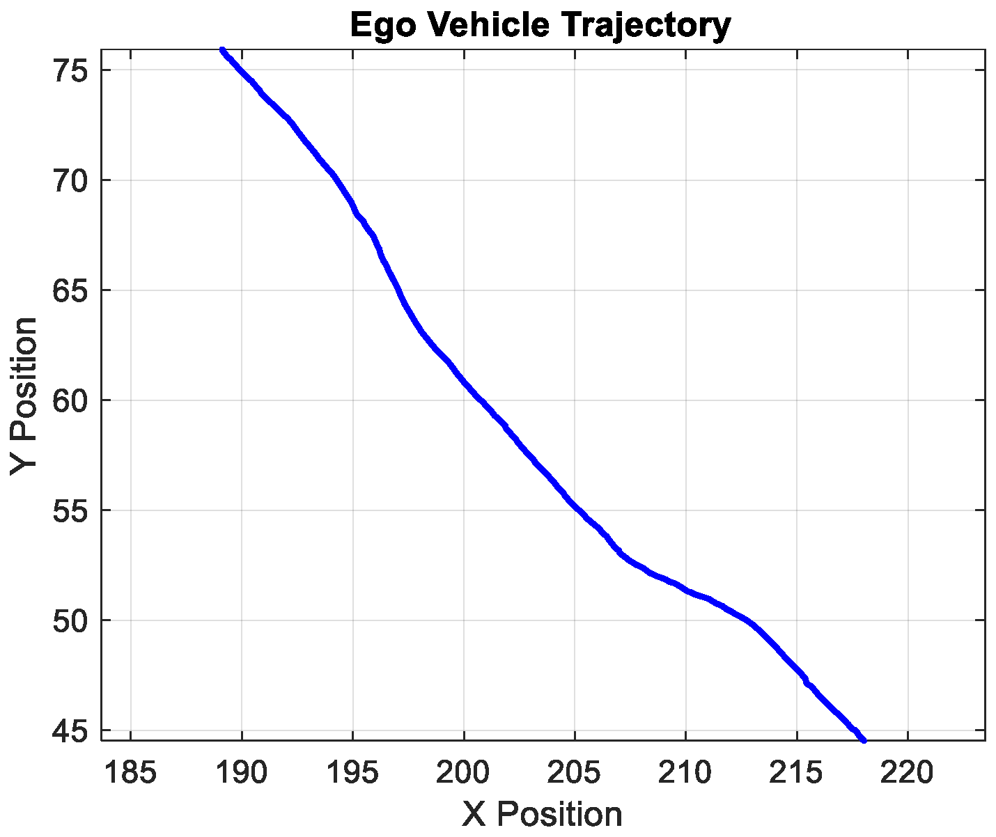
Figure 1. Our framework providing a visual representation of the steps involved in the classification of tracks, allowing the generation of interaction dictionaries and the localization through the MJPF.
Applsci 15 05181 g001
Figure 2. Ego vehicle trajectory.
Applsci 15 05181 g002
Figure 3. Track positions relative to ego vehicle.
Applsci 15 05181 g003
Figure 4. Clustering results for the generalized states of the seven tracks and the ego vehicle.
Applsci 15 05181 g004aApplsci 15 05181 g004b
Figure 5. DBN model during training.
Applsci 15 05181 g005
Figure 6. DBN model during the testing phase with separate track predictions.
Applsci 15 05181 g006
Figure 7. DBN structure during the training phase. Odometry sensor data and LiDAR observations are used to classify and learn tracks.
Applsci 15 05181 g007
Figure 8. DBN structure during the testing phase. Only LiDAR observations are used to match tracks and estimate ego vehicle positions.
Applsci 15 05181 g008
Figure 9. Timeline of ego vehicle interactions with clustered tracks across 393 frames. Each colored line corresponds to a GNG-clustered track ID. This interaction window supports downstream classification and trajectory modeling.
Applsci 15 05181 g009
Figure 10. Histogram of relative velocities between the ego vehicle and track clusters. A threshold at μ + σ is applied to separate dynamic tracks (in red) from static ones (in blue).
Applsci 15 05181 g010
Figure 11. Classification result based on the μ + σ velocity threshold. Blue tracks are labeled static; red tracks are dynamic.
Applsci 15 05181 g011
Figure 12. Confusion matrix for classification.
Applsci 15 05181 g012
Figure 13. Localization result of comparing the predicted ego vehicle trajectory (red) with the ground truth (blue).
Applsci 15 05181 g013
Figure 14. Localization result of showing various scenarios in different colors.
Applsci 15 05181 g014
Figure 15. Transition matrix considering different states.
Applsci 15 05181 g015
Figure 16. Continuous states anomalies over time.
Applsci 15 05181 g016
Figure 17. Discrete states anomalies over time.
Applsci 15 05181 g017
Figure 18. Box plot of continuous anomalies.
Applsci 15 05181 g018
Figure 19. Box plot of discrete anomalies.
Applsci 15 05181 g019
Table 1. Example of interaction data between the ego vehicle and Track 14. Each row represents a frame-level observation, including time, cluster indices, interaction label, and ego vehicle position.
Time (s)Track ClusterLabelEgo ClusterEgo x Position (m)Ego y Position (m)
0.1000400218.002144.5398
0.2000400218.005144.5382
0.3000400218.009244.5362
0.4000400218.001344.5405
0.5000400217.997444.5423
0.6000400217.994244.5441
0.7000400217.989344.5475
0.8000400217.988144.5494
0.9000400217.987544.5504
1.0000415217.988744.5512
Table 2. Steps followed to construct the interaction dictionary between the ego vehicle and the observed tracks. Each step transforms raw frame-level data into structured interaction entries.
StepDescription
1Temporal Alignment: Synchronize LiDAR and odometry timestamps to associate ego and track observations frame-wise.
2Track Association: Identify active TrackIDs using the JPDA filter at each frame.
3Cluster Assignment: Assign ego and track positions to their respective GNG clusters to extract cluster indices.
4Interaction Labeling: If ego and track positions fall within a defined spatial proximity, label the interaction as L = 1 ; otherwise L = 0 .
5Dictionary Population: Store the interaction entry as I = { t , C ego , C track , L , x , y } , where ( x , y ) is the ego vehicle position.
Table 3. Parameter settings used in the JPDA tracker and GNG clustering algorithm. All values were empirically tuned using the training dataset.
ModuleParameterDescription and Value
JPDA TrackerGating threshold0.8 (based on Mahalanobis distance)
Confirmation count3 consecutive detections required
Missed detection toleranceUp to 5 missed updates allowed
GNG ClusteringMaximum number of nodes100 (adaptive per trajectory length)
Learning rate (winner) ϵ b 0.05
Learning rate (neighbor) ϵ n 0.0006
Maximum edge age50 iterations
Node insertion intervalEvery 100 steps
Error decay factor β 0.0005
Table 4. Performance metrics of the classification module on iCAB and KITTI datasets.
MetriciCABKITTI
Accuracy87%82%
Precision88%80%
Recall94%89%
F1 Score91%85%
Table 5. Ablation study results showing mean localization error (in meters) for different configurations of the framework.
MethodMean Error (m)
Full Framework (MJPF + Combined Dictionary)0.17
Without Combined Dictionary (Single Track Only)0.23
Without MJPF (Kalman Only)0.29
Without Dictionary (Odometry Only, No LiDAR)0.36
Disclaimer/Publisher’s Note: The statements, opinions and data contained in all publications are solely those of the individual author(s) and contributor(s) and not of MDPI and/or the editor(s). MDPI and/or the editor(s) disclaim responsibility for any injury to people or property resulting from any ideas, methods, instructions or products referred to in the content.

