Three-Dimensional Visualization of Articulated Mechanisms: Coupling of Their Dynamic and Virtual Models Using the Example of Driving of the Omnidirectional Mobile Robot

Abstract

This paper proposes a novel approach to the virtual 3D modeling of articulated mechanisms. It follows the widespread use of XML (eXtensible Markup Language) for various applications and defines a version of XML that is specially designed for the description of 3D geometric models of articulated bodies. In addition, it shows how the 3D geometric model of a mechanism can be gradually developed through the use of suitably defined elements and stored in a corresponding XML file. The developed XML model is processed, and using a powerful VTK (Visualization Toolkit) library, the corresponding virtual model is built and shown on the computer screen. To drive the virtual model, the dynamic model of the mechanism is developed using Bond Graph modeling techniques. Virtual 3D geometric and dynamic models are created using the corresponding software packages: BonSim3D 2023 Visual and BondSim 2023. The models are interconnected by a two-way named pipe. During the simulation of the dynamic model, the parameters necessary to drive the virtual model (e.g., the joint displacements) are collected and sent to the virtual model over the pipe. When the virtual model receives a package, the computer screen is updated by showing the new state of the mechanism. The approach is demonstrated using the example of a holonomic omnidirectional mobile robot.

1. Introduction

With the development of 3D CAD technologies, the visualization of processes and systems has become a powerful method and has been increasingly used in the processing of new products and process design, providing numerous benefits, such as a shorter development time and lower costs, the possibility of testing and verifying functionality before a product’s production, the ability to check possible part collisions in space, the ability to compare different product and process solutions to choose an optimal one, etc.

The idea of gaining remote access to the information of automatic systems and their visual representation appeared with the invention of the Internet. In [1], online approaches are proposed for the remote control of automatic systems based on synchronous and asynchronous capabilities to control the developed 3D models using XML (eXtensible Markup Language) technology. Many researchers have developed simulators with visual programming environments for the education, development, validation, and optimization of various products and processes. To simulate both industrial automation and embedded control systems in a 3D environment, many software have been developed and widely used, including the following: Factory I/O (by Real Games) for industrial automation training and factory process simulation; Siemens Tecnomatix Plant Simulation for large-scale factory and industrial system modeling; Automation Studio (by Famic Technologies) for hydraulic, pneumatic, and PLC-based automation; etc. Simulators have been used as effective tools in numerous studies for optimizing energy consumption [2] and controlling noise due to flights of unmanned aerial vehicles systems, such as drones [3]. A very important area of the application of simulators is in the educational process, where, without the need for access to real physical equipment, one can master their operation, and they are widely used in educational processes in various fields, including medicine [4,5,6], aviation as flight simulators [7,8,9], and STEM education [10]. In order to improve microcontroller-based education, a 3D virtual factory simulator was proposed in [11], as well as Tinkercad (from Autodesk), Proteus (from Labcenter Electronics), and many others. A systematic review of driving simulator validations is provided in [12] in the context of educational robotics [13], training simulators for manufacturing processes [14], body measurement technology in digital skiing [15], and many others.

The popularity of XML-based languages has increased in recent years due to the possibility of exchanging data between heterogeneous systems, and they have been addressed in numerous studies, including the following: XML-based Robot Description Language for describing robot structures was presented in [16]; RoboML based on XLM for robot programming in [17]; AVSML (Agent and Virtual Space Markup Language), an XML-based markup language for integrating web information into virtual 3D space in [18].

In [19], an application for the robot palletizing process was developed in the ABB native language RAPID, with an interface written in XML that has the ability to work together with the software for offline robot programming RobotStudio.

An XML was used as the basis for a new language to specify a video game—Video Game Description Language (XVGDL) [20].

One of the most common robot description formats—Unified Robot Description Format (URDF)—was introduced in 2009 [21,22] with the development of an open-source set of software libraries and tools for building robot applications, named the Robot Operation System (ROS). URDF is based on XML technology and was applied to describe the kinematic structures of robots, their dynamics, and geometry [22,23]. The self-calibration procedure of a low-cost five-axis 3D printer, where calibration data were used to generate a kinematic model in URDF format, was proposed in [24]. Procedures for the automatic generation of URDF files from Solid Works are the subject of research in [25,26], for the visualization of a modular robot manipulator in [25], and a micro-assembly robot in [26].

Similarly to URDF, the XML-based Simulation Description Format (SDF) has emerged, expanding the possibilities of developing a robotic environment [23]. Because both URDF and SDF are XML-based, they follow the rules of XML syntax, making them both human-readable and machine-parsable. SDF was used to describe Building Information Modeling objects and has been integrated with the finite element method (FEM) and ROS to assess structural stability [27].

An overview of robot description formats and methodologies for visualizing robots and their environment is presented in [28].

The visualization of systems and devices, i.e., their virtual 3D models and digital twins (DTs), is recognized as a potential solution for the improvement of these processes and systems and therefore attracts extreme attention from the academic community and industry. An XML is one of the most commonly used technologies to develop a digital twin. In [29], due to the analysis of the sheet metal punching process, different configurations of sheet metal punching machines were developed with a complete virtual 3D scene in the form of XML files. In the example of a digital twin of the overhead crane [30], a system framework is presented for its integration into an Extended Reality (XR). The application of digital twins as possible answers to the challenges in production systems is the subject of research in [31,32]. In [31], an overview of the possibility of digital twins to support the Human–Robot Collaboration in production systems is presented, as well as a comparison of key commercial software regarding the possibility of fulfilling the requirements for DT development. The review of research in [32] pointed out numerous gaps in the application of DT in production systems, as well as indicated directions for future research.

As robotic systems become increasingly complex, the role of simulators has become highly important in robotics; this is due to the numerous built-in sensors that robots possess and the complex tasks they have to perform. The design, analysis, and performance optimization of robots, as well as their navigation of unstructured environments, can be significantly simplified by using software for modeling and visualization.

In recent decades, many researchers have developed different software packages for simulating and visualizing robot applications; these have grown in popularity and play important roles in solving engineering problems. Some of the simulators commonly used for the development of mobile robot applications are Gazebo [33,34], which is based on a Robot Operating System (ROS) [35,36]; Rviz, 3D visualization tools for ROS [37]; Webots [38,39]; MORSE [40]; CoppeliaSim [41,42]; CARLA [43]; Raisim [44]; MARS (Multi-Agent Robot Simulator, developed in MATLAB) [45]; CARMEN (the Carnegie Mellon Navigation Toolkit) [46]; and MoveIt [47].

To enable the right simulator to be chosen for the development of a specific robotic application, many researchers have conducted overviews of the most widely used 3D robotic simulators and evaluated their properties [48,49,50,51,52]. The authors of [53] present a comparative study of Gazebo and Unity 3D in the development of a virtual model of the collaborative robot UR3 and its application for assembly work in production. Some authors suggest use of virtual reality (VR) [54], augmented reality (AR) [55], and mixed reality (MR) [56] as powerful tools for the modeling and visualization of complex systems. Some useful algorithms for the modeling and visualization of robots in MATLAB are presented in [57]. Generally, the popularity of mobile robots has grown significantly in recent years, attracting scholarly attention around the world.

This study proposes a novel approach for the 3D geometric modeling of articulated mechanisms, based on the BondSim3DVisual version of XML [58]. Two-way communication between the two models was established using named pipe technology.

The proposed approach is applied using the example of the mobile robot FESTO Robotino [59]. The basic premise is to provide a connection between the developed virtual model and its dynamic model, created using another software package [60]. FESTO Robotino is complex enough to be chosen as a representative example. It is characterized by excellent maneuverability, which is achieved using three omnidirectional wheels. As such, it is the subject of many analyses [61,62,63,64,65,66,67,68]. Generally, the design and development of omnidirectional wheels have also received a good deal of scholarly attention [69,70,71,72].

The dynamic models for various mobile robots were developed several decades ago, but, due to the complexity of omnidirectional wheels [63,64,65,66,67], the attention of researchers around the world is still focused on dynamic modeling and the design of an appropriate control algorithm for the navigation of mobile robots that are equipped with such wheels [73,74,75].

In our study, we analyzed the lateral rolling of the rollers that comprise the wheels. A dynamic model, based on the concept of the component model approach, was created using the bond graph technique in BondSim [60,76].

The virtual 3D model of Robotino presented here was developed using an XML approach in the BondSim3DVisual application. The methodology for the development of the virtual model presented here is an updated, modified version of the method presented in [77]. The proposed markup language is a simplification of the general XML scheme found elsewhere [58], and it serves as a replacement of a C-type language introduced in BondSim3DVisual [60]. The proposed version was designed for the 3D geometric modeling of articulated bodies, such as robots, multi-finger robot hands, mobile robots, multi-leg platforms, cranes, and similar objects. Using a DOM (document object model)-like approach, an XML document can be represented as a tree of elements. Thus, the structure of the 3D geometric model of an articulated mechanism can be represented as a tree of constitutive elements and attributes in the computer memory. The virtual 3D model is generated from an XML tree using the powerful VTK library [78,79,80].

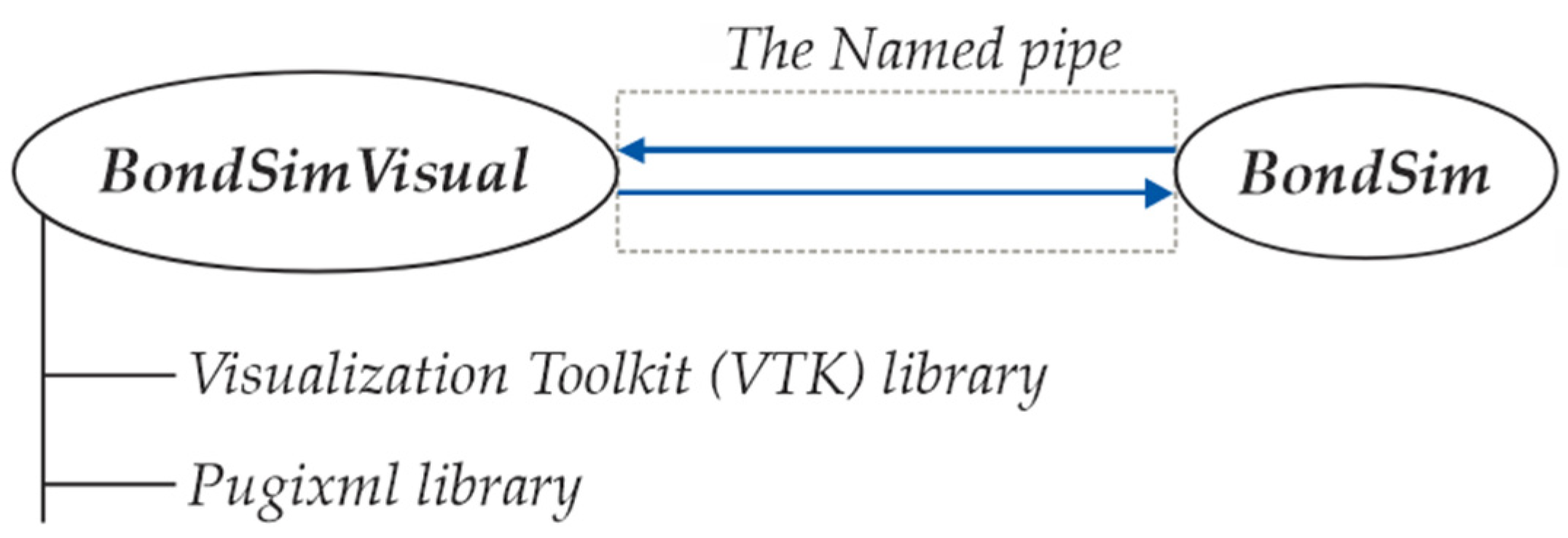
Between these two processes—the virtual, which works in the BondSim3DVisual environment, and the dynamic simulation, which runs in the background of BondSim—there exists a two-way communication based on named pipe techniques. After validation in a virtual environment, the proposed algorithms can be applied to a real robot. Verification of the robot’s behavior in a virtual scene reduces the need for extensive experimental work with real robots.

FESTO implements a similar idea for Robotino using two software packages: RobotinoView for driving Robotino and RobotinoSim to visualize a workplace using Robotino [81,82]. The approach presented here is more general and refers to the development of dynamic and virtual 3D models for any articulated mechanism, not only Robotino. Such models can exchange information with each other in planned future research on real physical systems according to the concept of digital twins.

The rest of this article is organized as follows. The methodology for developing a virtual 3D model of an articulated mechanism is described in Section 2. The dynamic model of Robotino, developed using bond graphs, is presented in Section 3. The simulation results are presented in Section 4. Finally, we offer some concluding considerations and propose directions for future work.

2. Virtual 3D Modeling of Articulated Mechanisms

2.1. The Basic Approach

Visualization in 3D space provides a representation of three-dimensional objects on a computer screen, similarly to how they are seen in the real world. In the real scene, we have several essential items (Figure 1):

• Three-dimensional space with objects in it;
• Sources of the light, such as the sun or light bulbs, which illuminate the scene;
• A person looking at the scene.

Generally, the objects are not static but move around the scene, e.g., a robot hand moves over the scene to grasp a part and moves it to another object to place or insert it there. We analyze their motion in the world space OXYZ. We assume that the XY plane is where the objects lie, and we track them along the negative Z-axis.

To visualize the objects and their movement around the scene, we follow these steps:

• Generate virtual 3D representations of them as 3D geometric objects;
• Generate a dynamic model of the entire system in order to simulate the objects’ motion;
• Interconnect these two worlds, 3D geometric and dynamical, by suitable means to enable interactions between them.

To achieve this, we use two applications, which were developed specifically for this purpose: BondSim3DVisual and BondSim [76], as shown in Figure 2.

2.2. Generating the Virtual 3D Model

To generate a virtual 3D model of an articulated mechanism, the BondSim3DVisual application was developed using the Microsoft Visual C++ language. It is used for the construction of the virtual 3D model of a mechanism and its generation on the computer screen. It uses a special version of Extensible Markup Language (XML). The application uses the well-known pugixml library [83] to support the processing of XML code.

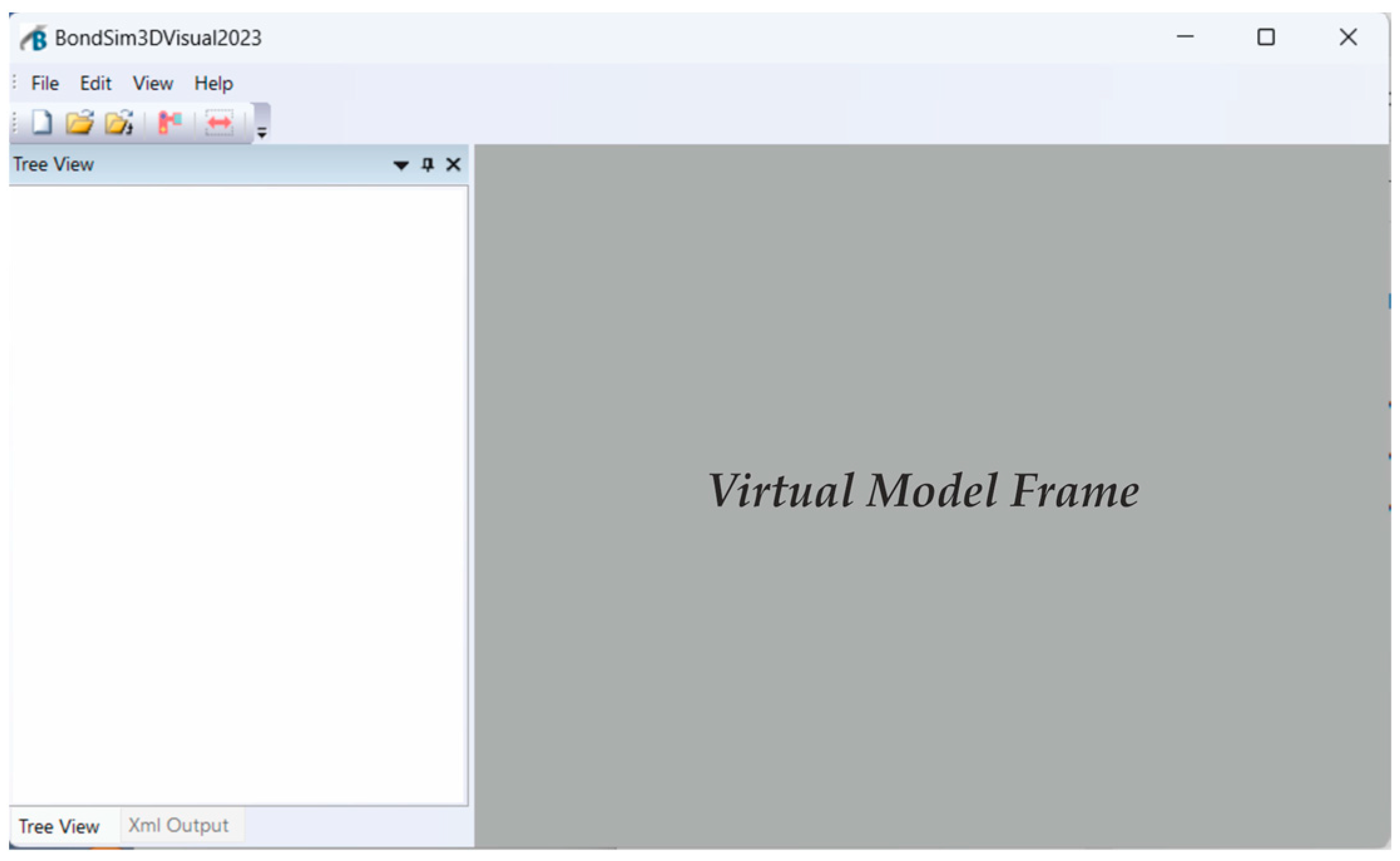
Upon opening the application, an empty mainframe appears, as shown in Figure 3. It is divided into two parts. On the left side there are two tabbed windows: Tree View and XML Output. The first one enables the construction of the Document Object Model (DOM)-like XML model tree. Thus, the model is not developed as a conventional XML document, but as a DOM-like tree. It starts at a root, and suitable elements and attributes are inserted one after another other as its branches or leaves. Simultaneously, a corresponding XML document is generated in a read-only XML Output window. To see it, we simply click its title (Figure 3). The right side of the program frame is used to create a document window containing the virtual 3D objects corresponding to the XML model on the left.

The approach that we use is general purpose and can be applied to different articulated mechanisms, not only Robotino. The building of the XML model starts at a root and continues by adding different elements, with its attributes systematically following the structure of the real equipment. To this end, a wide range of XML elements are available, ranging from simple geometrical shapes, such as cuboids, cylinders, spheres, bodies of revolution, and CAD-designed parts, to joints for interconnecting bodies, as well as different types of transformers, which are used to transform XML element body models between different coordinate systems and driver units. In this way, a virtual model is obtained, which has an appearance and structure very like the modeled equipment.

There is no restriction on the number of pieces of equipment that the working space can contain. As such, a project root is used, in which we may insert different items from the application database (XML models of robots, humanoids, transport systems, and others). However, as the population of the working scene increases, more computer resources are needed in order to efficiently update the computer screen.

The problems addressed using this application are divided into several groups: projects, robots, tools, and objects. This division is rather arbitrary and serves to define the roots of the model trees and the directories where their XML documents are stored. The models are stored as XML files, i.e., text files with the extension XML.

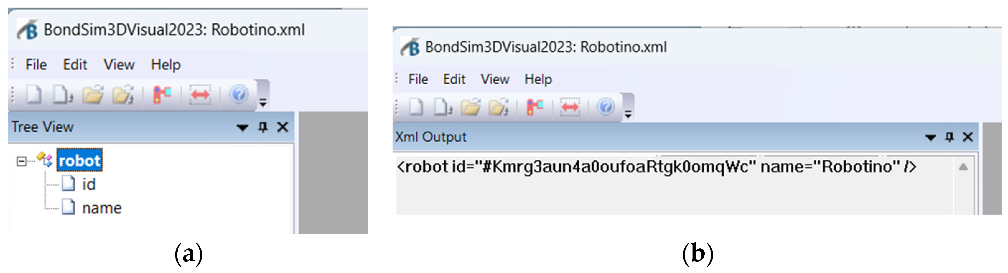
From a modeling and visualization point of view, robots, tools, and objects are all treated in the same way. Thus, when we need to develop a new robot model, e.g., a 3D model of Robotino using the BondSim3DVisual application, we need to assign a unique name to the model, which is used as the filename for storing the generated XML document in the robot directory. We may select simply Robotino as the file name. The program starts by creating the robot tree root and adding the attributes as children (Figure 4a). The attribute id represents the robot identifier. It is a machine-generated unique string of letters and numbers, as shown in Figure 4b. The name attribute contains Robotino’s textual value.

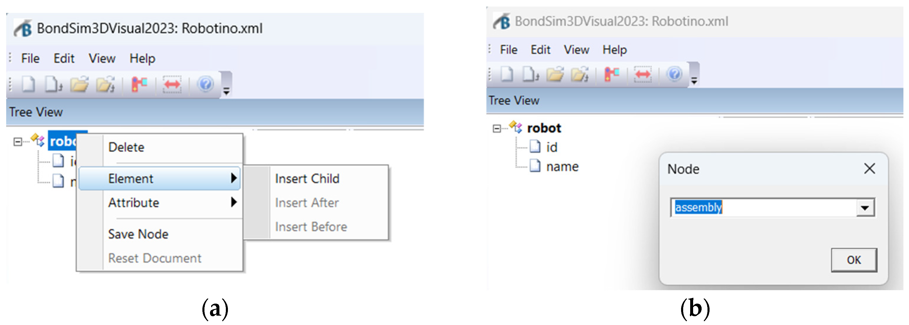
The operations on the tree are very simple. Starting from the root, we insert elements or attributes by selecting a corresponding node (an element or attribute) by clicking it with the mouse and applying the edit menu command, or by right-clicking it with the mouse, upon which a drop-down menu appears, from which an element or attribute can be chosen (Figure 5a) for insertion. Another drop-down menu now appears, from which a suitable command can be selected, either to insert a new item as a child, or above or below the selected item. The menu disappears, and a dialog window appears, from which an element or attribute node can be selected (Figure 5b). After selecting and clicking OK, the dialog window closes, and the selected item appears in the tree. The structure of the virtual model is generated systematically, starting at the robot root and with its branches (elements) and leaves (attributes) hierarchically added following the structure of the mechanism being modeled.

Generating the scene on the computer display is the responsibility of the computer graphic subsystem, which consists of display hardware, graphics hardware, and a graphics library. It is possible to program the graphic subsystem directly by use of corresponding languages, such as OpenGL, DirectX, etc. However, many applications use a suitable application library to simplify this task. To that end, the BondSim3DVisual tool uses VTK, a powerful C++ library [78,79,80].

By applying the Create 3D Scene command, the XML model description is processed, and the corresponding virtual model frame is created on the right side of the application’s frame windows (Figure 3).

2.3. Modeling the Articulated Mechanism

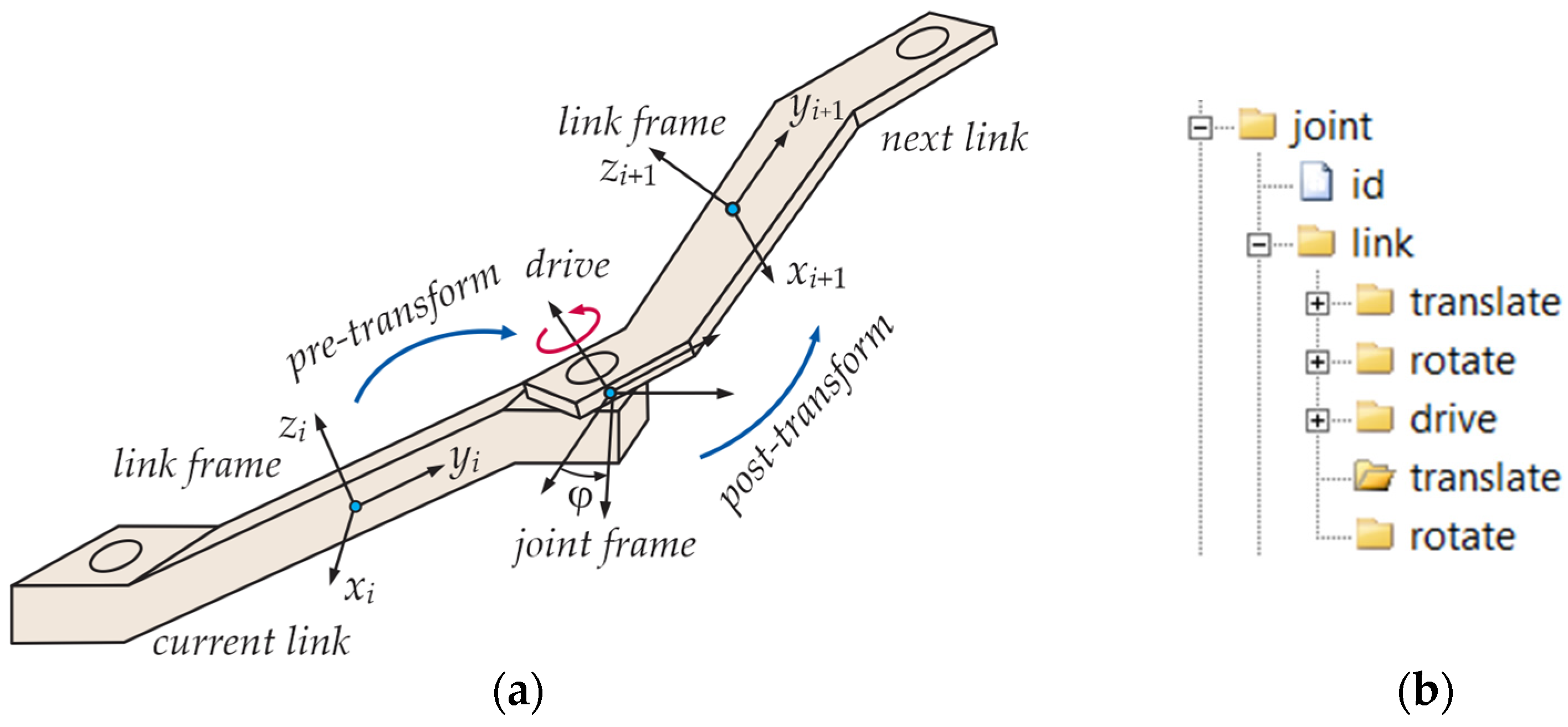
A typical articulated mechanism consists of a base (link 0) and a series of body links connected by joints. To describe this mechanism, we use different coordinate frames. Thus, every body links to an orthogonal coordinate system, which is fixed to the particular body link. There are two coordinate systems associated with every joint, which have common origins. One of these frames is fixed to the previous link, and the other to the next link (Figure 6a). The relative position of these frames can be described using a common joint axis and a rotation angle/translational displacement, by which one joint frame is displaced with respect to the other.

Figure 6a shows the simple case of a revolute joint. To define the next link coordinate frame defined by the corresponding rotation matrix, we start from the current frame rotation matrix and use pre-transforms to transform it to overlap with the current joint frame fixed to the current link. These transforms usually consist of translations that move the origin of the current link frame to the origin of the joint frames and the rotation of the translated frames to align with the joint frame, which is fixed to the current frame. Next, a drive transform is applied; this typically consists of the rotation or translation of the other joint frame around/along the joint axis. Finally, we apply the post-transform, which aligns the other joint frame with the next link body frame. These transforms can be succinctly described by the XML tree segment shown in Figure 6b.

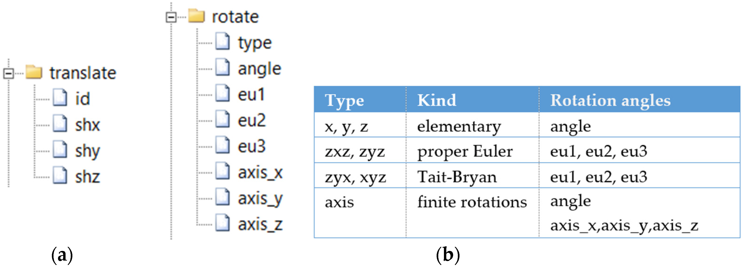
Figure 7 depicts the translation and rotation elements. They are used in Figure 6b to transform the previous link frame to the drive element, and produce drive elements for the next link frames. Often, transforms along the body links are much simpler. Thus, a joint coordinate frame fixed to the previous link can be used simultaneously as the link frame. In this case, pre- and/or post-transforms are not necessary (they are identity transforms); only the drive transform is needed.

The <drive/> element represents the link driver, which can be real or virtual. In any case, it is defined by the type attribute, which can be one of the following driver types: prismatic_x, prismatic_y, prismatic_z, revolute_x, revolute_y, revolute_z, or spherical. The first six types correspond to joints with a single degree of freedom, and the last refers to rotation with three degrees of freedom about an axis through the center of the joint.

After the rotation matrix of the next link frame is defined by the above transforms, we need to describe the geometry of the next link. We may use different geometric elements such as cuboids, cones, cylinders, and bodies of revolution for this purpose. All such elements are the children of the next joint, and thus they use as the reference frame the frame of the next body link, the id of which is defined by the link element in Figure 6b. Hence, all of these elements have to follow the link element. All of these elements have a unique id attribute, which is used to refer to them.

There is a special element known as assembly. The geometric elements are added to it by referring to them by their ids. In this way, all of the subsequent body link geometric elements can be referred to as units according to the assembly id attribute. We can also use it to transform the position and orientation of the added elements with regard to the reference frame.

The articulated mechanism’s parts typically have complex shapes and are usually generated using 3D CAD software (e.g., SolidWorks, Catia, etc.) [84], from which they can be exported in the form of STL files. This is the case with many robots, including the Robotino. In this way, the virtual 3D models of such robots can be reconstructed so that they are very close to the real devices. The main difference is in the color of the robot’s parts, because they are not defined in STL files, which contain only the geometric data. The corresponding stl files are specified by the part elements.

The final element in the joint segment is the render element. The element is inserted at the same level but below all of the body elements or assemblies it refers to. It connects the geometry of the element or assemblies it refers to with the visualization object (the actor). It also connects to the link frame (the next body frame). Because the geometry does not contain information about color, it is defined here. The color can be defined by a name, as in web browsers (Edge, Google. etc.), or according to the red, green, or blue (RGB) color indices in the range 0.0–1.0. This value is set to the color of the current visualization object.

2.4. Modeling of FESTO’s Omnidirectional Mobile Robot Robotino

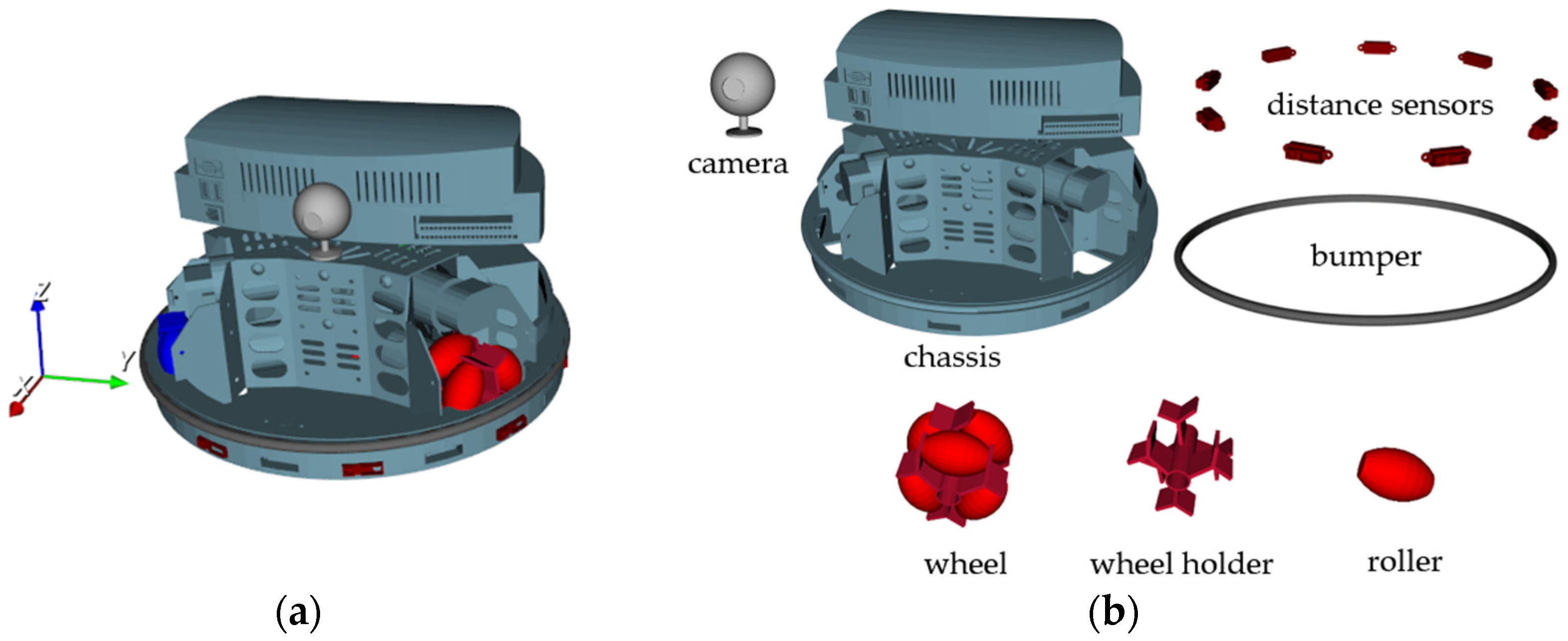
The Robotino is an omnidirectional device, which has the ability to move over the ground in any direction, regardless of the current orientation of its wheels (Figure 8). This is mainly a result of the special design of the wheels. For the version of Robotino studied here, every wheel consists of two groups of three rollers each, which are contained in a wheel holder (supporter), in which they can rotate. The rollers in one group, e.g., the front or back group, are angularly displaced by 60° with respect to the other in such a way that, when looking at the wheel’s outer circle at the point of contact with the ground, the end of a roller in the first group overlaps with the start of the roller in the other group. In this way, during the rotation of a wheel, one roller is always in contact with the floor and rolls over it. The coordinate system shown in Figure 8a is the world coordinate system with which the device is described. It is displaced in order not to overlap with the device. The Robotino consists of a chassis and three wheels, which are displaced around the vertical axis by 120°. The wheels are driven by DC motors, which are connected to wheel axles by toothed belts and planetary gears. The basic parts of Robotino are shown in Figure 8b.

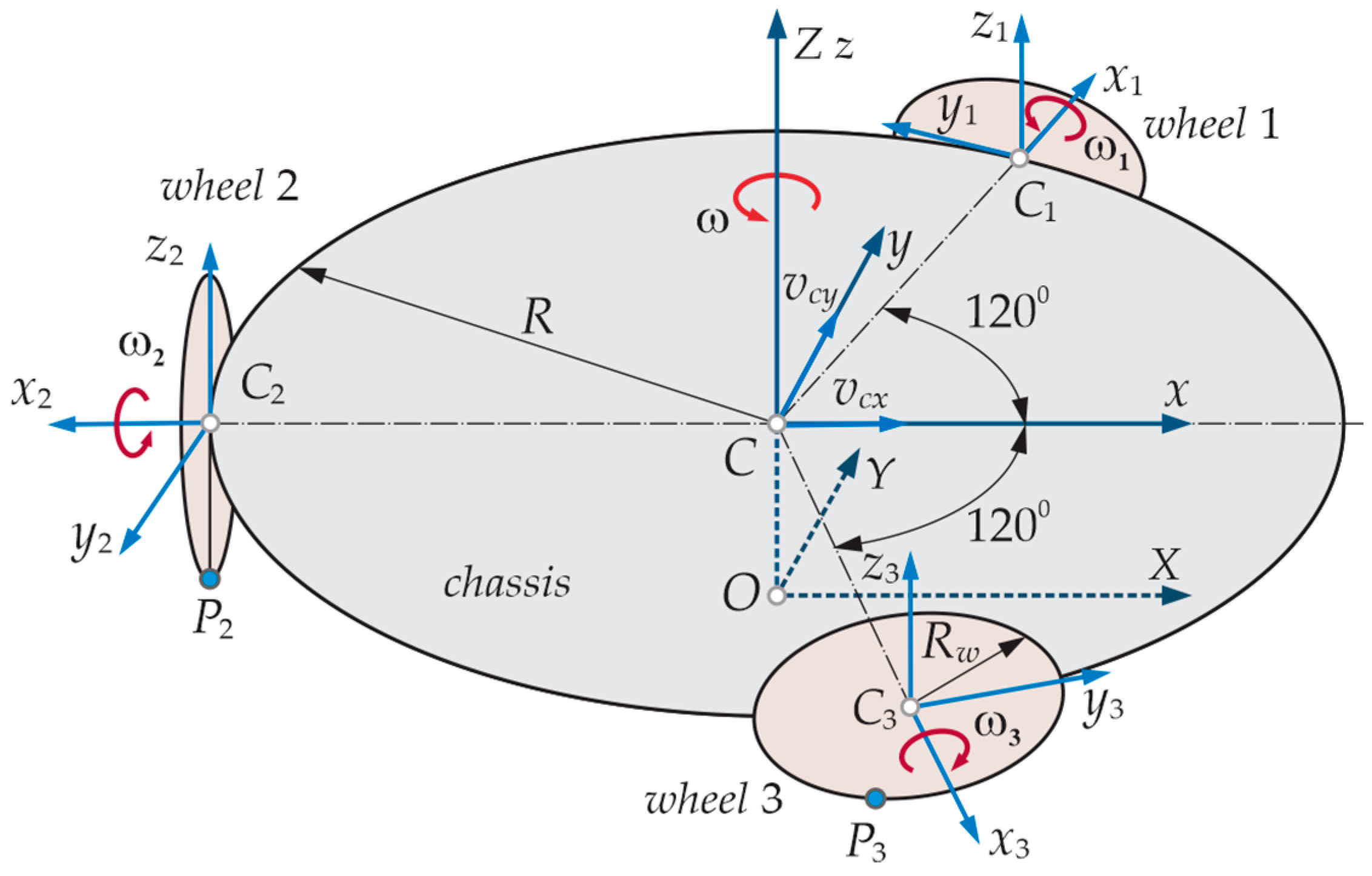
Figure 9 shows a scheme of Robotino with the local coordinate frames defined. There are three frames with the origins at the wheel centers C_i (i = 1, 2, 3) and whose x_i-axes (i = 1, 2, 3) are directed along the wheel rotation axes. We also added another local frame whose x-axis is directed opposite to the x₂-axis and serves to orient the Robotino. Their z_i- and z-axes are parallel with the world’s Z-axis; the y_i- and y-axes are created by rotating the x_i- and x-axes around the z_i- and z-axes by 90° in a positive (counterclockwise (CCW)) direction. The local coordinate frames are fixed to the Robotino’s chassis and move jointly with it. We created a new virtual model of the Robotino, as explained in Section 2.2 (Figure 4). It generates the corresponding robot root (Figure 10a).

Next, to enable the robot to be moved over the world frame, we inserted three virtual joints. The first one is inserted as the child of the root and the other two as the children of the previous ones. The joints have link elements containing only the simple drivers—the first is the prismatic one along the X-axis, the next is the prismatic one along the Y-axis, and the third is a revolute around the Z-axis. Note that these joints do not exist in the real device.

Following the last joint’s link element, the chassis, bumper, distance sensors, and camera are inserted into the tree by the part elements and by specifying their id and name attributes. Afterwards, an assembly element is inserted; it is used to properly position the part with respect to the joint reference frame. Next, a render element is added to specify the color and generate a 3D view of the part.

After all the parts’ elements are added, we add a probe. It is used to define the particular point in the robot’s structure that we wish to monitor while the Robotino’s 3D model is in motion and returns to its current coordinates. Here, we put it at the center of the base of the Robotino’s chassis. We may add some other points as well.

Finally, there are three additional joint elements in parallel (Figure 10a). They correspond to the axles on which the wheels are mounted (Figure 9). Their link children define the positions and orientations of the corresponding local frame. The object elements define the corresponding omnidirectional wheels that rotate jointly with the axles.

The model of the wheel object is generated using a method similar to that used for the robot. However, here, we use the New/Object command and set the names as follows: Wheel_1, Wheel_2, and Wheel_3. The corresponding model tree is shown in Figure 10b. The part element defines a roller supporter. It is added to the assembly element, and its position and orientation are defined there. Finally, the render element, which refers to the last assembly element, defines its color and generates a 3D view of the supporter. The next six joints correspond to the rotation axis of each of the six rollers. The structure of the joints’ tree is similar to that of the other joints. Their axes, geometric shapes, and colors are defined, and a 3D view is generated. This allows for the modeling of every roller motion separately.

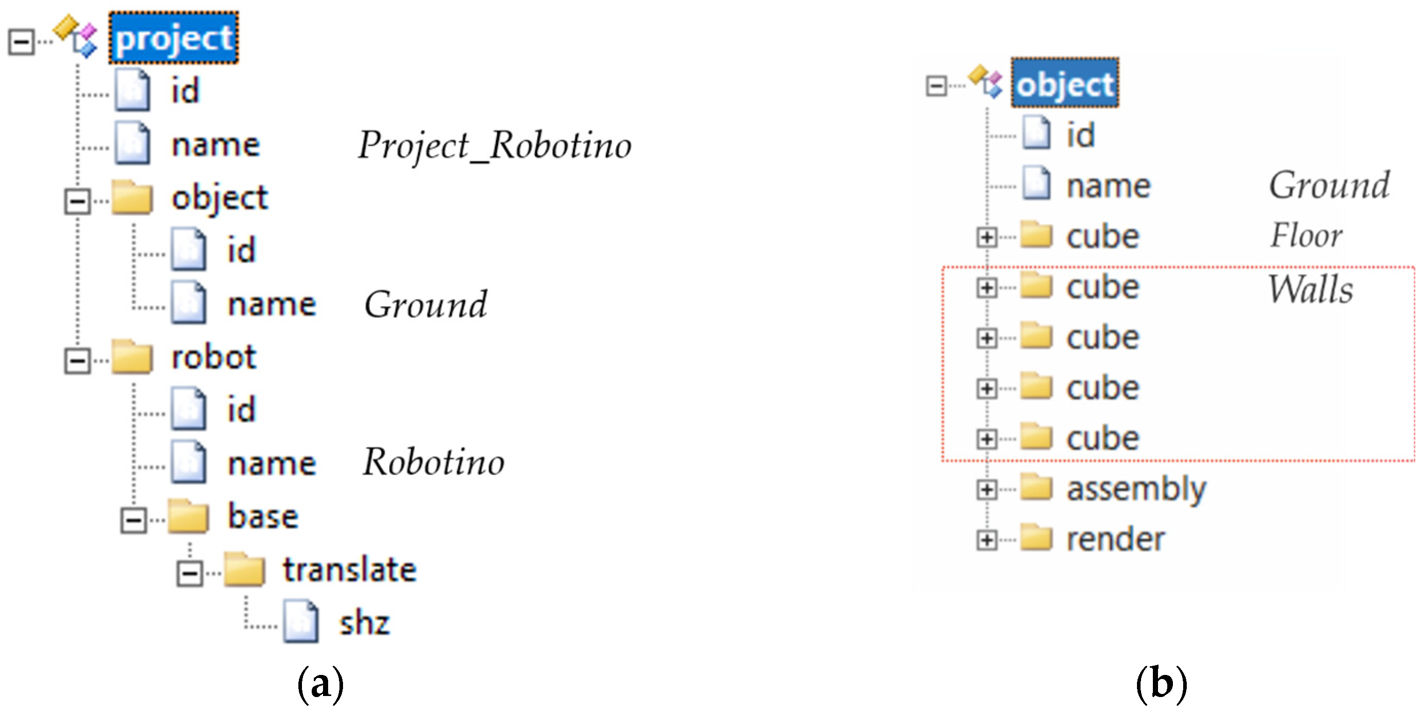
The projects are used to define the workspace where the robots, tools, and objects are used. The project shown in Figure 11a contains a Robotino robot that is moving over a ground floor constrained by walls, as described by the object element.

The XML model of the ground is shown in Figure 11b. It consists of a base floor in the form of a thin cuboid, and the walls are also cuboids. They are added into the assembly element to properly position them. The render element defines the color of the ground object and generates a 3D view of it on the screen. The robot specified is a Robotino device. It also contains the base element, which defines its position with respect to the floor. (The base of the Robotino is moved up so that the wheels just touch the ground.)

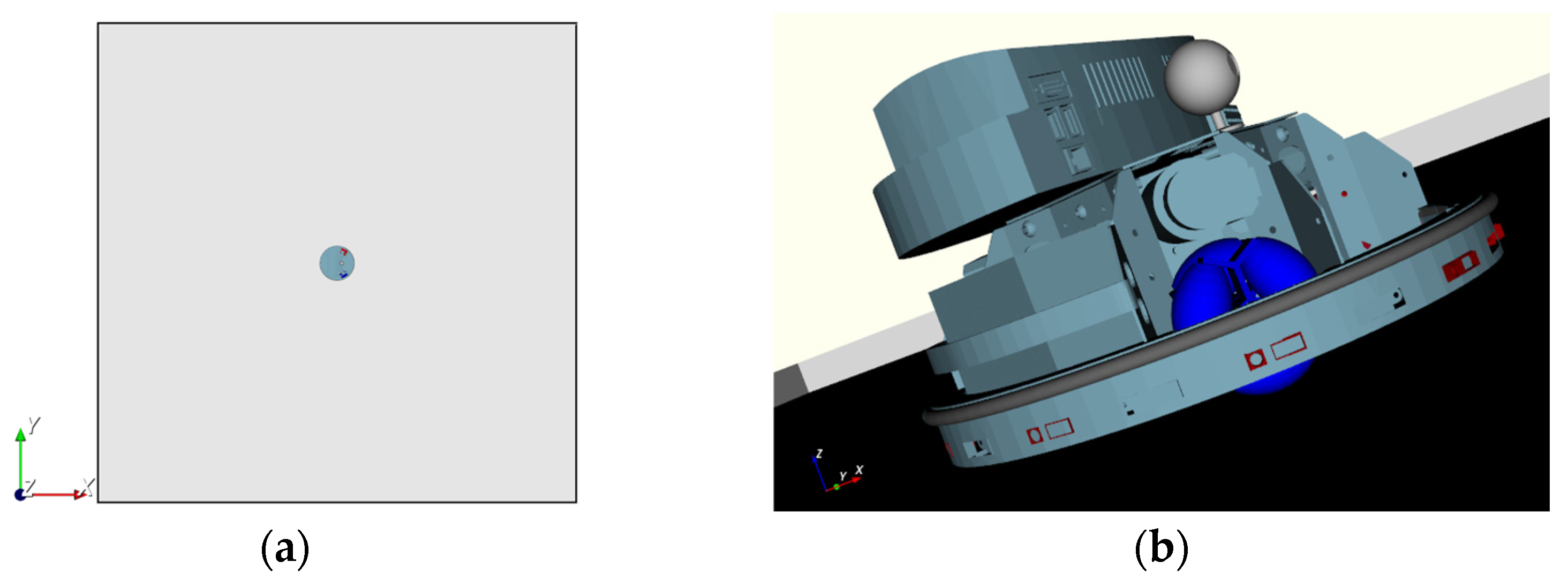
After the complete XML model of the Robotino project has been developed, we begin processing it in order to generate a 3D view. First, the Robotino project is opened using the Open-Project command from the File menu, and Project Robotino is selected. Next, we use the Create 3D scene command from the File menu. The processing starts from the project root. When object or robot elements are encountered, the application reads the names of the attributes and finds the corresponding XML files, loads them, and continues processing from their roots until all processing is complete. Figure 12a shows the scene generated. To better show the generated Robotino device and the ground, the view direction of the scene is modified by pressing the cursor on the screen near the device and dragging it, and then sizing it up by rotating the mouse wheel (Figure 12b).

3. Development of a Dynamic Model of the Robotino with Bond Graphs

3.1. Introduction to Bond Graphs

Here, we present a short introduction to the bond graph methodology, following [76]. Bond graphs were introduced by Prof. Henry Paynter (M.I.T.) in 1959. Since then, many researchers have participated in their further development. In the classical formulation, they are associated with causality assignments, i.e., input–output relationships assigned to the bond graphs [85]. This procedure can generate a mathematical model of a system in the form of ordinary differential equations, which are generally relatively easy to solve. However, often, this is not the case. To simplify the problem of generating a mathematical model from bond graphs, in [76], causality assignment procedures for bond graphs were completely rejected, and the mathematical model was developed in the form of DAEs (differential algebraic equations) (see Section 3.6).

3.1.1. General Bond Graph Components

In [76], modeling with bond graphs is achieved using an object-oriented approach. Hence, every entity in the bond graphs—components, ports, bonds, etc.—is constructed from a class, which is derived from the top abstract class; they are represented on the computer screen with a graphical symbol. The general bond graph component, or word (textual) model, is shown in Figure 13. It is characterized by the name, which can be anything, e.g., wheel, and ports, which facilitate the interaction of the component with its environment. There are two types of ports: power and control ports. The first are represented by the half arrows, which indicate the assumed direction of the power transfer, i.e., into or out of the component. To every power port are assigned a pair of port variables: effort and flow.

These variables can be simple variables, e.g., a force component F_x or velocity component v_x, and they can also be more complex mathematical structures, e.g., force of velocity vectors or other mathematical entities. Their product (ordinary, scalar, or similar) is power transferred across the port into or out of the component. Transfer of power throughout a model is an essential property of bond graph models. Control signals, on the other hand, only transfer the information, e.g., the values of the angles to drive a joint. The signal port represented by an arrow direct into the component represents the component input port, and that represented by an outward-directed arrow is the output port.

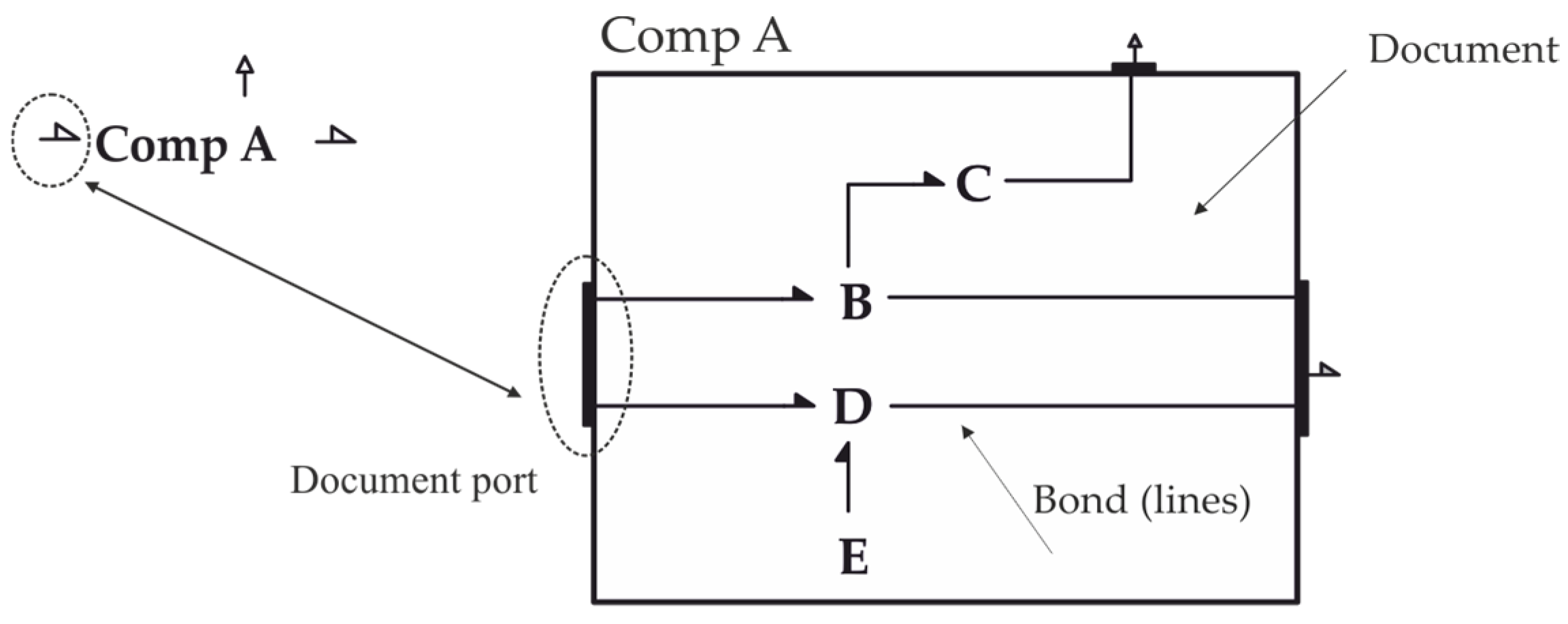
To define the model of a component, we first need to open its associated document. In BondSim, we open a component simply by double-clicking its word model (Figure 14). Note that, for every (external) component port, a corresponding document port appears in the opened document. In this way, power or information flow from outside into the component and from inside the component beyond it.

To define the model of the component, we insert into its document the corresponding word models of the physical components it consists of. These components are connected to the corresponding ports by lines known as bond lines or bonds. In this way, efforts, flows, and signals are able to move from outside into the component and further into inward components, and vice versa.

Note that the left document port is connected to two inside components, B and D, by two corresponding bonds; thus, it has two dimensions. Hence, the outside port has the same dimension: two. Thus, the effort and flow of the left power port of Comp A are vectors, whose components are corresponding efforts and flows of components B and D. It is assumed that connected bonds are ordered from the top to the bottom, or from the left to the right, of the corresponding document port. Thus, the first effort component of the left port Comp A is the effort of the left port of B, and the second component is the effort of the left port D.

3.1.2. Elementary Components

The elementary components are models of the elementary processes, i.e., the physical processes in which only one component participates. The bond graph theory defines nine such components, which are listed in

Table 1. Elementary bond graph components.

Type	Symbol	Constitutive Relation	Parameters
Inertial		$\begin{array}{l}dp/dt=e\\ p=I\cdot f\end{array}$	Inertia I
Capacitive		$\begin{array}{l}dq/dt=f\\ e=q/C\end{array}$	Capacity C
Resistive		$e=R\cdot f$	Resistance R
Transformer		$\begin{array}{l}{e}_2=k\cdot e_1\\ f_1=k\cdot f_2\end{array}$	Transformer ratio k
Gyrator		$\begin{array}{l}{e}_2=k\cdot f_1\\ e_1=k\cdot f_2\end{array}$	Gyrator ratio k
Source effort		$e=\mathsf{\Phi }\left(t,\mathrm{par}\right)$	par
Source flow		$f=\mathsf{\Phi }\left(t,\mathrm{par}\right)$	par
Effort junction		$\begin{array}{l}{e}_1-e_2+e_3=0\\ f_1=f_2=f_3=f\end{array}$
Flow junction		$\begin{array}{l}{f}_1-f_2-f_3=0\\ e_1=e_2=e_3=e\end{array}$

.

The inertial component is characterized by generalized momentum p. It corresponds to processes governed by momentum, the moment of momentum laws in mechanics, and the Faraday law in electricity. Similar to it is the capacitive element, which is the dual of the inertial element. If we substitute effort for flow, flow for effort, momentum p for charge q, and inertia I for capacitance C, we obtain the capacitive element. Despite this, both elements are retained—perhaps because it is in accordance with the theory of mechanics and electromagnetism. On the other hand, in thermodynamics, there is no counterpart to inertial processes, only to capacitive ones. In these processes, there is an accumulation of kinetic energy, i.e., the energy of motion, in the inertial elements, and of the static energy in the capacitive elements.

The dissipation of energy is described by the resistive element. The power input to this element is defined according to its constitutive relation in Table 1, determined by:

$$P=e\cdot f=R\cdot f^2,$$

Thus, if the resistance of the element is positive, there is a constant dissipation of the power flowing into the resistive element.

The transformer is an element in which there is a linear transformation between port variables. Using the constitutive relations from the table, we may evaluate the power input of the transformer as:

$$P_1=e_1\cdot f_1=e_1\cdot k\cdot f_2=e_2\cdot f_2=P_2,$$

Thus, the transformer conserves the transfer of power across the element. The same principle holds for the gyrators. We mostly use the transformer to evaluate the transformation of the component vector over different coordinate systems. We use the gyrators to model the DC motors that drive the Robotino.

The sources of efforts and flows imply certain relationships about the effort or flow at their ports, which do not depend on the other variable, i.e., the port effort does not depend on the port flow, and vice versa. Thus, these are the ideal sources. In mechanics, they are often used to imply zero velocity or force components in the specific parts of the system.

Finally, we have two junction elements. The effort junction implies that the efforts of the element ports are added, and the sum is equal to zero. The convention is that, if port power is directed into the junction, the corresponding effort gains a plus sign; otherwise, it gains a minus sign (subtracted). On the other hand, the flows of all the junction ports are mutually equal, and we may consider the effort junction to be a flow node.

The other junction, the flow junction, behaves in the opposite way to the effort junction; it is its dual. In this element, the junction ports flows are added, and their sum is equal to zero. The sign convention is the same as in the former junction. The junction ports’ efforts are equal, and thus the flow junction may be considered to be an effort node. They are often used in mechanical systems, but perhaps the most well-known applications are Kirchhoff’s voltage and current laws in electricity.

3.1.3. Control Signal Components

The bond graph components can also have control signal input/output ports, as mentioned earlier (see Figure 13). These ports serve to transmit control signals into the component and out of it. The final targets of these signals are the elementary bond graph signal discussed previously. These components can also have input or output ports, or both. Input information carried into the component can be used to generate the element’s constitutive relation, which depends on the exterior data. The output control ports serve to extract data from the component.

In this study, the most important elementary components that require the input ports are transformers, which are used for the coordinate transformation of the vector quantities. Such transforms often need angles between the coordinate axes to define the variable transformer ratio. The output ports are often used to extract the value of common efforts or flows from the flow or effort junctions.

In addition to the control ports of the elementary components, we may use also input–output signal components for further processing. Some of the most important components are shown in Figure 15. The first of these is the input generator, which, on its output port, generates a signal; this usually depends on time and certain parameters, e.g., a·sin(omega·t), where a is the amplitude, omega is the circular frequency of the signal, and t is time. The summator achieves the summation of the input signals. It is typically used in feedback control loops. The next component is a multi-input function generator. The integrator serves to integrate an input signal. For instance, if we need to evaluate the coordinates of the position of a particular part, we may pick the corresponding velocity component from, e.g., an effort junction and integrate it. Note that the bond graph is a velocity-based approach, so, if we need the positions, we must integrate the velocities. This is not a flaw in bond graphs but a characteristic of Newtonian mechanics. Newton’s laws are valid in any inertial frame of reference. Since there is no absolute frame of reference, to determine the position of an object, we must specify the coordinate system we refer to and the initial position of the object in it. The node has one input signal and many output signals, which are equal to the input, and thus allows branching of the input signal to different components.

The display component shown in Figure 15 mimics an x–y plotter. It serves to generate x–t or x–y plots of the signals fed to its input ports during the simulation. It is widely used in models. Every modeling program must have at least one of them.

The last component in Figure 15 is named IPC (inter-process communication). This component serves as an interface between the client (bond graph program) and server (virtual 3D model generator) applications (see Section 3.6). The input port serves to collect the signals, which are sent to the server by the named pipe. Similarly, the output port delivers the signals transmitted by the server back to the client.

3.1.4. Developing the Bond Graph Model

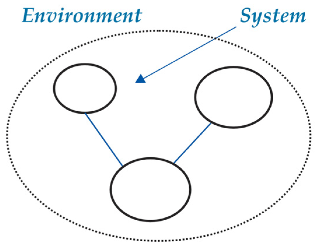
The model we are developing is, by its nature, hierarchically structured. We build it using the systematic decomposition of the objects we are modeling. We start from the basic project level, in which we can identify the basic physical components: these are subject of the project, the system, and its environment (Figure 16).

By definition, the system’s interaction with the environment is unilateral, i.e., the environment affects the system and not vice versa. Thus, the effects of the environment on the system objects are typically modeled by Effort or Flow Sources, and Input signals generators. If there is an object in the environment that is affected by the system, such an object should be extracted from the environment and added to the system.

Next, we analyze the system, identifying the main physical parts it consists of, their mutual interactions, and their interactions with the environment. In our Project Robotino, we may identify the system as consisting of four main objects: the chassis and three wheels. Its environment is the walled floor over which it rolls.

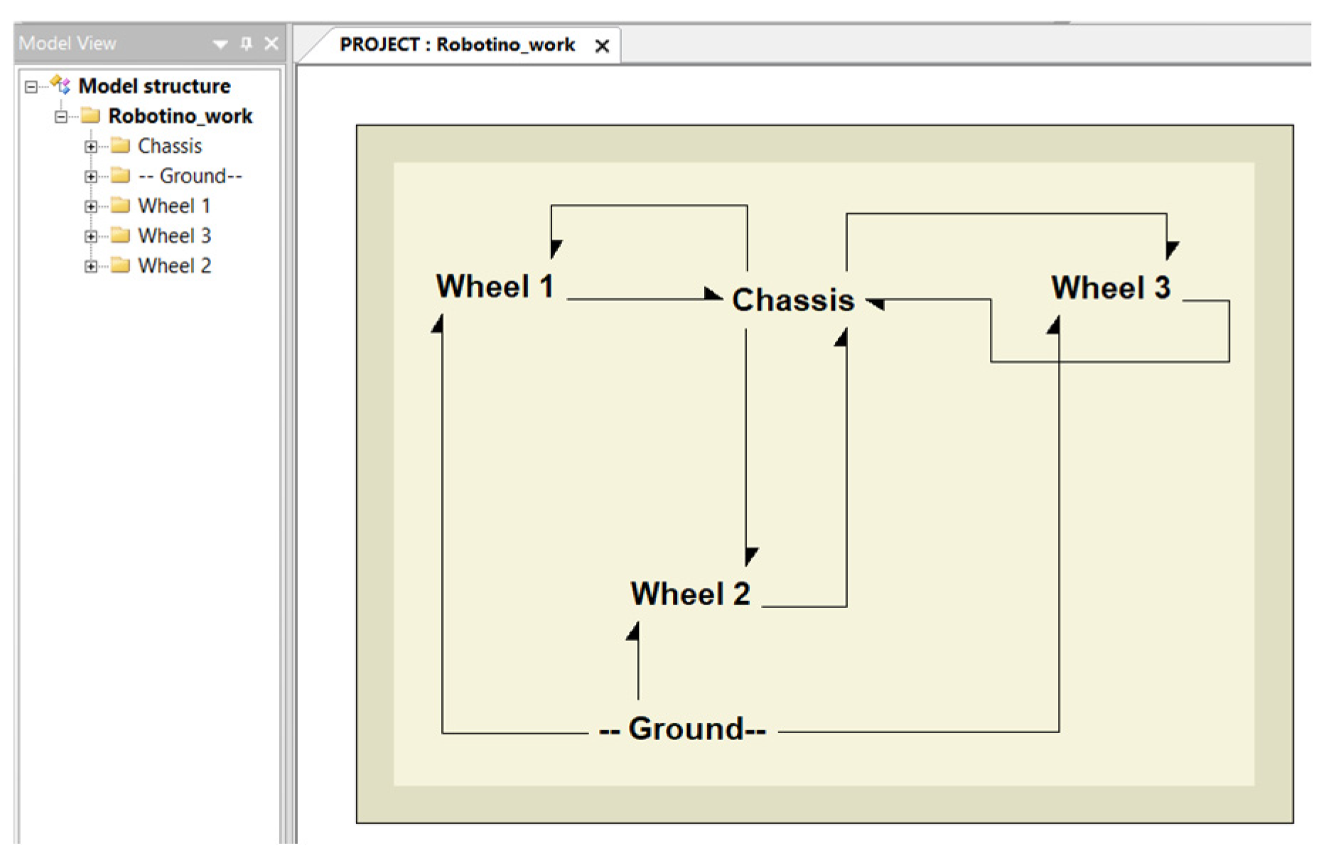
The system of the bond graph working model, which was generated using the BondSim program, is shown in Figure 17. It is a working version because some of the components the model should contain are missing, such as displays and IPC components; they will be added later. All of the main components are modeled by general (word model) components, which have corresponding name and power ports. Every wheel has three power ports. One port is connected to the corresponding port of the Ground environment by the bonds. The other one has power directed toward the chassis and is connected to it by the bond. It shows the effects of the wheels in moving the chassis. The third one, which is also connected to the chassis, shows the transfer of power from the DC motors in the chassis that drive the wheels. Note that, at the left of the Robotino’s Bond Graph model in the center of the screen, there is a tree that shows the model structure. By clicking the ‘+’ on the left of a component, we may open its internal document. Currently, there is not a document because it is not defined yet, i.e., it is empty.

3.2. Coordinate Systems

We start by analyzing the Robotino system to define the basic coordinate systems that will be used to model it.

Figure 18 shows a scheme of Robotino’s chassis—the base (see also Figure 9). There are several rigidly attached coordinate frames. Three of them are local body-fixed frames C_ix_iy_iz_i (i = 1, 2, 3), whose axes x_i are fixed and originate at the corresponding wheel centers C_i (i = 1, 2, 3). They are drawn through the base’s center C; the z_i-axes are orthogonal to the plane of motion and are directed upwards. There is another Cxyz coordinate frame whose x-axis is directed in the direction of the camera and thus shows the trajectory of the Robotino.

Hence, due to the parallelism of the z-axes, the angular velocity expressed in the world and the local coordinate frames are identical:

$${\omega }^w=\omega =\dot{\phi },$$

(1)

where the angle φ is the rotation angle of the chassis. In this study, the vectors represented in the global coordinate frame are denoted by w in the exponent. For vector components, the capital letters X and Y in the indices indicate that the components refer to the corresponding global coordinate frame. In the case of a radius vector of a point, projections onto the axis of the global coordinate frame are denoted by the capital letters X or Y, with the corresponding point indicated in the index.

The translational part of the base motion with respect to the world coordinates is described by the components of the center C velocity:

$$v_C^w=\left(\begin{array}{c}{v}_{CX}\\ v_{CY}\\ 0\end{array}\right).$$

(2)

The orientation of the local coordinate frames with respect to the world one is defined by rotation matrices:

$$R_i=\left(\begin{array}{ccc}\cos \left({\phi }_i\right)& -\sin \left({\phi }_i\right)& 0\\ \sin \left({\phi }_i\right)& \cos \left({\phi }_i\right)& 0\\ 0& 0& 1\end{array}\right), (i=1,2,3),$$

(3)

where ${\phi }_i$ is the rotation angle determined by (see Figure 18):

$${\phi }_1=\phi +\pi /3, {\phi }_2=\phi +\pi , {\phi }_3=\phi -\pi /3.$$

(4)

Thus, if the velocity vector v_i is defined in the local system, its components in the world system are defined by the transform:

$$v_i^w=R_i{v}_i,(i=1,2,3).$$

(5)

Similarly, the components of a vector, e.g., force $F_i^w$ defined in the world frame, can be expressed in the local coordinate frame by the inverse transformation matrix. Because the matrices (3) are orthogonal, their inverse matrices are simply their transpose, $R_i^{-1}=R_i^T.$ Therefore, it follows that:

$$F_i=R_i^T{F}_i^w.$$

(6)

The power defined by the scalar product of these quantities in the world system can be evaluated using the above expressions:

$${\left(F_i^w\right)}^T{v}_i^w={\left(R_i{F}_i\right)}^T{R}_i{v}_i=F_i^T{R}_i^T{R}_i{v}_i=F_i^T{v}_i,$$

(7)

Thus, it is equal to the power evaluated by the local representation of these variables. We may describe this transform using the bond graph component Transform in Figure 19a.

By opening the component, a document appears (Figure 19b), which has the same title as the component, in this case the Transform. This serves to define the internal structure of the component model. The bond graph model describing the transform in Figure 19b describes transforms corresponding to Equations (5) and (6).

Thus, going from the lower to the upper ports represents the direct transform of velocities from the local to the world system in (5). The 0-junctions represent the summation of the transformed quantities. Similarly, the transforms from top to down represent the inverse transforms of forces from the world to the local frame, as determined by (6), and the 1-junctions describe the corresponding summation of the transformed quantities. The nodes represented by dots serve to distribute the angle delivered to the transformer at the input port internally to the transforms TF. To better understand these transforms, the corresponding constitutive relations of the transformed efforts and flows are superposed over the bonds in Figure 19b. We follow the convention that symbols to the left of or above the bonds are efforts, and those to the right of and below them are flows. We use this convention in our other bond graph models.

3.3. Dynamics of Wheels

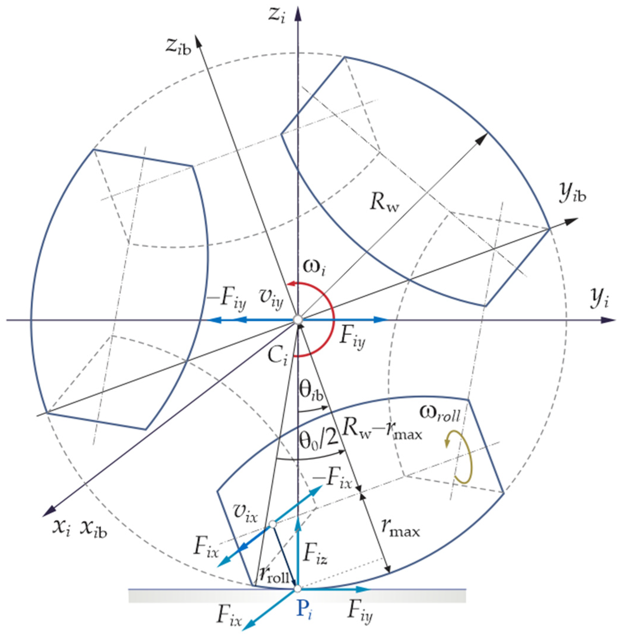
Figure 20 shows a side view of a wheel. Every wheel is driven by a DC motor over a geared belt and a planetary reducer. We describe the motion of the wheel with respect to the corresponding local coordinate frame C_ix_iy_iz_i. The angular velocity of the rotation of the wheel is ω_i, and it is directed along the x_i-axis (this is conventional—the real direction depends on the design of drivers’ chains and will be discussed later in relation to the wheels’ drivers).

In addition to rolling around the x_i-axis, the wheels may execute a side motion, i.e., in the direction of the x_i-axis, due to the rollers (Figure 20, see also Section 2.4). The roller that is in contact with the ground may freely rotate in its holder about its longitudinal axis, allowing for the side motion of the wheel. This motion is an essential characteristic of Robotino, because it allows it to move in any direction, irrespective of the current orientations of the wheels’ axes, i.e., they are omnidirectional. As already mentioned in the Introduction, omnidirectional wheels are of significant interest and are the subject of many studies [69,70,71,72].

Assuming that the rolling occurs without slipping, i.e., the velocity of the temporary contact point P_i is zero, the velocity of the wheel’s center is determined by:

$$v_i=v_{Pi}+v_{Ci/Pi}=\left(\begin{array}{c}0\\ 0\\ 0\end{array}\right)+\left(\begin{array}{c}{\omega }_i\\ 0\\ 0\end{array}\right)\times \left(\begin{array}{c}0\\ 0\\ R_w\end{array}\right)=\left(\begin{array}{c}0\\ -R_w\cdot {\omega }_i\\ 0\end{array}\right),$$

(8)

where R_w is the radius of the wheel.

Figure 20 shows the components of the reaction forces at P_i. Component F_iy is the reaction force opposing the slipping of the wheel on the ground during its rotation around the x_i-axis. Similarly, F_ix is the reaction of the ground to the slipping of the current roller during its rotation due to the sideways movement of the assembly along the x_i-axis. The component F_iz is the reaction that occurs due to the weight of the complete wheel assembly.

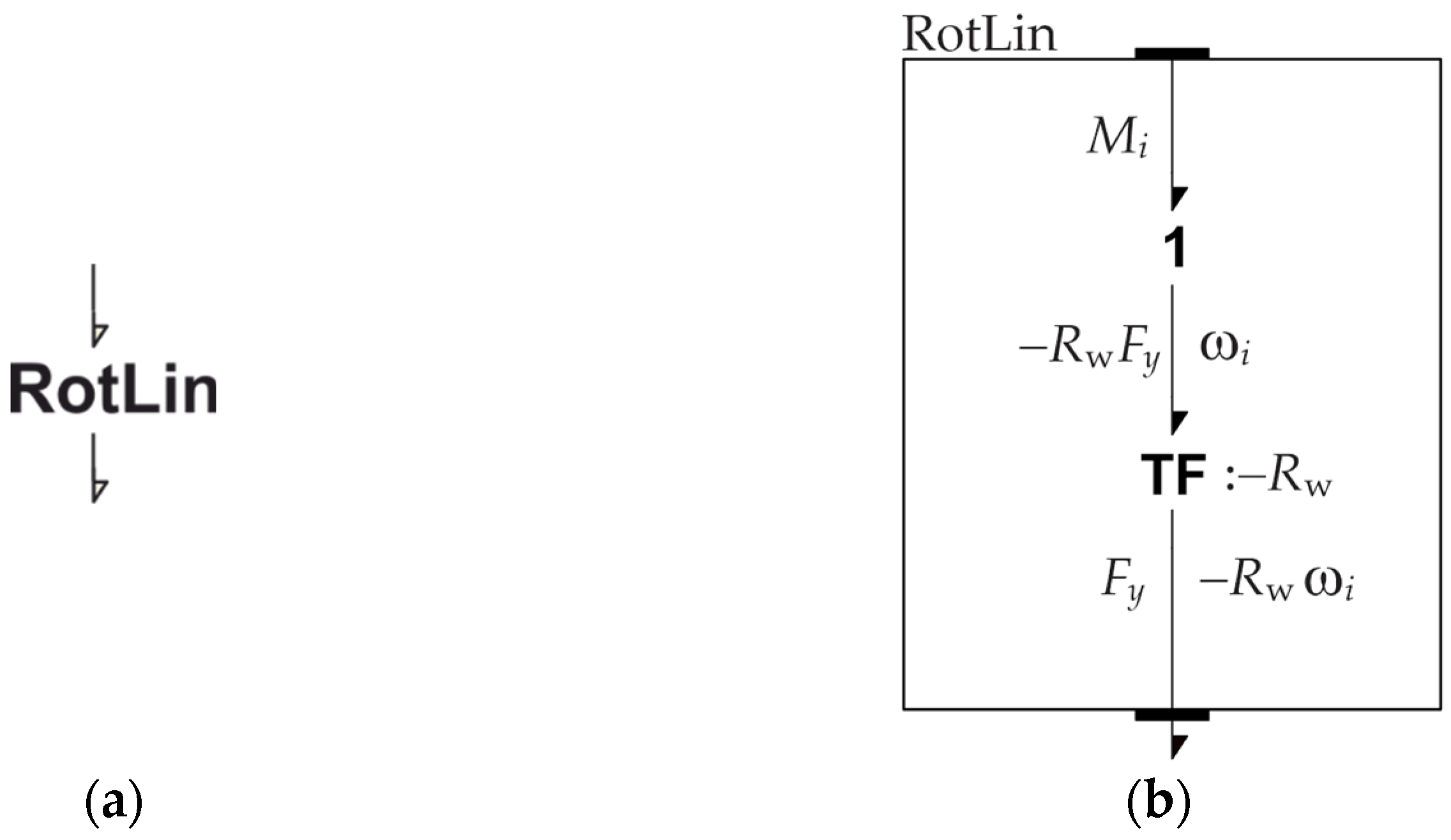
We reduce the F_iy component to the center C_i of the wheel (Figure 20). Hence, the respective moment with respect to point C_i is determined by:

$$M_i=\left(\begin{array}{c}0\\ 0\\ R_w\end{array}\right)\times \left(\begin{array}{c}0\\ F_y\\ 0\end{array}\right)=\left(\begin{array}{c}-R_w\cdot F_y\\ 0\\ 0\end{array}\right).$$

(9)

Hence, the rotation-to-linear-motion transform determined by (8) and (9) can be simply modeled by the RotLin component shown in Figure 21a, consisting of a single transformer TF in Figure 21b. It uses the parameter −R_w as the transformer arm.

We also introduce the wheel body-fixed frame x_iby_ibz_ib (i = 1, 2, 3), which overlaps with the x_iy_iz_i (i = 1, 2, 3) frame when the current roller touches the ground at its greatest diameter (Figure 20). Thus, the current body-fixed wheel frame is defined with respect to the current roller with which the wheel touches the ground. As the roller changes, the body-fixed frame changes as well.

We study the rotation of the wheel with respect to the world frame coordinates XYZ. However, we may also study it in the current wheel body-fixed frame. In this frame, the temporary contact point P_i apparently moves in the opposite direction.

When the wheel rotates around the x_i-axis by θ_i radian, the z_ib-axis rotates by an angle of θ_ib. We calculate a helper angle according to the expression:

$${\theta }_{temp}=\mathrm{mod}\left({\theta }_i,\pi /3\right).$$

(10)

Using a mod operator definition, this angle lies in the range [0, π/3]. However, as ${\theta }_0=\pi /3$, when this angle is greater than ${\theta }_0/2$, the contact point switches to the next roller, and the body-fixed frame changes accordingly (Figure 20). Therefore, to properly define angle ${\theta }_{ib}$ between the body-fixed z_ib-axis and z_i-axis, we set the following condition. Operators “?:” are known as the question operators and represent the inline version of if-then-else constructs:

$$\begin{array}{l}{\theta }_{ib}={\theta }_{temp}\ge 0 ? {\theta }_{temp}\le \pi /6 ? {\theta }_{temp}: {\theta }_{temp}-\pi /3\\ \hspace{1em}\hspace{1em}\hspace{1em}\hspace{1em}\hspace{1em} :{\theta }_{temp}\ge -\pi /6 ? {\theta }_{temp}:-{\theta }_{temp}-\pi /3\end{array}$$

(11)

Every roller can, by itself, freely rotate about its longitudinal axes (Figure 20). These axes form a plane, which is orthogonal to the wheel rotational axis. In this way, in addition to the normal rolling of the wheel around its rotational axis x_i, the wheel may move sidewise due to a roller currently in contact with the ground rolling about its longitudinal axis.

We can find the velocity arm r_roll (Figure 20) from the relationship:

$$R_w\cos \left({\theta }_{ib}\right)=r_{roll}+R_w-r_{\max },$$

(12)

or

$$r_{roll}=r_{\max }-R_w\left(1-\cos \left({\theta }_{ib}\right)\right).$$

(13)

Assuming that the rolling of the roller takes place without slipping, and applying the right-hand rule to the roller, we obtain:

$$v_{ix}=r_{roll}\cdot {\omega }_{iroll}.$$

(14)

Thus, the velocity of the wheel center is holonomic, i.e., it does not depend on the direction of the wheel axis.

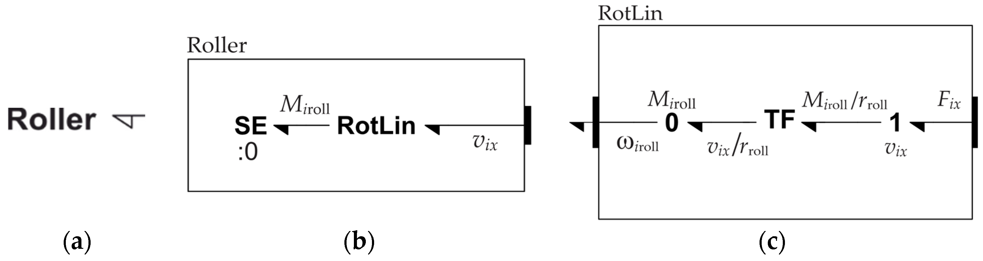
The model of the roller component is shown in Figure 22. Comparing this with Figure 21, it can be seen that the rotation is similar to that of the wheel, but with a different rolling arm.

Following these kinematical considerations, we turn to the dynamics of the wheel. Due its rotational symmetry, we assume that the wheel’s mass center coincides with its geometric center C_i. Thus, the motion of the wheel can be decomposed into its translation, which is determined by the motion of its center and its rotation around it. Because the wheels are joined to the Robotino’s base and translate with it, we may take into account the translational dynamics of the wheel when analyzing the motion of the chassis. Thus, all that remains is to analyze the rotational dynamics of the wheel.

We apply the moment of momentum law for rotation around the wheel’s center C_i. The moment of momentum with respect to the local frame x_iy_iz_i, (i = 1, 2, 3) reads as follows:

$$L_{Ci}=\left(\begin{array}{c}{I}_{ix}{\omega }_i\\ 0\\ 0\end{array}\right), (i=1,2,3),$$

(15)

where $I_{ix}$ is the moment of inertia of the wheel with respect to the x_i-axis. We transform (15) to the world frame XYZ by pre-multiplying by rotation matrix (3):

$$L_{Ci}^w=R_i\left(\begin{array}{c}{I}_{ix}{\omega }_i\\ 0\\ 0\end{array}\right)=\left(\begin{array}{c}{I}_{ix}{\omega }_i\cos \left({\phi }_i\right)\\ I_{ix}{\omega }_i\sin \left({\phi }_i\right)\\ 0\end{array}\right), (i=1,2,3).$$

(16)

Now, the moment of momentum law reads:

$${\displaystyle \frac{d{L}_{Ci}^w}{dt}}=M_i^w,$$

(17)

where $M_i^w$ is the applied moment. If we denote the net moment applied to the wheel by M_ix, we have:

$$M_i=\left(\begin{array}{c}{M}_{ix}\\ 0\\ 0\end{array}\right), (i=1,2,3).$$

(18)

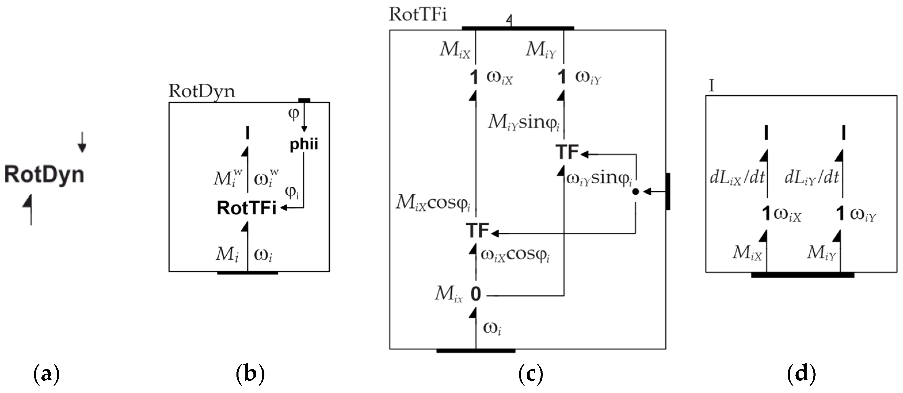
Using (16) and (18), we can write (17) as:

$${\displaystyle \frac{d}{dt}}\left(R_i\left(\begin{array}{c}{I}_{ix}{\omega }_i\\ 0\\ 0\end{array}\right)\right)=R_i\left(\begin{array}{c}{M}_{ix}\\ 0\\ 0\end{array}\right).$$

(19)

Figure 23 shows the bond graph component RotDyn describing (19). Note that the component RotTFi in the RotDyn document is the coordinate transform between the local x_i and world coordinates. Finally, the last component in Figure 23 represents the rotational dynamics of the wheel in the world frame.

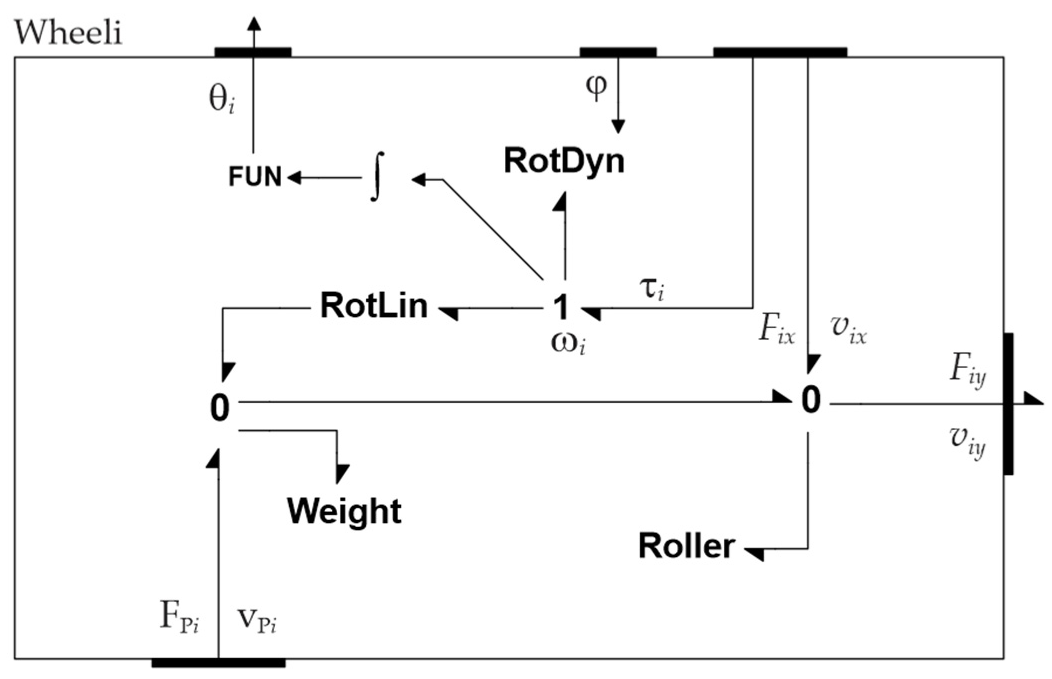
Finally, we formulate the bond graph model of the wheel, which contains all of the components that we discussed previously (Figure 24). The integrator serves to find the angle of the wheel rotation in radians, and the function converts the radians into degrees.

3.4. Dynamics of the Chassis

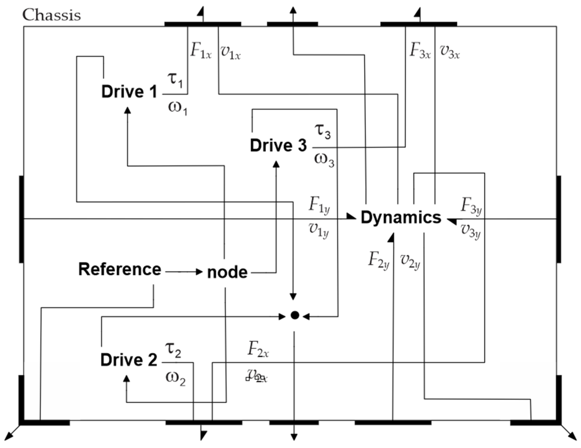
The bond graph model of the chassis is shown in Figure 25. The model follows the structure of the real device, which contains three drive units represented by the components Drive 1 to Drive 3. The drivers develop angular velocities ω_i and torques τ_i, which are applied to the wheels (Figure 24).

The component Dynamics in Figure 25 models the kinematics and dynamics of the chassis motion. We start from the relation between the velocity of the wheel centers in the local coordinates and the world velocity of the chassis center:

$$v_C^w={\left({\dot{X}}_C\hspace{1em}{\dot{Y}}_C\hspace{1em}0\right)}^T,$$

(20)

where X_C and Y_C are its coordinates in the world frame. This relation reads as:

$$v_i+v_{C/Ci}=v_C^i=R_i^T{v}_C^w,\hspace{0.33em}(i=1,2,3),$$

(21)

or

$$\left(\begin{array}{c}{v}_{ix}\\ v_{iy}\\ 0\end{array}\right)+\left(\begin{array}{c}0\\ 0\\ \dot{\phi }\end{array}\right)\times \left(\begin{array}{c}-R\\ 0\\ 0\end{array}\right)=\left(\begin{array}{ccc}\cos \left({\phi }_i\right)& \sin \left({\phi }_i\right)& 0\\ -\sin \left({\phi }_i\right)& \cos \left({\phi }_i\right)& 0\\ 0& 0& 1\end{array}\right)\left(\begin{array}{c}{\dot{X}}_C\\ {\dot{Y}}_C\\ 0\end{array}\right),\hspace{0.33em}\left(i=1,2,3\right),$$

(22)

where R is the radius of the circle, which contains the wheel centers (Figure 18). Expanding the last equation yields:

$$\begin{array}{l}{v}_{ix}={\dot{X}}_C\cos \left({\phi }_i\right)+{\dot{Y}}_C\sin \left({\phi }_i\right)\hspace{1em}\hspace{1em}\hspace{1em}\hspace{1em}\hspace{0.33em}\hspace{0.33em}(a)\\ v_{iy}-R\dot{\phi }=-{\dot{X}}_C\sin \left({\phi }_i\right)+{\dot{Y}}_C\cos \left({\phi }_i\right)\hspace{1em}\hspace{1em}(b), (i=1,2,3).\end{array}$$

(23)

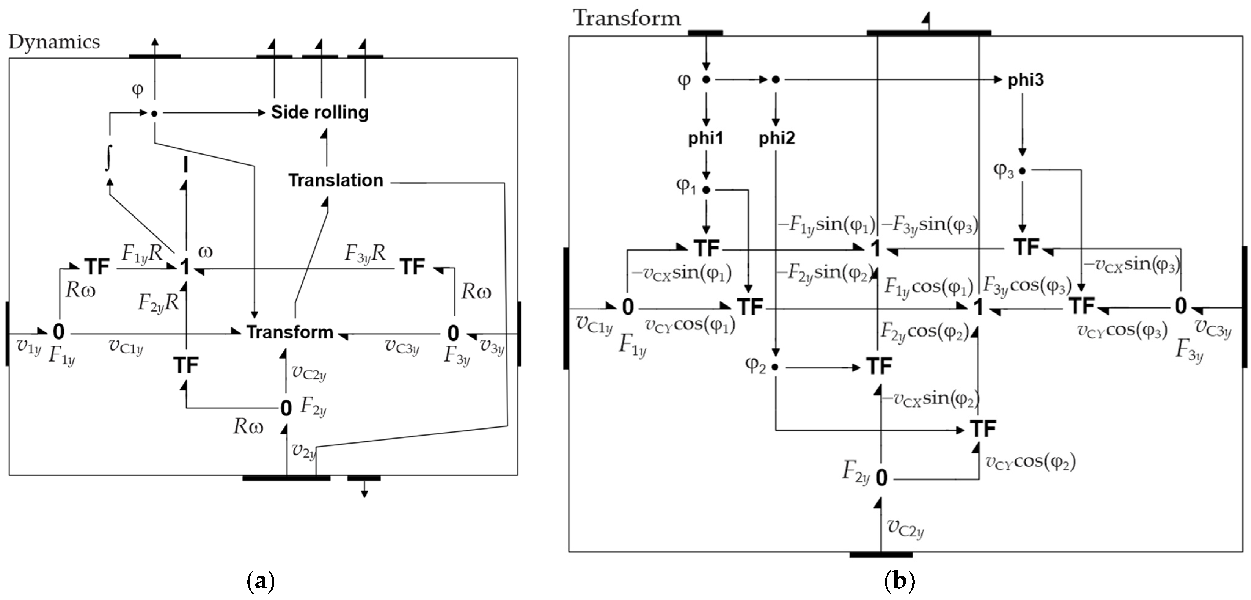
The bond graph model of the base dynamics is shown in Figure 26a. It plays a central role in Equation (23). The three transformers TF describe rotation-to-linear transformation (similar to Figure 21). They also generate the moments of the y-axis forces of the wheels acting on the chassis about their Z-axis. The Transform describes the right side of (23b) (Figure 26b). It also transforms the y-axis forces of the wheels acting on the chassis to the world frame and applies them to the center of mass of the assembly (see Translation in Figure 26a).

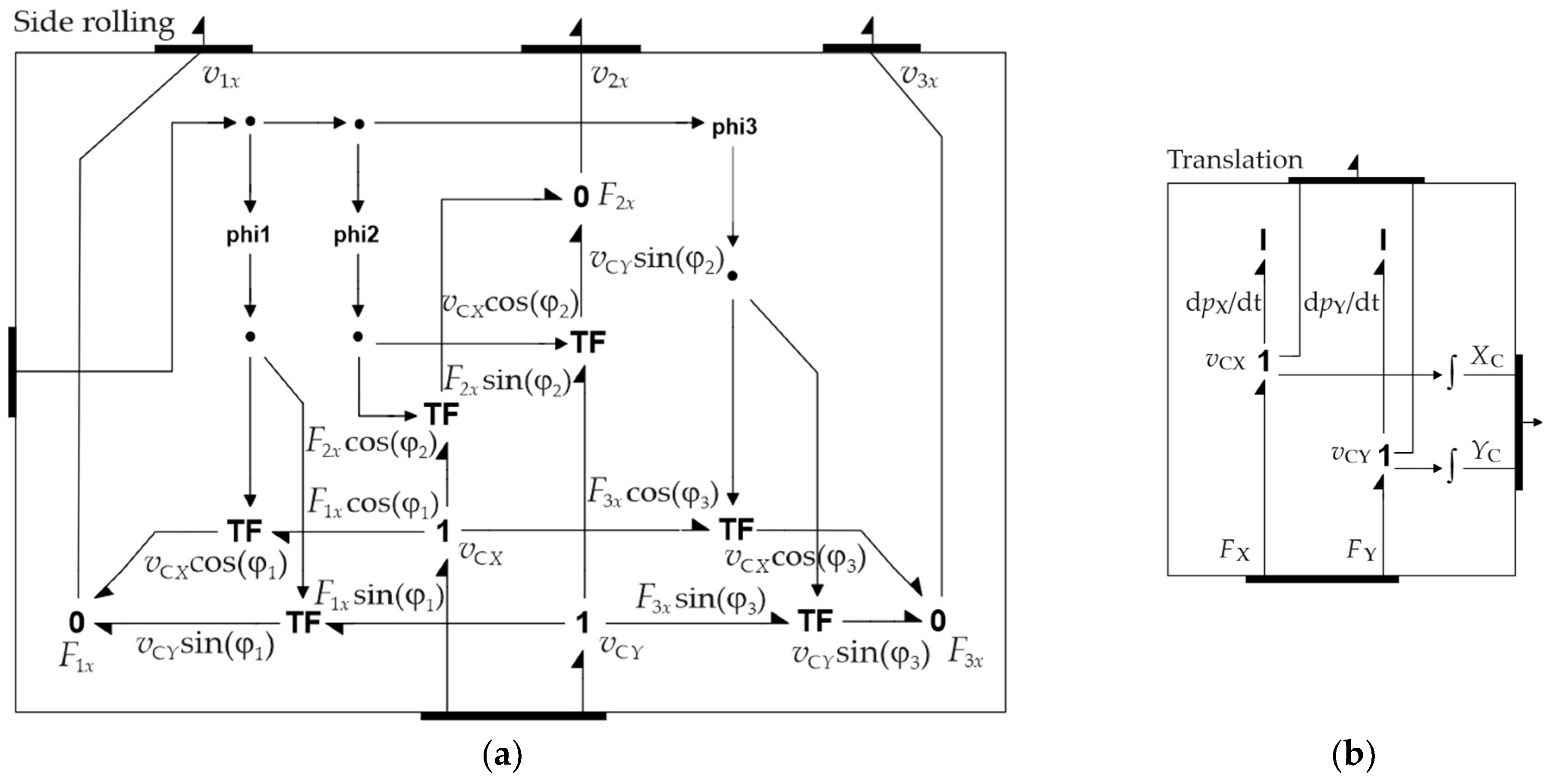
The Side rolling in Figure 26a describes the motion of the wheels due to the rotation of the rollers. The velocities of this motion are described by the bond graph representation in Figure 27a. It generates the x component of the wheel center, as defined by (23a). The roles of the transforms serve not only to transform the velocities of the chassis’ centers from world to local frames, but also to transform to the world frame the x-axis components of the forces acting as the rollers come into contact with the ground (Figure 20), which are transferred by the wheels to the chasses. The sum of these forces is transferred through the bottom port into Translation’s upper port (Figure 27b).

The component Translation describes the translational dynamics of the Chassis, including the wheels (Figure 27b). The inertial element I describes the translational dynamics of the chassis.

We now return to the model of Chassis in Figure 25. There are three Driver components, one for every wheel, which model the driver units of the Robotino.

Figure 28 shows the structure of the drivers. The drivers consist of DC motors [86] and reducers (belt drives and planetary reducers). The DC motors are modeled using gyrators (Damic and Montgomery [76]) and lossless reducers by simple transformers.

In this model, the control of the drivers is provided by common PID controllers. The reference angular velocity follows from (8) and (23b):

$${\omega }_i=-\left(R\dot{\phi }-{\dot{X}}_C\sin \left({\phi }_i\right)+{\dot{Y}}_C\cos \left({\phi }_i\right)\right)/R_w,\hspace{0.33em}(i=1,2,3).$$

(24)

The reference inputs are generated by the Reference component described in the next section. The positive direction of the motor rotation, following the right-hand rule, corresponds to the motor rotation axis directed into the Robotino’s body (see Figure 8). On the other hand, the wheels’ axes are parallel to these axes, but they are directed out of the body (See Figure 9). Therefore, the positive directions of angular velocities and torques on the sides of the motor and driver output are opposites.

This can be accounted for by setting the transformer ratio equal to the negative of the gear ratio, i.e.,

$${\omega }_i=-kgear\cdot {\omega }_m,{\tau }_m=-kgear\cdot {\tau }_i.$$

(25)

This also implies that the reference input in the feedback loop of Figure 28 should be scaled back by $-1/kgear$ before it is applied.

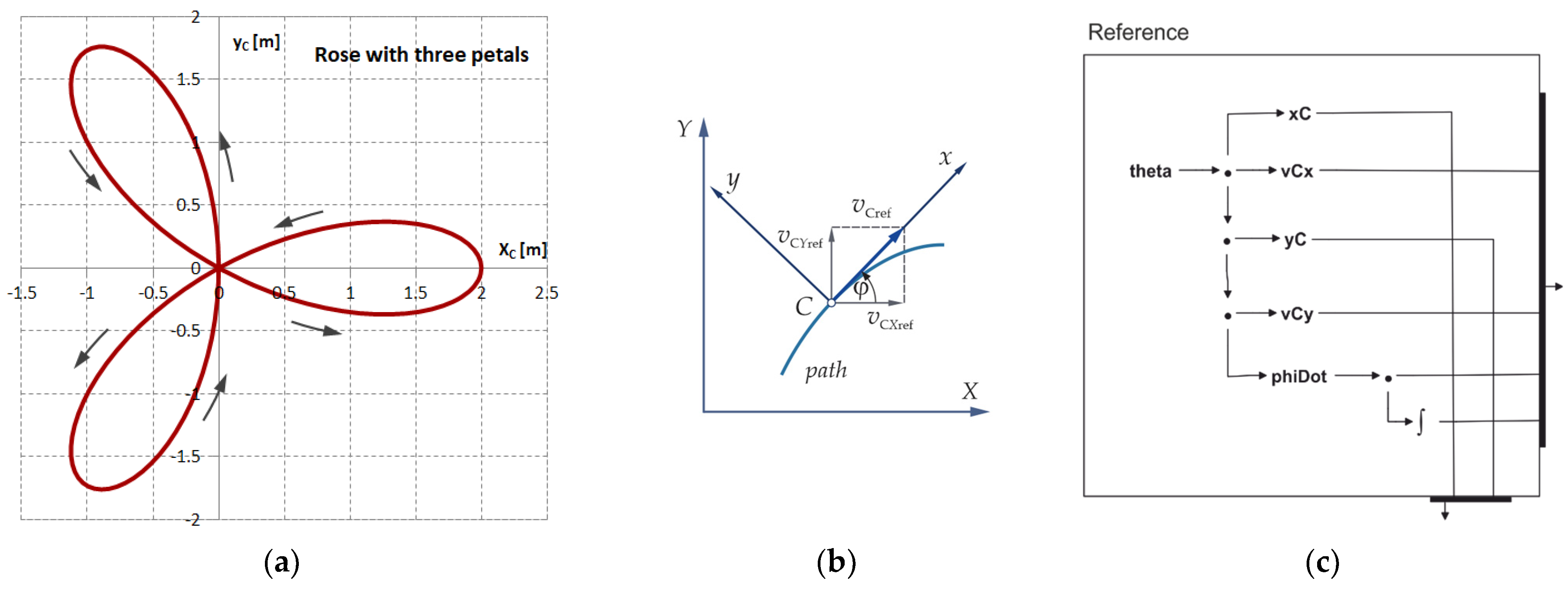
3.5. Planning of Motion

The purpose of the Reference component is to define the path of a plane curve that the center C of the Robotino’s bottom should follow, as well as the direction of its motion, and to generate the control signals for wheels driving. As an example of the curve, we use a (geometric) rose that is described by the following pair of Cartesian coordinates [87]:

$$\left.\begin{array}{l}{X}_{Cref}=ampl\cdot \cos \left(k\varphi \right)\cos \left(\varphi \right)\\ Y_{Cref}=ampl\cdot \cos \left(k\varphi \right)\sin \left(\varphi \right)\end{array}\right\}.$$

(26)

If parameter k = 3, then (26) describes a rose with three petals of amplitude ampl = 2 m (Figure 29a). We choose this relatively simple path because it will force Robotino to change the direction of its motion fairly often, and we can see whether the model we are developing simulates this motion correctly.

To describe the path shown in Figure 29a, we define parameter $\varphi$ as follows:

$$\varphi =a\cdot t+5\pi /6,$$

(27)

where a is a parameter, and t denotes the time. Note that, initially, X_C = 0, Y_C = 0, and the curve starts in the fourth quadrant with ampl of 2.0 m. To pass over all three petals, it needs π radians. Thus, if a = 0.1, it needs approximately 31.4 s for one complete cycle.

Differentiating (26) and (27) with respect to time, we find the expressions for the world velocity components of the Robotino center C along the reference path:

$$\left.\begin{array}{l}{v}_{CXref}={\displaystyle \frac{d{X}_{Cref}}{dt}}=ampl\cdot a\cdot \left(-k\sin \left(k\varphi \right)\cos \left(\varphi \right)-\cos \left(k\varphi \right)\sin \left(\varphi \right)\right)\\ v_{CYref}={\displaystyle \frac{d{Y}_{Cref}}{dt}}=ampl\cdot a\cdot \left(-k\sin \left(k\varphi \right)\sin \left(\varphi \right)+\cos \left(k\varphi \right)\cos \left(\varphi \right)\right)\end{array}\right\}.$$

(28)

The direction of motion is defined by assuming that the Chassis axis x is tangential to the reference path at the current position of the Chassis center C (Figure 29b). The corresponding angle φ is determined by:

$$\tan \left({\phi }_{ref}\right)={\displaystyle \frac{v_{CYref}}{v_{CXref}}}.$$

(29)

We find the reference angular velocity of the chassis by differentiating (29) with respect to time:

$${\omega }_{ref}={\cos }^2\left({\phi }_{ref}\right){\displaystyle \frac{d}{dt}}\left({\displaystyle \frac{v_{CYref}}{v_{CXref}}}\right)=a\cdot {\displaystyle \frac{2k^2{\sin }^2\left(k\varphi \right)+\left(k^2+1\right){\cos }^2\left(k\varphi \right)}{k^2{\sin }^2\left(k\varphi \right)+{\cos }^2\left(k\varphi \right)}}.$$

(30)

Now, to find angle φ_ref as a continuous function of ϕ, and thus of time t, we may integrate (30) using a suitable initial value, i.e.,

$${\phi }_{ref}={\displaystyle \underset{0}{\overset{t}{\int }}{\omega }_{ref}dt}.$$

(31)

We chose a rose with three petals as the reference path because it is relatively easy to generate using the equations above, and because it forces the center of the Robitino’s base to follow the curved path and continuously change its camera viewing direction to be tangential to the path.

The component Reference (Figure 29c) implements the above functional relationships consisting of the input function (27), the chassis center position (26), and the linear (28) and angular velocity functions (30), as well as the rotation angle (31). The outputs of these functions are forwarded to the drivers shown in Figure 25.

3.6. Basic Model of Robotino

Referring to the basic model of Robotino shown in Figure 17, we can conclude that we have developed bond graph models of all the system components—the chassis and three wheels. The model of the Ground still needs to be defined.

The main role of the ground is to hold the Robotino and apply friction to its wheels. We simplify the effect of friction by assuming that the Robotino’s wheels do not slide over the ground. Thus, the model of Ground is very simple (see Figure 30). The action of the floor is modeled by the three components vP1 to vP3, acting at the current contact points P1–P3 (Figure 30a). They each contain three source flows (SFs) (Figure 30b), which impose the zero-velocity components of the current wheel’s connection point in the direction of world axes. The corresponding reaction forces depend on the dynamics of the Robotino’s motion.

Finally, we complete the model shown in Figure 17 by adding the missing components—i.e., the displays and the named pipe interface IPC. These components require corresponding signals; thus, we also add the components consisting of signal nodes to help in distributing the signals over the system. The resulting model is shown in Figure 31.

3.7. Building the Mathematical Model and Solving It Using the Backward Differentiation Formula (BDF)

Before we start the simulation, we need to build the mathematical model of the hierarchical bond graph model. Starting from this root (i.e., basic) level model, we pass the model tree several times. First, we check that every component is correctly connected, and next we generate the system variables in terms of how we define its mathematical model. After that, we assess all the elementary components, reading their constitutive relations. We translate their form as described in Table 1 into the implicit forms. Thus, e.g., the constitutive relations of the left flow junction of Figure 26b are connected to the transformers, as described by the following equations:

$$\begin{array}{l}{v}_{C1y}+f_1-f_2=0,\\ f_1+v_{CX}\sin \left({\phi }_1\right)=0,\\ f_2-v_{CY}\cos \left({\phi }_1\right)=0.\end{array}$$

(32)

Similarly, the constitutive relations of the inertial elements in Figure 27b are expressed as:

$$\begin{array}{l}{\displaystyle \frac{d{p}_X}{dt}}-F_X=0,\\ {\displaystyle \frac{d{p}_Y}{dt}}-F_Y=0.\end{array}$$

(33)

Next, we translate them into the prefix form. Thus, the common infix form a + b = c is translated into the prefix form +ab, and a similar process is carried out for other expressions. In these forms, the left side of a relation can be more efficiently evaluated and translated in Microsoft’s net assembly (using the cli extension of the C++ language). We collect the processed constitutive relations in a list of relations.

After all the model equations are collected, we visit them again and generate the expressions for the elements of the corresponding partial derivative matrix. We evaluate this via symbolic partial derivation. In this way, both the equations and the element of partial derivative matrix are expressed symbolically in order to improve the solution of the DAE equation.

We can represent the mathematical model generated in the matrix form as:

$$\left.\begin{array}{l}\dot{x}-z=0,\\ f\left(x,y,t\right)=0\end{array}\right\}.$$

(34)

The first equation corresponds to the inertial, capacitive, and integrator comports, and the second to the rest of the component constitutive relations. Taking the time derivation of Equation (34), we obtain:

$${\displaystyle \frac{\partial f}{\partial x}}\dot{x}+{\displaystyle \frac{\partial f}{\partial y}}\dot{y}+{\displaystyle \frac{\partial f}{\partial t}}=0.$$

(35)

Taking into account Equation (34), we can write the last equation in the form:

$${\displaystyle \frac{\partial f}{\partial y}}\dot{y}=-\left({\displaystyle \frac{\partial f}{\partial x}}z+{\displaystyle \frac{\partial f}{\partial t}}\right).$$

(36)

Thus, if the Jacobian matrix ${\displaystyle \frac{\partial f}{\partial y}}$ is invertible, we can express the time-derivate of $y$ as:

$$\dot{y}=-{\left({\displaystyle \frac{\partial f}{\partial y}}\right)}^{-1}\left({\displaystyle \frac{\partial f}{\partial x}}z+{\displaystyle \frac{\partial f}{\partial t}}\right).$$

(37)

Therefore, the second part of Equation (34) has a differentiation index 1; taken together with the first, we deduce that (34) has an index 2 DAE (see Brenan et al. [88], p. 39).

Well-known Backward Differentiation Formulas (BDFs) have emerged as one of the best methods for solving general DASs. Brenan et al. [88], pp. 54–56, showed that, when applied to a model (34), the k-step BDF (k < 7) is convergent to the order of h^k, where h is the current step size. BondSim uses only one integrator, the general form of the Backward Differentiation Formula (BDF), i.e., its variable coefficient form method [76], to solve bond graph models. In comparison, the famous DASSL uses the constant coefficient form of BDF [88]. It is well known that the variable coefficient form of BDF is the most stable version of BDF, but it requires more frequent evaluation of the partial differentiation matrix of the DAE system (the Jacobian system). This is counterbalanced in BondSim by generating this matrix in a sparse analytic form, as described above. In addition, the equations of the mathematical model of the problem and the corresponding expressions of the matrix elements are internally converted into the NET assembler form using Microsoft’s C++/CLR language extension. They can therefore be evaluated efficiently (in DASSL, this matrix is evaluated numerically). For details, see Damic and Montgomery [76].

Hence, we may conclude that the equations of a mathematical model can be successfully solved using the BDF method if they are independent. This is relatively easy to achieve by applying the bond graph method, as described in [76], and by following the structure of the physical system under consideration.

To start the simulation process, after the mathematical model has successfully been built, we apply the menu command Run. A dialog window opens, which is used to input the simulation parameters (simulation time, output interval, maximum step size, absolute and relative errors, etc.). After the OK button is pressed, the simulation starts.

3.8. Named Pipe Communications and Simulation

The named pipe is a two-way IPC mechanism, which enables the transfer of data between two or more applications on the same computer, or on computers connected in a local net. Any applications can serve both as server and a client, making two-way communications possible. However, only one application creates the named pipe: it is termed the server. Those that connect to the first application are called clients.

In this scenario, there is one server, BondSim3DVisual, and one client, BondSim implemented on the same computer. After a project is opened on the first one and the scene is created, we create the named pipe using the command Open Pipe. After the pipe is created, a message is sent inviting the client to connect to it.

To connect to the server, we activate the BondSim applications and open the bond graph problem corresponding to the virtual project we created in the server. We manipulate the frames of both applications to make them both visible on the computer screen.

The bond graph model contains an IPC component in the form of a ring (or pipe cross-section) (see the top of Figure 31). It has an input signal port that serves to connect the signal lines, which transfer data across the pipe to the server, and an output port that receives the signal data returned by the pipe. After all the IPC ports are connected, we build a mathematical model of the BondSim application. If the building of the model is successful, we can start the simulation. Before starting the simulation, we need to connect it to the server using the corresponding command under the Build menu.

There is one other parameter that needs to be defined at the start of simulation. This is the Frames per second (FPS) parameter. The visual screen in BondSim3DVisual is updated by sending data over the pipe at discrete times. Every pack of data generates a picture displayed on the screen; this is called a frame (following film terminology). The question of how often we need to send data is answered by the fact that the human brain can process 10 to 12 FPS, which are received by our eyes as steady pictures; higher rates are recognized as motion. The time interval when the packs are sent over the tube is currently set to 30 ms, or about 33 FPS.

Every pack of data that is sent by the client consists of a series of binary values of the joint drive’s angular or prismatic displacement (see Figure 6b), ordered by counting joints in the XML model tree starting from the root and moving to the tree top (Figure 10). Thus, the first value corresponds to the first joint bellow the root, the second datapoint to the next joint, etc. After the pack is received by the server, it reads it and sends the first datapoint to the first joint drive, the second to the second joint drive, etc. Thus, the pack coding is very simple and easy to decode. After receiving data, the geometry of the mechanism is reevaluated and the screen updated. Repeating the package sending and updating the screen appears as the motion of mechanism over the screen.

A similar observation can be made of the date packs sent from the server to the client. Because these data currently contain only the coordinates of the probe (in the Robotino model, a small red ball below its body), when received by the client, these have to be taken into account.

4. Simulation of Robotino’s Path

We can now simulate the motion of Robotino along the planned path. We build the model first and then start a simulation run using the following parameters: simulation interval 50 s, output interval 0.02 s, maximum time step size 0.02 s, errors 1 × 10⁻⁶. The simulations are performed on a PC with a x64-based processor, AMD Ryzen 7 PRO 4750 G (AMD, Santa Clara, CA, USA), with Radeon Graphics 3.60 GHz. The total elapsed time is 0.51 s. After that, we repeat the simulation with the same parameters, and this time, we enable communication between the dynamic and virtual models. Communication is established using the IPC pipe component (inter-process communication), shown as a red ring in Figure 31, which enables the dynamic model to send some information. In our case, these are joint angle values, which are sent to the virtual model 30 times per second. When the dynamic model is connected to the virtual one, the total elapsed time is 46.83 s. Having tested the behavior of Robotino using both these models, in future investigations, we plan to connect them with a real physical robot according to the digital twin concept.

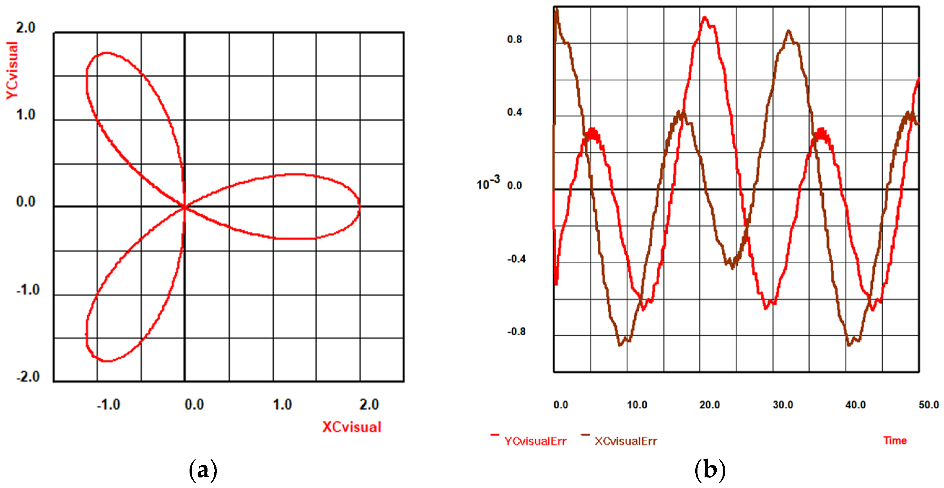
The BondSim3DVisual application also enables the mechanism movements to be written over the screen on a video file in the MP4 format. We start writing using the command Start Video and end it with the command End Video under the File menu. We can read this file using various applications, such as Media Player, Movies & TV, and similar. We uploaded this file to YouTube under the name Project Robotino, where readers can view it. When the video writing is underway, the process is somewhat slower, but it remains at about 50 s.

Some generated plots are shown in the figures below. The path coordinates in the plane motion sent to the virtual model force the latter to change its position on the screen, i.e., it moves. The corresponding virtual path coordinates are picked up by the probe element (Figure 10a) and sent back over the named pipe; they appear at the output of the IPC element. Figure 32a shows the corresponding path, as seen on the display connected to this IPC port. The difference between these signals and the signals of the Robotino’s base coordinates, which are evaluated using the simulation, i.e., the same signals that we previously sent over the pipe, are evaluated by the block below and to the right of IPC’s output port. They are displayed on the display component on the right. The resulting plot is shown in Figure 32b.

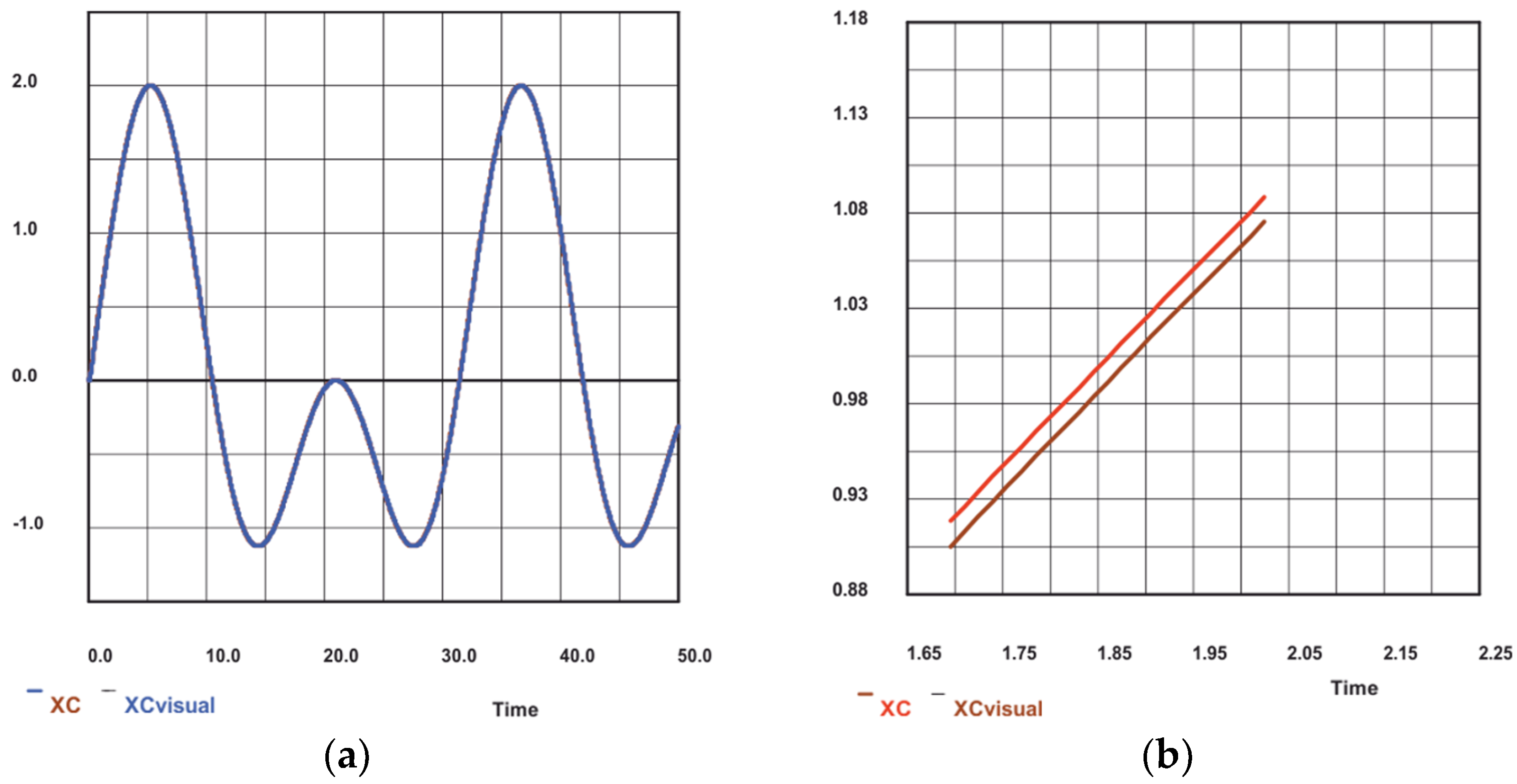
To further explain the obtained results, we put the x-coordinates of the center point XC and XCvisual on the same y-axis on the display at the right of the IPC component. This is shown in Figure 33a. At first glance, they appear to be a single curve. We expand a small rectangle around a point on the curve. The generated enlarged plot is shown in Figure 33b. There are really two curves, displaced by 30 ms (milliseconds). Thus, the signal sent back over the pipe is delayed by this time value; as a result, the accuracy of this curve is moderate, as shown in Figure 32b. The accuracy depends on the frequency with which data packs are sent over the pipe. In this simulation, it is exactly the same number, i.e., 30 ms.

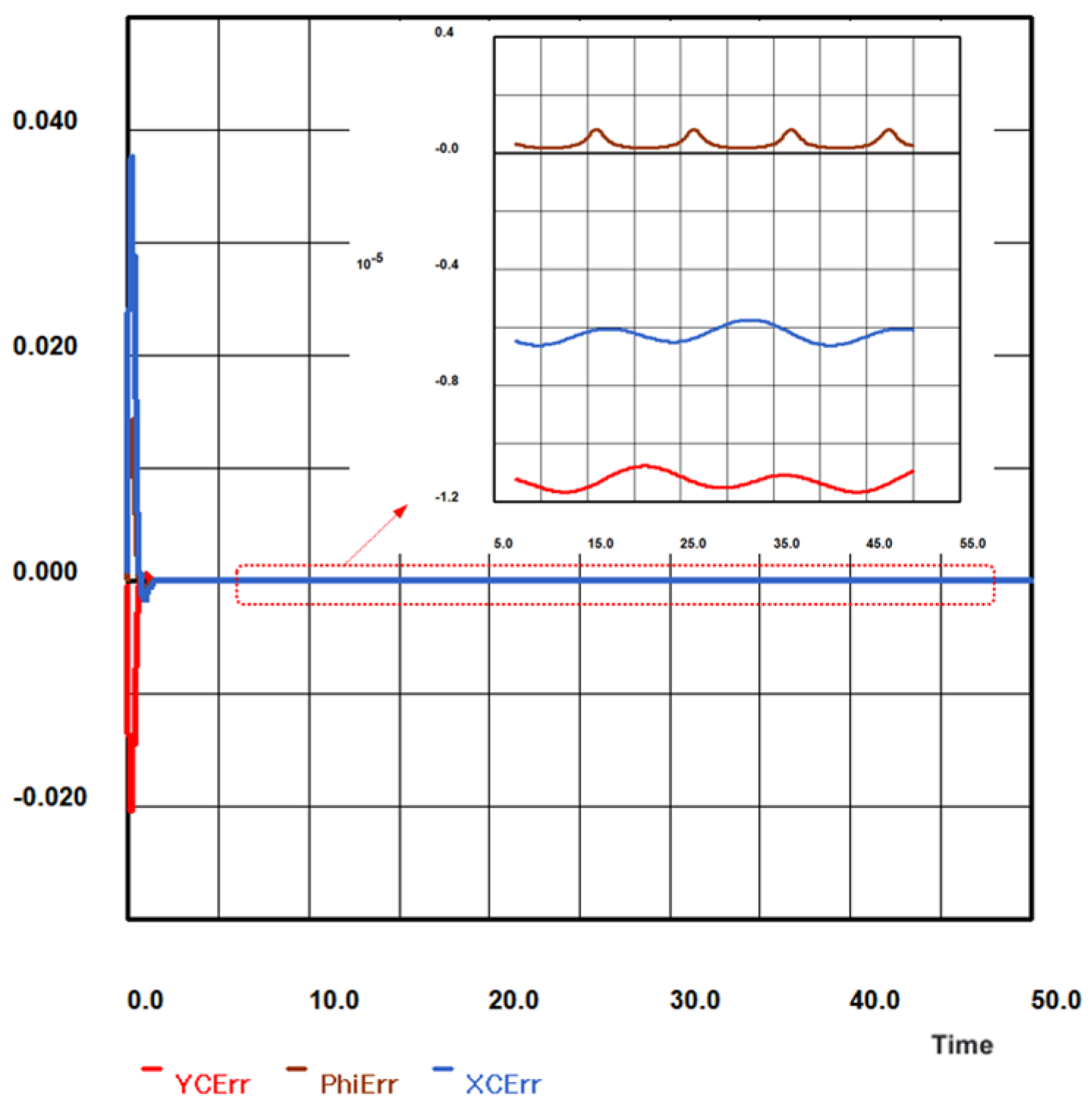
To verify the developed dynamic model and control algorithm, we compared the coordinates of the robot center and its orientation as obtained during the simulation with the reference values. Figure 34 depicts the deviations in the obtained coordinates of the Robotino’s center (X_C and Y_C) and its orientation (angle φ in radians) with reference to the reference values defined by (24) and (29). They are of the order of several 10⁻⁶ m for Xc, less than 2·10⁻⁵ m for Yc, and 10⁻⁶ rad for the angle φ (after the initial transient processes). This represents very good agreement. Note that the amplitude of the path is 2.0 m.

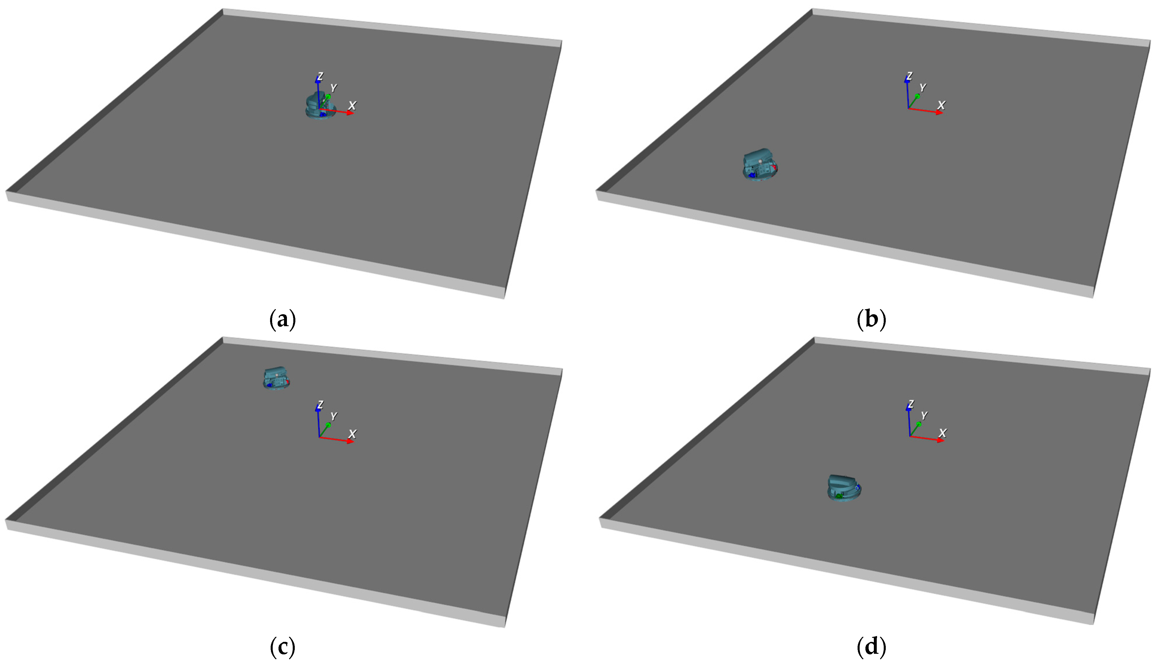
A virtual model of Robotino, captured at different time points during the simulation, is shown in Figure 35.

5. Conclusions

This paper proposes a novel methodology for the virtual 3D modeling of the articulated mechanisms that can be driven by signals obtained from other models: for instance, from its dynamic model developed using other software packages.

The proposed approach uses well-known XML technology, which provides the systematic development of a 3D visual model in the form of a tree. Instead of editing the XML document, the operations are applied to the document tree in the Tree View pane by inserting or removing the elements or attributes in the BondSim3DVisual environment. At the same time as generating a DOM-like tree, conventional XML code is also automatically generated and written into a separate read-only document window (with an XmlOutput pad).

The methodology explained here is applied to the modeling of a holonomic mobile robot (Robotino) equipped with three omnidirectional wheels. A 3D model of Robotino is created using 3D CAD models of robot parts in the form of STL files. The virtual driving of the articulated model by external signals is enabled by developing a dynamic model of the robot using the separate general-purpose bond graph software BondSim. During the development of the dynamic model of the robot, the lateral rolling of the robot’s omnidirectional wheels was also taken into account.

We established two-way communication between the two developed robot models—the dynamic and the virtual. During the simulation, both models run in different software packages and can communicate with each other. The dynamic model sends information to the virtual one to drive it, but there is also communication in the opposite direction. This means that some information can be picked up from the virtual model and delivered to the dynamic one (or to any other model). Thus, some information that can be more easily obtained using the virtual model can be delivered from the virtual side to the dynamic side. To verify the methodology presented here, a geometric rose with three petals was used as an example of the plane curve that the center of the Robotino should follow.

In future research, we aim to develop a more complex visual model of the environment in which the robot moves. This will enable us to establish communication between the dynamic model; the virtual model; and the real, physical robot—i.e., the Robotino, which is equipped with a complex sensor system to optimize its motion.