Identification of Natural Sloshing Frequency in a Rectangular Tank Under Surge Excitation Using Coupled Eulerian–Lagrangian Method and Impulse Excitation Method

Abstract

Sloshing in liquid storage tanks is a critical phenomenon that affects the stability, performance, and safety of various engineering systems, including fuel tanks, offshore structures, and industrial storage units. The presence of internal structures, such as vertical baffles, significantly influences the natural sloshing frequencies and fluid motion. However, existing theoretical models often rely on simplified assumptions that restrict their capacity to capture the complexities of fluid–structure interactions in baffled tanks. This study integrates the coupled Eulerian–Lagrangian method with the impulse excitation technique to predict natural sloshing frequencies in a rectangular tank with vertical baffles. By analyzing the system’s response to an impulse excitation, we extracted the dominant sloshing frequencies while considering the impact of baffles on fluid dynamics. This computational approach provides a more realistic representation of sloshing phenomena and enables a parametric analysis of how various tank dimensions, fluid properties, and baffle configurations influence sloshing behavior. The findings of this study contribute to the improved design and optimization of liquid storage tanks, ensuring enhanced stability and performance in practical engineering applications. The integration of impulse excitation with the coupled Eulerian–Lagrangian method marks a significant advancement in sloshing analysis, offering a robust framework for understanding and mitigating the effects of sloshing in baffled tanks.

1. Introduction

Sloshing, the fluid motion within containers, is a critical phenomenon in various engineering applications, including liquid storage tanks, fuel tanks in vehicles, and offshore structures. The natural sloshing frequencies of liquids significantly influence the dynamic response of these systems, affecting their stability, performance, and safety. Accurate prediction of sloshing behavior, especially considering various tank configurations, is essential to ensure optimal design and prevent undesired resonances or vibrations [1,2,3,4,5,6].

Traditional methods for estimating the natural sloshing frequencies of a liquid in a tank typically rely on simplified assumptions, such as a rigid tank, uniform fluid depth, and the absence of internal obstructions. One of the most widely used models, the shallow water theory, approximates sloshing behavior based on tank geometry and fluid depth [7,8,9]. However, these models have limitations in capturing the complexities of real-world systems, especially those with internal structures such as vertical baffles, which significantly affect sloshing frequencies and fluid motion.

Among various internal structures affecting sloshing dynamics, vertical baffles are particularly influential due to their damping and flow-altering effects. They are commonly installed in industrial tanks to mitigate excessive sloshing, enhance liquid mixing, and prevent the formation of high-amplitude waves. Baffles influence the fluid’s dynamic response by modifying flow patterns and increasing damping effects. Various studies have investigated the role of vertical baffles in sloshing mitigation. Akyildiz and Ünal (2006) examined sloshing loads in a moving, partially filled rectangular tank using both numerical and experimental approaches, employing the volume-of-fluid (VOF) method and validating the results against experimental data [10]. Liu and Lin (2009) explored sloshing suppression by vertical baffles using a virtual boundary force method and highlighted their effectiveness in reducing fluid motion [11]. Ma et al. (2021) studied the impact of single and double vertical baffles on violent sloshing, emphasizing the importance of baffle arrangement in enhancing damping by measuring liquid elevation, energy dissipation, and impact pressures [12]. Jung et al. (2012) analyzed the effect of baffle height on liquid sloshing in a laterally oscillating, three-dimensional rectangular tank, showing that higher baffles weaken vortex structures at their tips and thus influence the damping effect [13].

In addition to the structural effects of baffles, recent studies have emphasized that bubble or cavity formation during sloshing can significantly influence nonlinear fluid behavior. The formation of bubbles introduces complex fluid–structure interactions that alter the dynamic response beyond the predictions of linear theory. Chen et al. (2024) demonstrated through numerical simulations that gas inflow into dual liquid tanks intensifies sloshing behavior and increases impact forces on tank walls [14]. Yang et al. (2023) validated computational models capable of capturing detailed sloshing dynamics, including bubble formation and violent surface breakup, and showed good agreement with experimental observations [15].

Despite the practical significance of baffles, the impact of internal structures on natural sloshing frequencies remains insufficiently understood, and only a limited number of theoretical models predict these effects. Shin et al. (2006) analyzed the natural frequencies of sloshing in prismatic tanks with bottom baffles, employing a variational method and introducing the concept of effective liquid fill-depth to modify traditional frequency estimations [16]. Hu et al. (2018) extended this analysis by using a boundary element method (BEM) to study natural frequencies and mode shapes in two-dimensional baffled tanks, proposing empirical formulas for sloshing frequency prediction [17]. However, these analytical approaches generally assume linear fluid motion and two-dimensional simplifications, limiting their ability to capture three-dimensional and nonlinear behaviors in baffled tanks.

To address these limitations, advanced computational techniques have been increasingly adopted. In particular, the coupled Eulerian–Lagrangian (CEL) method has emerged as a powerful tool for modeling fluid–structure interactions (FSIs) and capturing the complex dynamics of sloshing phenomena [18]. The CEL method treats the fluid domain using a fixed Eulerian mesh while modeling solid structures, such as tank walls and baffles, with a moving Lagrangian mesh. This dual approach enables accurate simulation of large free surface deformations, flow separation, and vortex generation around internal structures, making it particularly suitable for analyzing sloshing in baffled tanks.

To further enhance the accuracy of natural frequency prediction, this study integrates the impulse excitation technique (IET), a well-established experimental method, into the numerical framework. The IET involves applying a brief, high-intensity impulse to the system and analyzing the resulting dynamic response to extract natural frequencies. It is particularly effective for identifying resonance peaks within the frequency spectrum, offering a clear and robust means of characterizing dynamic behavior [19,20].

In this study, we integrated the IET into a CEL-based finite element model to achieve accurate predictions of natural sloshing frequencies in a rectangular tank equipped with vertical baffles. By simulating the tank’s response to impulse excitation, we extracted the natural frequencies while explicitly accounting for the dynamic modifications introduced by baffles. This computational approach not only improves the realism of sloshing modeling but also enables systematic parametric studies to investigate the influence of various tank dimensions, fluid properties, and internal configurations on sloshing frequencies.

While existing analytical models rely on simplifying assumptions that often neglect detailed fluid–structure interactions, the present approach provides a more comprehensive and accurate analysis of sloshing dynamics. The integration of impulse excitation with the CEL technique represents a significant advancement in the numerical modeling of sloshing phenomena, offering a robust framework for understanding the influence of baffles on natural sloshing behavior.

This study focused on the lowest natural sloshing frequency because it typically governs the dominant dynamic response of liquid-filled tanks and is most critical for ensuring structural stability and avoiding resonance in practical engineering applications. This focus aligns with established practices in sloshing research, where the first mode often contributes the largest amplitude and energy. Nonetheless, it is acknowledged that higher-order modes can become important in certain scenarios, such as in large tanks, tanks with complex internal structures, or under high-frequency external excitations. A comprehensive analysis including higher modes remains an important direction for future research.

2. Theoretical Background

2.1. Closed-Form Solutions to Sloshing Natural Period of a Tank with Vertical Baffles

When a rectangular tank undergoes translational motion as described by Equation (1), the natural sloshing period of the liquid inside the tank, derived from linear theory, can be expressed as Equation (2). Here, $A$ is the amplitude, and $\omega$ is the angular frequency. $g$ is the acceleration due to gravity, $k$ is the wave number, where $k=m/L$, with $m$ representing the mode number. $L$ is the length of the tank, and $h_w$ is the water depth. Due to the nonlinear nature of the sloshing phenomenon, exact resonance may not always occur even when predicted by Equation (2). However, experimental studies have confirmed that for the lowest mode, the calculated values closely matched the observed results [10].

$$x=A\sin \left(\omega t\right)$$

(1)

$$T=\sqrt{{\displaystyle \frac{4{\pi }^2}{gk\tanh \left(k{h}_w\right)}}}$$

(2)

When a baffle is installed to suppress fluid motion inside the tank, the liquid flow characteristics within the tank change. Specifically, the presence of the baffle at the bottom of the tank results in an effect similar to a reduction in the water depth. Shin et al. (2006) applied linear theory based on potential theory and introduced the concept of effective fill-depth to express the sloshing natural period, as shown in Equation (3) [16]. Instead of the water depth, the effective fill-depth, which accounts for the baffle’s influence, is defined as $h_e=h_w-\beta h_b$. Here, $\beta$ is the depth reduction coefficient for a configuration where baffles of height $h_b$ are arranged at equal intervals with $n_b$ baffles on the tank floor.

$$\begin{gathered} T=\sqrt{{\displaystyle \frac{4{\pi }^2}{gk\tanh \left(k{h}_e\right)}}} \\ \mathrm{where} \beta =1-{\gamma }^2{\displaystyle \frac{n_b+1}{2}}{\displaystyle \frac{\tanh (n_b+1)k{h}_b}{\tanh \left(k{h}_b\right)}}, \gamma ={\displaystyle \frac{4}{\pi }}{\displaystyle \frac{n_b+1}{{n_b}^2+2n_b}}cos\left\{{\displaystyle \frac{\pi }{2(n_b+1)}}\right\} \end{gathered}$$

(3)

Hu et al. (2018) also developed a closed-form equation to calculate the natural sloshing period of a tank with vertical baffles based on potential theory [17]. Unlike Shin et al. (2006) [16], they identified the ratio of water depth to tank length as a key parameter. Based on this parameter, they organized the analysis results, obtained using the boundary element method, for tanks with various geometries and developed fitting equations for these results. They proposed an empirical formula, as shown in Equation (4), based on these fitted results.

$$\begin{gathered} T=\sqrt{{\displaystyle \frac{h_w}{g\pi {\left(\frac{h_w}{L}\right)}_{eff}\tanh \left[{\pi \left(\frac{h_w}{L}\right)}_{eff}\right]}}} \\ \mathrm{where} {\left({\displaystyle \frac{h_w}{L}}\right)}_{eff}={\displaystyle \frac{h_w}{L}}·\left[1-e^{-E\left(n,{\displaystyle \frac{h_w}{L}}\right){\left(1-{\displaystyle \frac{h_b}{h_w}}\right)}^{F\left(n,{\displaystyle \frac{h_w}{L}}\right)}}+e^{-E\left(n,{\displaystyle \frac{h_w}{L}}\right)}\right] \\ E\left(x,y\right)=0.4138-0.4973x+3.386y+0.03317x^2+0.5107xy+0.1182y^2, \\ F\left(x,y\right)=0.1848+0.1329x+0.4365y-0.01212x^2+0.0002057xy-0.1094y^2 \end{gathered}$$

(4)

2.2. Impulse Excitation Technique

The Impulse Excitation Technique (IET) is a widely used experimental method for determining the natural frequencies of dynamic systems. This technique involves applying a short, high-energy impact to the system and measuring its subsequent response. By analyzing this response, the natural frequencies of the system can be accurately identified [19,21].

The core concept of the IET is to apply a short-duration force or impulse to a system, exciting its natural vibration modes. The system’s response to this excitation is recorded, typically using sensors such as accelerometers or displacement transducers. The resulting time-domain signal is then analyzed to determine the system’s natural frequencies. Mathematically, the response of a simple linear system to an impulse excitation can be described by the following equation:

$$x\left(t\right)=A \sin ({\omega }_{n}t+\varphi )e^{-\zeta {\omega }_{n}t}$$

(5)

where $x\left(t\right)$ is the system’s response over time. $A$ is the amplitude of the response, and ${\omega }_n$ is the natural frequency of the system (rad/s). $\zeta$ is the damping ratio (dimensionless), $t$ is time, and $\varphi$ is the initial phase.

For lightly damped systems, the response typically oscillates at a characteristic frequency, which is primarily governed by the system’s natural frequency. By measuring the response and fitting it to the corresponding equation, the natural frequency of the system can be determined. In practice, the time-domain response is transformed into the frequency domain using the Fourier Transform method, allowing for a more precise identification of the dominant frequencies.

$$X\left(\omega \right)={\int }_0^{\infty }x(t)e^{-i\omega t}dt$$

(6)

where $X\left(\omega \right)$ is the frequency response function, and $\omega$ is the angular frequency.

From the frequency-domain representation, the natural frequency can be identified as the peak in the spectrum. The main peak corresponds to the system’s fundamental natural frequency. For damped systems, the amplitude of the peak will be smaller, but the natural frequency can still be determined accurately from the spectral content.

2.3. Coupled Eulerian–Lagrangian Method

In simulations involving fluid–structure interactions, such as sloshing in a liquid tank, it is essential to account for significant fluid deformation and the interface between the fluid and the solid structure. Directly applying the traditional Lagrangian formulation to model the fluid domain can be impractical due to excessive distortion of fluid elements, particularly under high-deformation conditions. Instead, the Eulerian formulation is typically used for the fluid, as it maintains a fixed mesh while allowing fluid flow to be described within this mesh system.

For the solid structure, the Lagrangian formulation is typically employed, where the mesh moves with the material, enabling an accurate representation of its deformation and the calculation of stress and strain within the solid. The fluid region is modeled using techniques such as the volume-of-fluid method, which prevents mesh deformation and allows for the tracking of fluid flow through fixed grid points [16].

The Eulerian formulation for fluid dynamics is described by the conservation equations for mass, momentum, and energy, as presented in Equations (7)–(9). To convert the Lagrangian descriptions of these variables into a Eulerian form, the relationship between the time derivatives in the two frameworks is given by Equation (10).

$${\displaystyle \frac{D\rho }{Dt}}+\rho \nabla \cdot v=0$$

(7)

$$\rho \left({\displaystyle \frac{Dv}{Dt}}\right)=\nabla \cdot \sigma +\rho b$$

(8)

$${\displaystyle \frac{DE}{Dt}}=\nabla \cdot \left(\sigma \cdot v\right)+\rho b\cdot v$$

(9)

$${\displaystyle \frac{D\phi }{Dt}}={\displaystyle \frac{\mathsf{\partial }\phi }{\mathsf{\partial }t}}+v\cdot \left(\nabla \phi \right)$$

(10)

where $\rho$ is the density, $v$ is the material velocity, and $\sigma$ is the Cauchy stress. $E$ is the total energy per unit volume. $\phi$ is an arbitrary solution variable. $D\phi /Dt$ and $\mathsf{\partial }\phi /\mathsf{\partial }t$ are the material and spatial–time derivatives of $\phi$, respectively.

To simplify the fluid dynamics, the conservation equations are further modified, leading to a system of equations as shown in Equations (11)–(13), where $R$ is the strain-rate tensor. The system is expressed in the general conservation form as presented in Equation (14), which governs both mass and energy conservation in the Eulerian formulation.

$${\displaystyle \frac{\mathsf{\partial }\rho }{\mathsf{\partial }t}}+\nabla \cdot \left(\rho v\right)=0$$

(11)

$${\displaystyle \frac{\mathsf{\partial }\rho v}{\mathsf{\partial }t}}+\nabla \cdot \left(\rho v\otimes v\right)=\nabla \cdot \sigma +\rho b$$

(12)

$${\displaystyle \frac{\mathsf{\partial }e}{\mathsf{\partial }t}}+\nabla \cdot \left(ev\right)=\sigma :R$$

(13)

$${\displaystyle \frac{\mathsf{\partial }\phi }{\mathsf{\partial }t}}+\nabla \cdot \mathsf{\Phi }=S$$

(14)

where $\mathsf{\Phi }$ is the flux term, and $S$ is the source term.

The CEL method solves these equations by using the operator split method, which divides the solution process into two distinct steps: one for the Lagrangian update of material properties and the other for the Eulerian update of the convective terms. In the Lagrangian step, the material properties are updated by solving the source terms, while in the Eulerian step, the convective terms are evaluated based on the fixed grid.

This coupling enables the accurate simulation of complex fluid–structure interactions, where both fluid flow and solid structure deformation are considered simultaneously. In a typical simulation, the deformed mesh is remapped back to the original Eulerian grid, with material flow between adjacent elements adjusted accordingly.

The hydrodynamic response of the water is described by the constitutive equation, which accounts for the pressure and strain-rate of the fluid, as shown in Equation (15). The behavior of the water is modeled using the Mie–Gruneisen equation of state (EOS), as shown in Equation (16), incorporating the linear $U_s-U_p$ Hugoniot form, as shown in Equation (17). This formulation is integrated into the solver to capture the dynamic pressure and energy relationships during the fluid–structure interaction process.

$$\sigma =-P\left(x,t\right)I+2\mu R$$

(15)

where $P\left(x,t\right)I$ is the pressure at position x and time t. $\mu$ denotes the dynamic viscosity of water, and R refers to the strain-rate tensor.

$$P-P_H=\Gamma \rho \left(E_m-E_H\right),$$

(16)

where $P$ represents the pressure stress, defined as positive in compression; $\Gamma ={\Gamma }_0{\displaystyle \frac{{\rho }_0}{\rho }}$, where ${\Gamma }_0$ is a material constant and ${\rho }_0$ is the reference density; $E_m$ is the internal energy per unit mass, while $P_H$ and $E_H$ are the Hugoniot pressure and specific energy, respectively. The Hugoniot-specific energy is given by $E_H={\displaystyle \frac{P_H\eta }{2{\rho }_0}}$, where $\eta =1-{\displaystyle \frac{{\rho }_0}{\rho }}$.

A typical fit to the Hugoniot data is presented in Equation (17).

$$P_H={\displaystyle \frac{{\rho }_0{c}_0^2\eta }{{\left(1-s\eta \right)}^2}}$$

(17)

where $c_0$ and $s$ are parameters that connect the linear shock velocity $U_s$ and particle velocity $U_p$, as demonstrated in Equation (18).

$$U_s=c_0+s{U}_p$$

(18)

By integrating Equations (17) and (18), the linear $U_s-U_p$ Hugoniot form can be expressed as Equation (19).

$$P={\displaystyle \frac{{\rho }_0{c}_0^2\eta }{{\left(1-s\eta \right)}^2}}\left(1-{\displaystyle \frac{{\Gamma }_0\eta }{2}}\right)+{\Gamma }_0{\rho }_0{E}_m$$

(19)

Equation (19) is simplified to Equation (20) by setting ${\Gamma }_0=0$ and $s=0$.

$$P={\rho }_0{c}_0^2\left(1-{\displaystyle \frac{{\rho }_0}{\rho }}\right)$$

(20)

Hence, the tank plate is modeled in the Lagrangian domain, whereas water is modeled in the Eulerian domain based on the Mie–Gruneisen EOS with the linear $U_s-U_p$ Hugoniot form. CEL has strengths in fluid–structure interaction, but in this study, as the first step of applying the IET method, the tank was modeled as rigid, so the deformation of the tank was neglected.

3. Numerical Model Validation

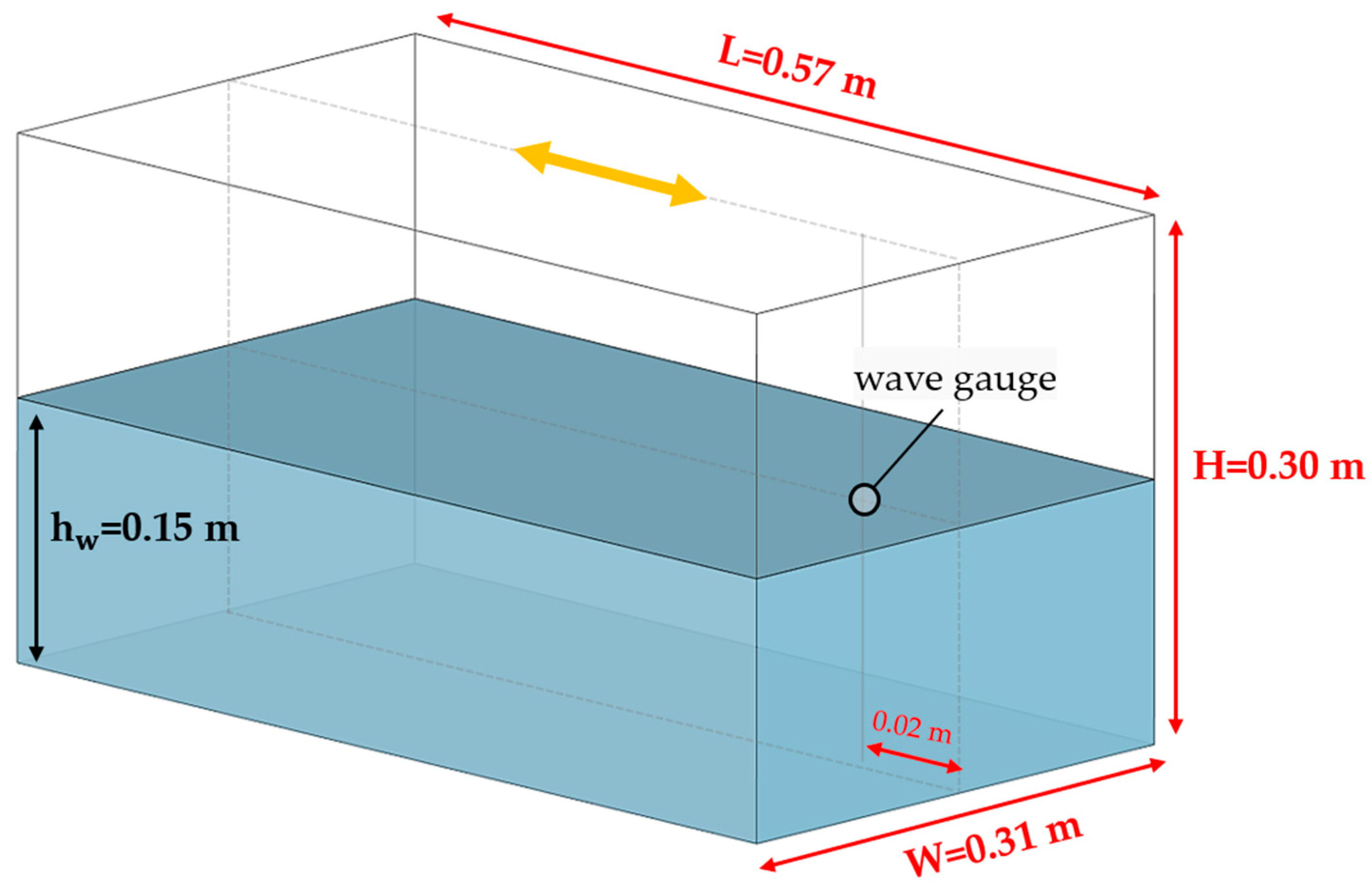
This section presents the results of a comparison between the numerical model used in this study and the experimental data from Liu and Lin (2020) [3] to validate the applied computational model. Figure 1 shows the dimensions of the 3D rectangular tank used in the experiment. The partially filled tank undergoes sinusoidal surge motion as described by Equation (1), induced by a shaker, and the free surface displacement is measured by a wave gauge positioned 0.02 m away from the wall.

When the water height is 0.15 m, the lowest natural sloshing frequency is 7.085 rad/s. For the validation test, the excitation frequency is set to $\omega ={\omega }_0$, and the excitation amplitude is A = 0.005 m.

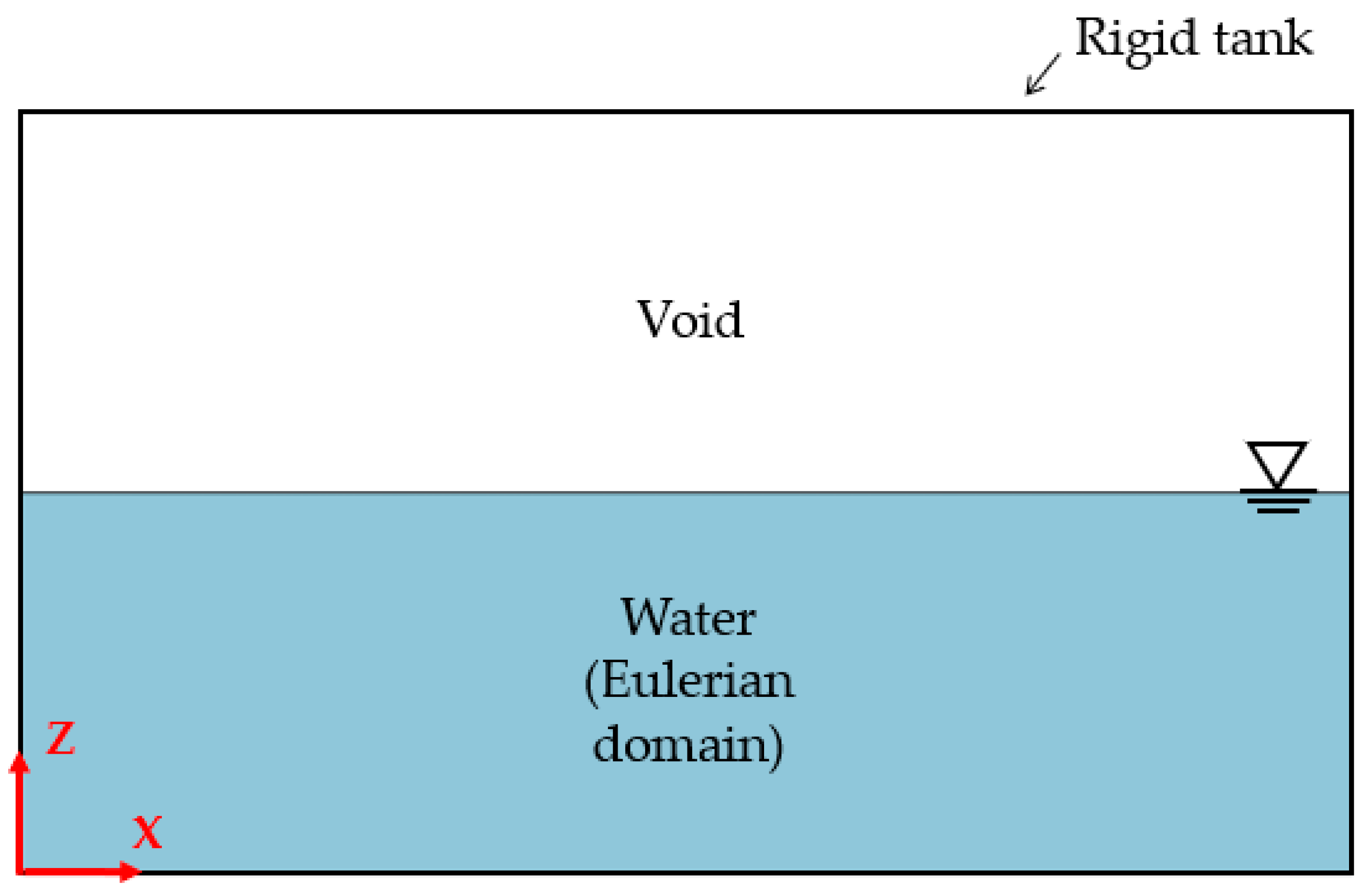
Figure 2 shows the schematic diagram of the finite element model used for the validation test. The numerical simulations were performed using the CEL module in the commercial software ABAQUS 2024. The tank is modeled using Lagrangian shell elements, with its deformation neglected. The water is modeled using Eulerian solid elements, while the regions outside the water are assigned to the void material option. For water simulation, the Us–Up EOS is applied. The EOS parameters implemented for the water are provided in

Table 1. Main particular and loading condition of the target structure.

Density (ρw) [kg/m3]	Dynamic Viscosity (η) [N∙s/m2]	Speed of Sound (c0) [m/s]	Γ0	s
1000	0.001	1450	0	0

.

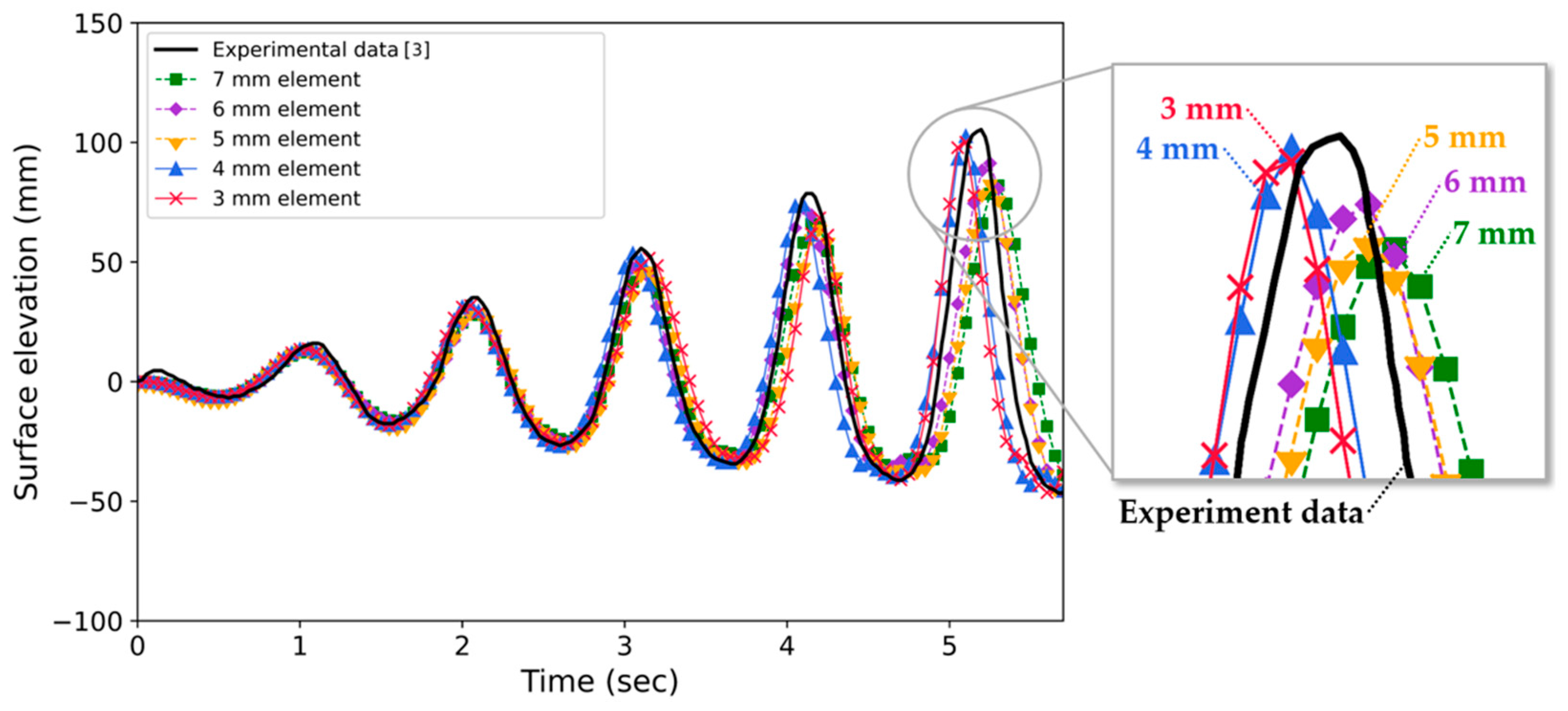
A mesh sensitivity study was conducted along with the validation test. The size of the Eulerian elements significantly affects the overall computation time, so simulations were performed with element sizes ranging from 3 mm to 7 mm to determine the optimized element size. Figure 3 shows snapshots of the free surface profile for each element size.

Figure 4 presents the results of the validation test. The simulation was run for approximately 6 s, with excitation applied at the calculated lowest natural sloshing frequency, enabling the observation of a clear resonant phenomenon. The results indicate that as the element size decreased, the simulation trend became more consistent with the experimental data, with convergence observed for element sizes smaller than 4 mm. To ensure higher accuracy, an element size of 3 mm was ultimately selected for this study.

4. Effect of Impulse Duration

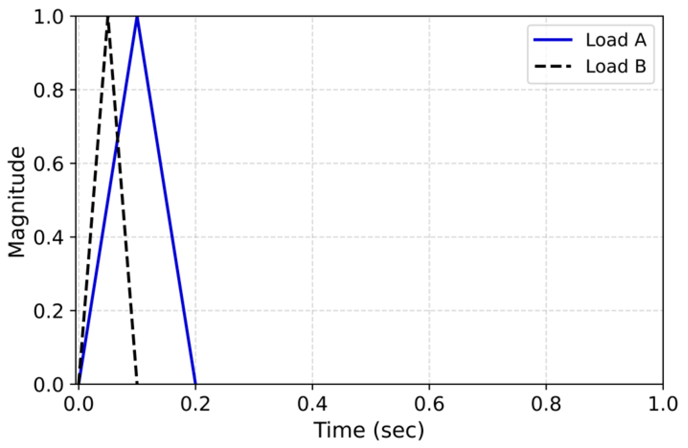
In this study, the IET is employed to identify the sloshing natural frequency of a water-filled tank. One of the key challenges in the numerical analysis of this method is the approximation of the Dirac delta function, which ideally represents an impulse applied over an infinitesimally short duration. However, in numerical simulations, a finite duration must be used to approximate the impulse.

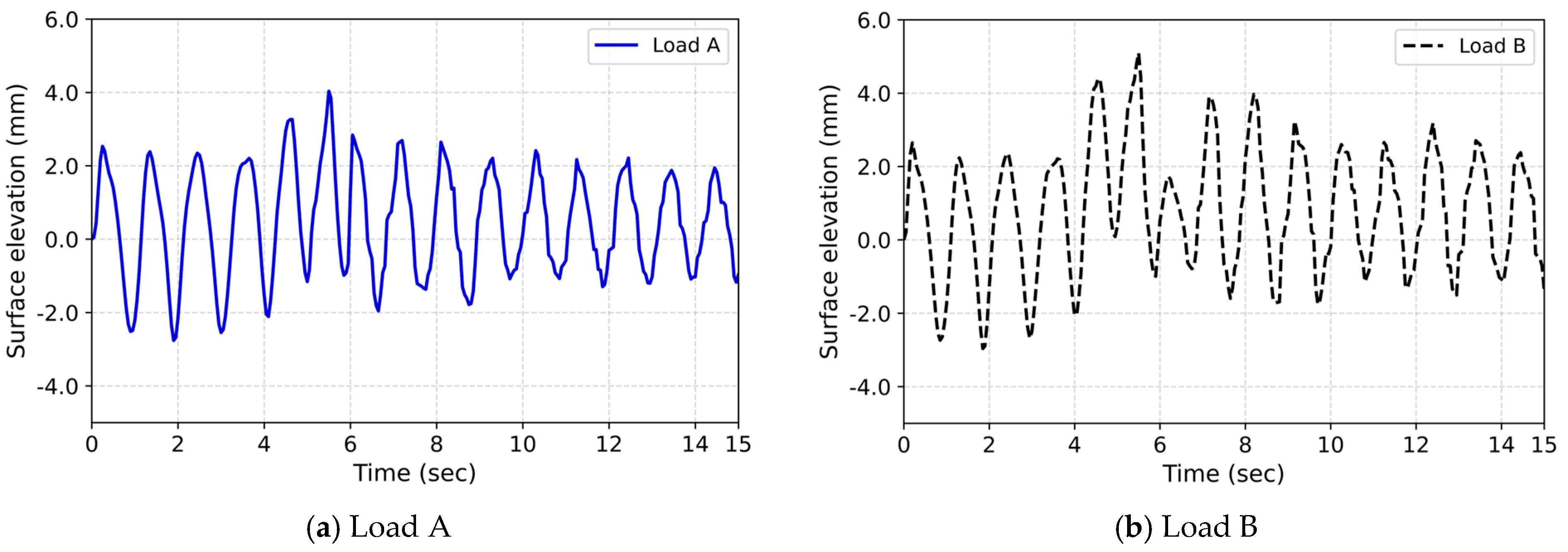
To evaluate the effect of impulse duration on the accuracy of the results, two cases with different rise times were considered. As shown in Figure 5, the first case involved an impulse with a rise time of 0.05 s, while the second case used a rise time of 0.1 s, which is twice as long as the first. Despite this difference, both rise times are still sufficiently short to effectively simulate an impulse excitation that closely approximates the ideal Dirac delta function, given the practical limitations of numerical methods and computational constraints.

Figure 6 presents the time-domain responses for both cases, while Figure 7 illustrates the corresponding Fourier Transform results. The frequency spectra indicate that both cases yield nearly identical peak frequencies and amplitudes, suggesting that the variation in rise time has minimal impact on the identified natural frequency.

5. Analysis Cases

In the case of a tank without baffles, the natural sloshing frequency closely matches the theoretical value derived from established formulas. Specifically, when the theoretically calculated natural frequency was used to model the tank, sloshing behavior was clearly observed, validating the theoretical approach. However, the situation becomes more complex when baffles are introduced. The presence of baffles alters the flow dynamics and, consequently, the sloshing frequencies, making it more challenging to predict the exact value of the natural frequency.

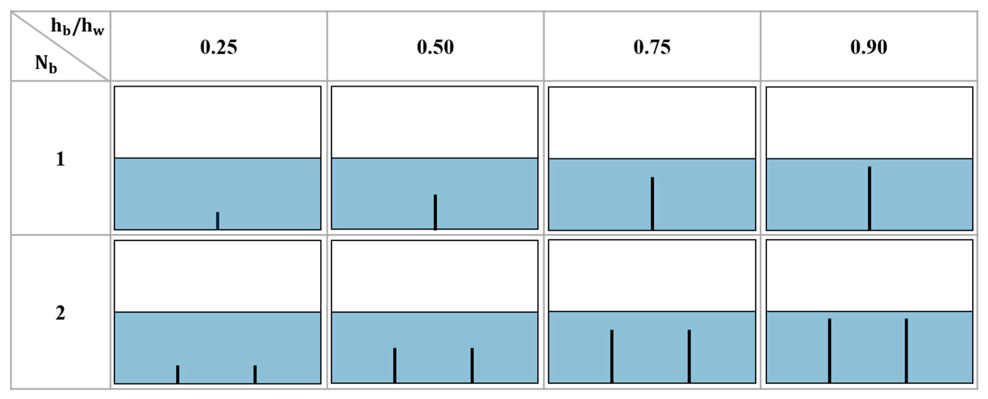
To investigate the impact of baffles on sloshing frequency, a detailed case study was conducted. This study considered a tank with one vertical baffle and a tank with two vertical baffles. Additionally, the baffle length was varied relative to the water depth, with lengths set at 25%, 50%, 75%, and 90% of the water depth. The analysis cases based on the number and length of baffles are summarized in Figure 8.

6. Analysis Results

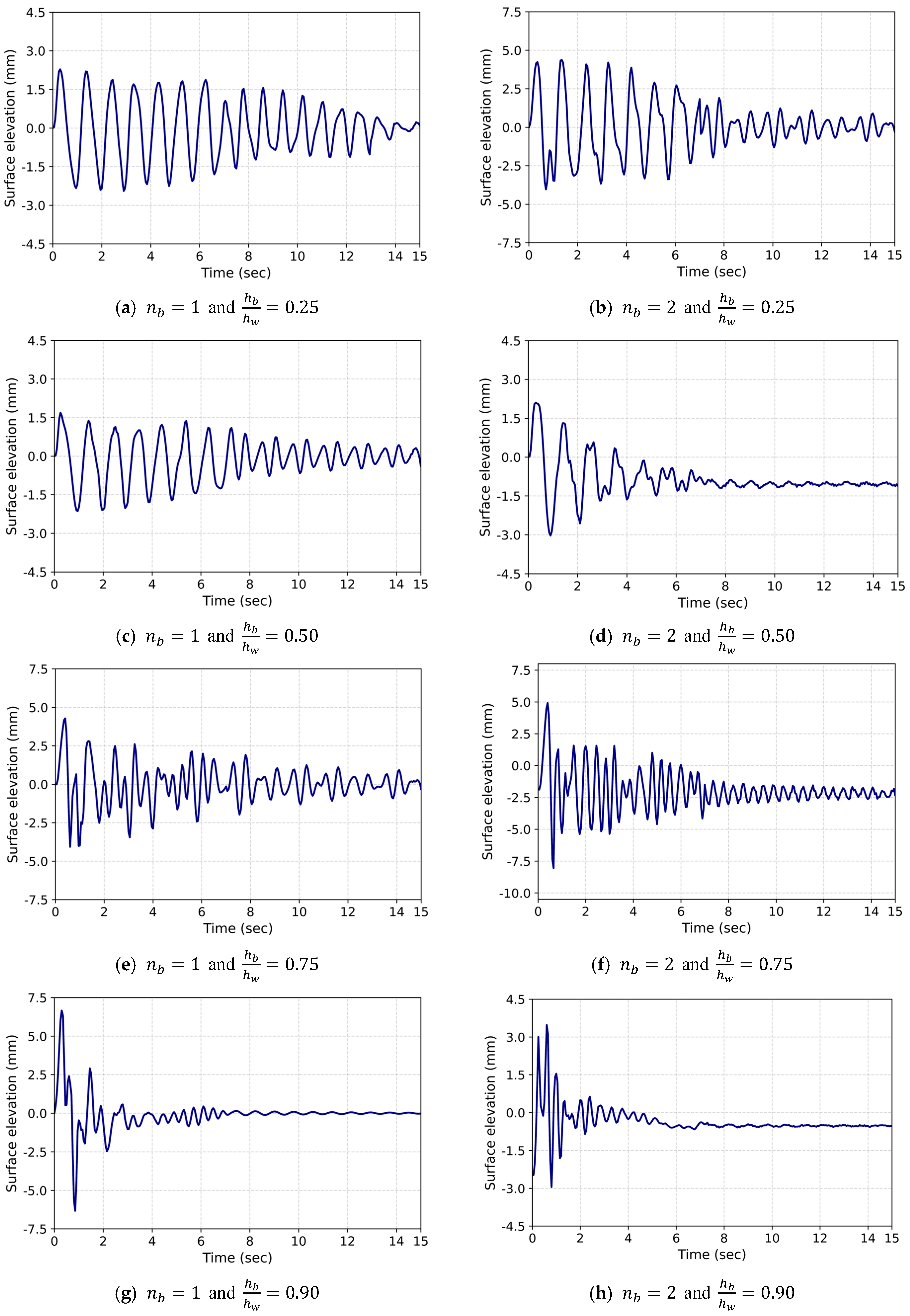
This section presents the results of numerical simulations performed by applying a unit impulse with a 0.05 s rise time to the cases summarized in Figure 8. As shown in Figure 1, the surface elevation was measured at a location 0.02 m away from the tank wall. The results from the 15 s simulation generally indicate that as the number of baffles increases from one to two, or as the baffle height increases, the vibrations decay more quickly as shown in Figure 9. This suggests that baffles play a significant role in controlling sloshing vibrations, with their effect becoming more pronounced as baffle height increases.

Figure 10 presents the frequency-domain results of the simulations, illustrating how the frequency characteristics vary depending on the number of baffles and their height. Specifically, the frequency response shapes remain similar for cases with two baffles at 50% height, but they begin to diverge once the baffle height exceeds 75%. This suggests that when the baffle height surpasses a certain threshold, its influence on fluid dynamics becomes nonlinear.

Figure 11 summarizes the lowest natural sloshing frequencies for each case. The results indicate that as the number of vertical baffles increases and their height rises, the lowest natural sloshing frequency consistently decreases. However, the trend differs depending on the number of baffles. For a single baffle, a sharp decrease in the lowest natural frequency occurs at ${\displaystyle \frac{h_b}{h_w}}=0.90$, whereas for two baffles, a significant drop is observed at a lower height ratio of ${\displaystyle \frac{h_b}{h_w}}=0.75$. A quantitative analysis of the nonlinear frequency shift shows that while the frequency decreases nearly linearly for lower baffle heights (${\displaystyle \frac{h_b}{h_w}}\le 0.50$), significant nonlinear deviations emerge at higher baffle heights. For a single baffle, the frequency deviation from the expected linear trend reaches approximately 5.0% at ${\displaystyle \frac{h_b}{h_w}}=0.75$ and increases sharply to about 20.8% at ${\displaystyle \frac{h_b}{h_w}}=0.90$. Similarly, for two baffles, the deviations are about 20.0% and 24.1% at ${\displaystyle \frac{h_b}{h_w}}=0.75$ and 0.90, respectively. These results quantitatively confirm that strong nonlinear effects arise when the baffle height exceeds approximately 75% of the water depth, especially in configurations with multiple baffles. Therefore, special attention must be paid when determining the natural sloshing frequencies of baffled tanks, as nonlinear effects can significantly alter the dynamic response.

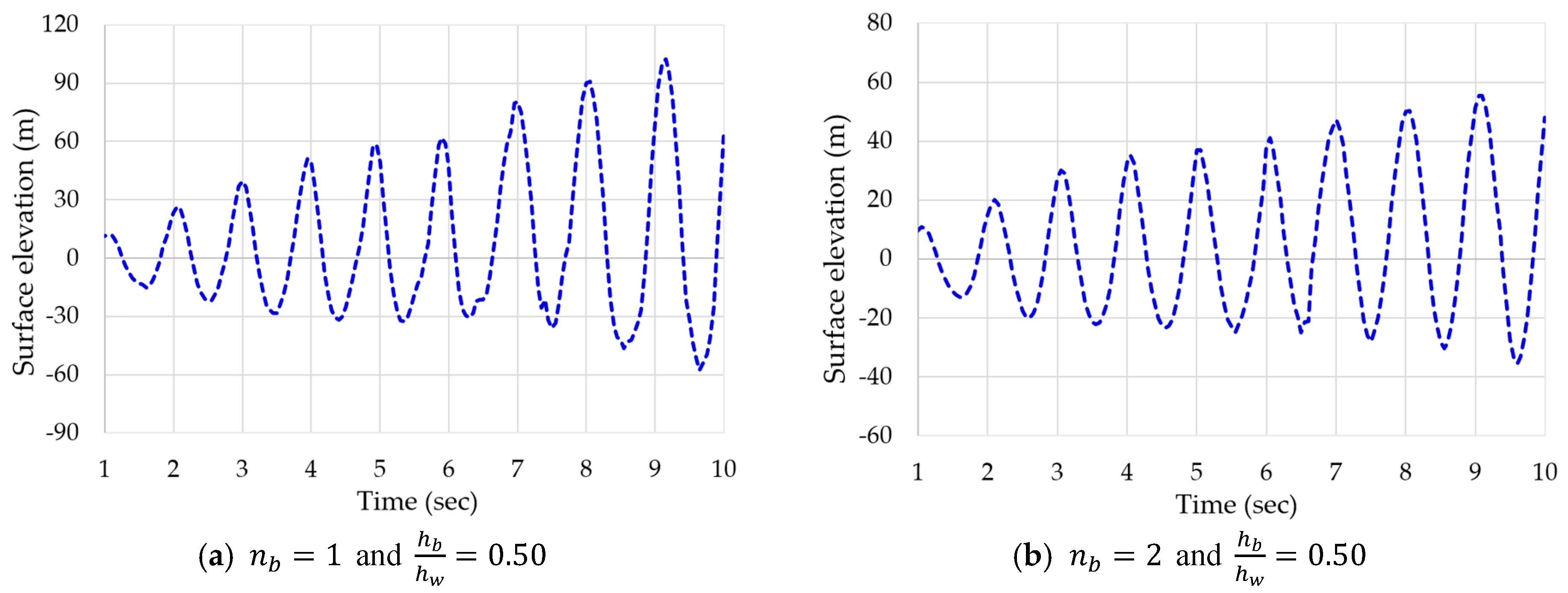
To validate the CEL-based calculations, a sloshing analysis was performed by applying the lowest natural frequencies summarized in Figure 11 to the target tank. The analysis was conducted for two cases: one with a single baffle at 50% height (see Figure 12a) and another with two baffles (see Figure 12b). The results show that a clear sloshing phenomenon was observed when the natural frequencies derived in this study were used for the analysis. As seen in Figure 4, for a tank without baffles, resonant phenomena were observed when the analysis was conducted using the natural frequencies calculated from the theoretical formula.

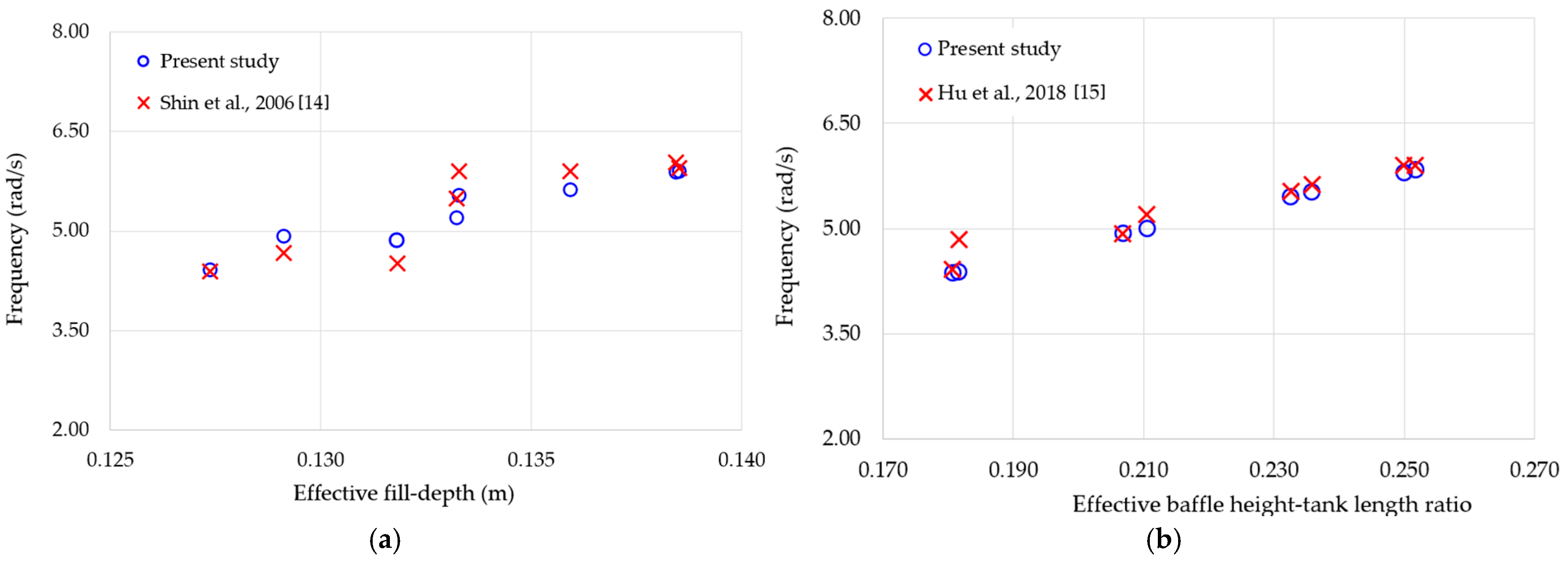
We compared the result of this study with the closed-form equations for the natural sloshing frequency of a tank with vertical baffles, as introduced in Section 2.1 (specifically, the equations by Shin et al. (2006) [16] and Hu et al. (2018) [17]). To compare with the equation from Shin et al. (2006) [16], we first calculated the effective fill-depth ($h_e$) based on the number and height of the baffles, and we then plotted the relationship between this effective fill-depth and the lowest natural sloshing frequency in Figure 13a. However, for comparison with the equation from Hu et al. (2018) [17], the effective baffle height-to-tank length ratio was calculated, and the results were plotted in Figure 13b.

To quantify the agreement, the root mean square error (RMSE) was calculated separately for each model. The RMSE between the numerical results and Hu et al. (2018) [17] was 0.25 rad/s, while the RMSE for Shin et al. (2006) [16] was 0.19 rad/s. When compared to the average values of the natural sloshing frequencies, these RMSE values correspond to relative errors of about 4.5% and 3.5%, respectively. Since both values are well below 5%, they indicate a good level of agreement between the numerical and theoretical results.

However, this similarity may be attributed to the comparison being limited to only the lowest natural frequency. If higher-order natural sloshing frequencies were also analyzed, more noticeable differences might emerge. Therefore, conducting further studies that calculate and compare higher-order frequencies would be valuable for gaining a more comprehensive understanding of the discrepancies.

Additionally, the IET method used in this study proved to be effective in determining the sloshing natural frequencies through numerical simulations. Applying this method experimentally in further studies is expected to make significant contributions to research focused on identifying sloshing natural frequencies more accurately.

7. Discussion

This study investigated the impact of vertical baffles on the natural sloshing frequencies of a rectangular tank using the CEL method in combination with the IET. The results demonstrated that both the number and height of baffles significantly influence the dynamic behavior of the fluid. In tanks without baffles, the computed natural frequencies closely matched theoretical predictions, validating the applicability of traditional analytical models under simplified conditions.

As the number or height of baffles increased, the natural frequencies decreased. This shift is attributed to the reduction in effective free surface area and the disruption of coherent sloshing paths caused by internal barriers. When the baffle height exceeded approximately 75% of the water depth, the fluid domain became segmented, resulting in localized vortex formation and entrapped fluid zones. These effects introduced nonlinearities in the fluid motion, leading to deviations from linear theoretical predictions.

A key contribution of this study is the comparison of numerically obtained natural frequencies with closed-form solutions proposed by Shin et al. (2006) [16] and Hu et al. (2018) [17]. Although good agreement was observed for the fundamental mode, the comparison was limited to this lowest frequency. Closed-form models, based on linear assumptions and two-dimensional simplifications, are insufficient to capture the three-dimensional flow structures and nonlinear phenomena introduced by tall or multiple baffles. In contrast, the CEL-based approach effectively accounts for such complexities, demonstrating its value in sloshing analysis for baffled tanks.

The CEL method also offers the advantage of directly simulating fluid–structure interaction without simplifying the governing equations. This enables accurate modeling of key flow phenomena such as large free surface deformation, vortex shedding, and flow separation, features essential for understanding sloshing behavior in the presence of internal structures.

In this study, the tank walls and baffles were assumed to be rigid, neglecting structural deformation under fluid-induced loads. While this assumption is valid for stiff-walled tanks, it may not apply to flexible or lightweight structures, where structural compliance can alter the fluid response. Future studies should address this limitation by implementing fully coupled fluid–structure interaction (FSI) models.

The analysis focused primarily on the fundamental sloshing mode. Higher-order modes, which may respond differently depending on baffle configuration and potentially interact with structural modes, were not examined in detail. Such interactions could lead to complex dynamic behaviors including mode coupling and resonance. Comprehensive modal analysis, including frequency shifts and damping characteristics, will be essential to fully characterize the dynamic response of baffled fluid systems. In this context, distinguishing true physical behavior from numerical artifacts is critical for ensuring the reliability of simulation results.

In addition, the present study was limited to rectangular tanks with vertical baffles. In practice, sloshing behavior can vary significantly with tank geometry, such as cylindrical, spherical, or irregular shapes, and the spatial arrangement of internal components. Future work should extend the proposed framework to a broader range of tank configurations to evaluate its robustness and general applicability.

Lastly, as this study was based solely on numerical simulations, experimental validation is essential to confirm the accuracy and practical relevance of the findings. Real-world factors such as structural imperfections, measurement noise, and external disturbances should be incorporated into future experimental investigations.

In summary, this study provides valuable insights into how vertical baffles affect sloshing dynamics and shift of natural frequencies. To improve the generalizability and predictive performance of the proposed modeling framework, future research should incorporate higher-order modes, structural flexibility, experimental validation, and a wider range of tank geometries and internal configurations.

8. Conclusions

This study introduced an integrated numerical framework for predicting natural sloshing frequencies in baffled rectangular tanks, combining the CEL method with the IET. The results demonstrate that vertical baffles significantly alter the fluid’s dynamic behavior, primarily by reducing natural frequencies and introducing nonlinear flow features, particularly when the baffle height exceeds a critical threshold relative to water depth.

This study also revealed that when the baffle height exceeds a certain threshold, the sloshing behavior exhibits nonlinear characteristics, leading to a significant shift in the frequency response. This nonlinearity is crucial for understanding the full range of sloshing behavior in baffled tanks, which is often not adequately captured by traditional theoretical models.

Through a comparison with the closed-form equations developed by Shin et al. (2006) [16] and Hu et al. (2006) [17], this study demonstrated that with regard to the lowest natural sloshing frequency, the closed-form equations based on the potential theory can yield reasonable results when applied to tanks with vertical baffles. Also, the CEL-IET method proved to be a reliable framework for modeling and predicting sloshing behavior in complex tank geometries.

Despite these contributions, this study has several limitations. The analysis was restricted to the fundamental mode; higher-order sloshing modes and their possible interactions with structural modes were not addressed. The tank and baffles were modeled as rigid structures, neglecting the effects of structural flexibility. In addition, only rectangular tank geometries were considered, whereas sloshing dynamics can vary considerably across different tank shapes and internal layouts.

Furthermore, since the findings are based solely on numerical simulations, experimental validation is essential. Real-world factors such as fabrication tolerances, external disturbances, and measurement uncertainties must be accounted for to assess the practical applicability of the proposed method.

Future research should therefore focus on the following areas:

-

Extending modal analysis to capture higher-order sloshing frequencies and their interactions;

-

Implementing fully coupled fluid–structure interaction (FSI) modeling for flexible structures;

-

Applying the method to a broader range of tank geometries and baffle configurations;

-

Conducting experimental studies to validate and refine the simulation results.

By addressing these aspects, the proposed framework can be further advanced into a predictive and generalizable tool for the design and safety evaluation of liquid-containing structures in marine, aerospace, automotive, and energy industries.