Predicting Cardiovascular Aging Risk Based on Clinical Data Through the Integration of Mathematical Modeling and Machine Learning

Abstract

Background: The aging population is increasing rapidly, with individuals aged 65 and older now representing more than 15% of the global population. This demographic shift is associated with a rising incidence of age-related cardiovascular diseases (CVDs). Early prediction and prevention of cardiovascular aging are essential to improve health outcomes among elderly patients. Objective: This study aimed to develop and externally validate a mathematical model for predicting cardiovascular aging in individuals aged 65 and older, based on general clinical and behavioral data. Methods: The model was built using data from 800 individuals aged 65+ from Almaty, Kazakhstan. Predictors included sex, marital status, education, smoking, alcohol use, disability, physical activity, total cholesterol, hypertension, BMI, coronary artery disease (CAD), myocardial infarction, diabetes mellitus, and chronic heart failure. A system of ordinary differential equations was used to simulate the dynamic interactions of these factors. Numerical integration was performed using the Runge–Kutta, Adams–Bashforth, and backward Euler methods. The model was verified statistically using Pearson correlation analysis and externally validated on independent age cohorts. In addition, we applied k-means clustering to identify hidden patterns and risk profiles within the dataset. A Random Forest classifier was trained to distinguish between high-risk and low-risk individuals using the same feature set. These machine learning approaches were used as complementary tools to enhance the robustness and interpretability of the modeling results. Results: The model trained on the 65–74 age group achieved an external validation accuracy of 98.8% and an AUC of 0.989 when applied to the 75–89 group. Risk modeling showed that in the 65–74 group, smoking and alcohol increased the risk of myocardial infarction, hypertension, and obesity by up to 53%. In the 75–89 group, these factors increased the likelihood of hypertension by 21%, chronic heart failure by 16%, and CAD by 14%. Among individuals aged 90+, hypercholesterolemia increased the risk of chronic heart failure by 17%, while hypertension increased myocardial infarction risk by 16%. Conclusions: The proposed model demonstrated high accuracy in predicting cardiovascular aging and identifying high-risk individuals across elderly subgroups. The integration of clustering and classification methods (k-means and Random Forest) provided additional insights and confirmed the consistency of the findings. This multi-method approach may serve as a valuable tool for developing personalized prevention strategies in geriatric care and improving healthy life expectancy.

1. Introduction

Cardiovascular disease (CVD) is one of the leading causes of morbidity and mortality among older people worldwide. The risk of CVD increases significantly with age, which makes early detection and prediction of the progression of cardiovascular aging particularly important [1,2]. Modern methods of diagnosis and treatment can significantly improve the quality of life of patients, but in order to optimize treatment strategies, it is necessary to understand how various physiological and behavioral factors influence the process of cardiovascular aging. According to worldwide studies, a correlation between aging and many factors, such as lifestyle, nutrition, gene polymorphisms, immune inflammation, endothelial dysfunction, and others, has been identified [3]. However, the identification of the relationship between these factors in individuals subjected to accelerated cardiovascular aging in the population of Kazakhstan still requires additional scientific research.

The preventive direction in cardiology is based on the strategy of early detection of persons at high risk of cardiovascular diseases. Mathematical modelling is a powerful tool for analyzing complex biological systems and predicting their dynamics. In recent years, mathematical modeling methods have been actively used in medicine to study various diseases and develop individualized approaches to treatment. In particular, models based on differential equations and probabilistic methods allow taking into account multiple interacting factors and making long-term predictions.

Existing prediction approaches include the use of biomarkers. To create a mathematical model in our work, various social/behavioral factors and clinical data were selected as biomarkers to study cardiovascular ageing of respondents: gender, marital status, education, smoking, alcohol consumption, disability, physical activity, total cholesterol, arterial hypertension, body mass index, CHD, myocardial infarction, diabetes mellitus, chronic heart failure.

The development of mathematical modelling in medicine and experimental scientific work is actively considered in the modern scientific community. The scales used to determine the risk of cardiovascular events are aimed at preventing and predicting cardiovascular mortality and non-fatal events. The SCORE (Systematic COronary Risk Evaluation) scale assesses the risk of death from cardiovascular disease over the next 10 years, and improved scales are used to predict the 10-year risk of fatal and non-fatal cardiovascular events in people aged 40–69 (SCORE2) and older than 70 years (SCORE2-OP). The indicators are age, sex, smoking, blood pressure, and cholesterol. However, these risk scales have several limitations: a lack of accuracy for an individual or the appearance of “residual risk” [4].

Polo Y La Borda et al. [5] evaluated the prognostic value of four cardiovascular (CV) risk algorithms, SCORE, its modified version (mSCORE), European Alliance of Rheumatological Associations (EULAR) 2015/2016, SCORE2 algorithm (updated and improved version of SCORE), and QRESEARCH risk assessor version 3 (QRISK3), to identify high-risk patients in a group of individuals with psoriatic arthritis. The four cardiovascular risk scales showed strong correlations, and all of them showed a significant association with cardiovascular events (p < 0.001). Risk diagram algorithms were very useful for distinguishing PsA at low and high cardiovascular risk. The integrated model with QRISK3 and SCORE2 gave an optimal synergy between the discriminative power of QRISK3 and the calibration accuracy of SCORE2.

The present work aimed to develop and validate a mathematical model to predict cardiovascular aging in people aged 65 years and older.

The use of our model will allow us not only to predict the progression of cardiovascular aging but also to identify patients at increased risk of CVD, which will open new opportunities for prevention and early intervention.

The issues of the development of mathematical models in medicine and experimental scientific works are actively considered in the modern scientific community. Marokov’s study [6] is devoted to a simple mathematical model of aging based on a system of autonomous ODEs of the first order. The key assumption of the model is that the organism has no internal clock counting down chronological time on the scale of decades. Instead, the organism uses internal biological factors denoted by variables g_i(t), each of which counts down its biological time t_i. Overall, the proposed model provides a simple and efficient framework for systematizing experimental data on age-related changes in different biological subsystems of an organism. Even in linear approximation, the parameters {a_i, b_ij} allow us to quantitatively identify and structure the significant cause-and-effect relationships for the aging process.

Murase et al. represent the aging process using a one-dimensional model of a multicellular system that allows the analysis of local and global modes of cell behavior [7]. In the early stages, simple interactions provide coordinated patterns, whereas in later stages, complex interactions result in chaotic changes reflecting an abnormal state.

In the study [8], the complex cellular mechanisms that characterize aging are reviewed with a focus on two metabolic centers: mTOR and NAD+-dependent deacetylase SIRT1. Experimental evidence points to an interaction between these pathways, but the mechanisms of their interaction remain unclear. The authors propose to use computational modelling combined with experiments to elucidate these mechanisms. The basic models are discussed and a reduced reaction pathway for modelling is presented. Finally, the limitations of computational modelling and opportunities for future research in this area are described. The main limitation of the approach is the need for a precise set of parameters. Therefore, well-studied areas should be modelled first to gradually understand the mechanisms and develop new therapies to increase healthy life expectancy or slow aging. Moreover, in [9], a mathematical model describing the influence of the environment on the aging of living systems is presented. It is based on the competition between the destruction and restoration of a biological system regulated by the kinetics of autocatalytic reactions. The influence of the environment is considered through time-dependent parameters corresponding to thermodynamic and gerontological principles, as well as medical observations.

Hibs [10] discusses mathematical models of physiological behavior that describe a system returning to the initial state after a perturbation through homeostasis. These models include the concept of a “fatal limit” of system deviation. The author concludes that the numerical values of the limits depend on other parameters, such as recovery times and coupling coefficients, and can be experimentally measured. Age-related changes in parameters and the derivation of mortality parameters, such as Gompertz parameters, from experimental data are discussed.

The process of proliferative cell senescence in culture has been described using a mathematical model [11]. Based on the hypothesis of DNA damage as a cause of cell senescence, the model can explain both limited and unlimited proliferative potential of both normal and transformed cells in vitro. According to the model, the fate of a cell population depends on two counteracting factors: the rate of proliferation of dividing cells and the rate of accumulation of gene damage. Computer simulations demonstrate agreement with experimental data in general terms.

Based on Rifin’s mathematical model, a 10-year cardiovascular disease (CVD) risk estimate using the WHO scale was presented in [12] using data from 5503 adults in Malaysia. It was found that 4.9% of participants had a high risk (≥20%), which was more common in males (7.3%) compared to females (2.5%). Major risk factors included low education level, unemployment, and obesity combined with physical inactivity (aOR = 2.19). The recommended interventions to reduce risk included health promotion, screenings and information campaigns. These results highlight the importance of targeted prevention programs for high-risk groups.

A large-scale study [13] used data from 10,432 individuals aged 40 to 69 years to compare 17 measures of adiposity (ROC) to predict arterial hypertension and dyslipidemia, which are major predictors of cardiovascular disease, type 2 diabetes (T2DM), and multimorbidity. ROC and logistic regression curves showed that the Chinese visceral adiposity index (CVAI) and triglyceride-glucose index (TYG) better predicted arterial hypertension and multimorbidity, and body mass index (BMI) better predicted dyslipidemia.

Personalized prediction of cardiovascular disease using multi-omics technologies and machine learning techniques was conducted in a study [14] that combined RNA sequencing data, single nucleotide polymorphisms (SNPs), and clinical information to create personalized risk profiles. Using trait selection methods, researchers identified 27 key transcriptomic markers and SNPs that distinguished patients with cardiovascular disease. An optimized XGboost model tuned with Bayesian hyperparameters demonstrated high accuracy. Risk assessment using Shapley’s additive mixture helped to explain the importance of biomarkers (RPL36AP37 and HBA1), which was supported by the literature and demonstrated the potential of the framework to predict other diseases.

An epidemiological study of cardiovascular disease (CVD) in Kashgar Prefecture, Xinjiang, northwest China was conducted to identify key risk factors. Data from 1,887,710 adults (baseline 2017) from the Kashgar prospective cohort study were analyzed, including 16 potential factors—7 demographic, 4 lifestyle, and 5 clinical factors—collected through questionnaires and medical examinations. Logistic regression models showed that all factors were significantly associated with SWD (odds ratio 1.03 to 2.99, p < 0.05). Machine learning methods (Random Forest, Random Ferns, Extreme Gradient Boosting) ranked age, occupation, hypertension, exercise frequency, and dietary patterns as the five major risk factors for SWD. Stratification analyses showed consistent rankings across subgroups. This study considered cardiovascular disease as a major problem in Kashgar, and these five factors were crucial for future preventive measures [15].

A recent study [16] explored the interplay between SARS-CoV-2 (SC-2) transmission and cardiovascular complications, particularly heart attacks, using advanced mathematical modeling. A fractional-order system incorporating a fractal fractional operator (FFO) was employed to analyze local and global stability through Lyapunov functions and flip bifurcation testing. Key epidemic properties, including existence, boundedness, and positivity, were examined to ensure reliable findings. Simulations highlighted symptomatic and asymptomatic effects, offering insights into the combined impact of SC-2 and cardiovascular conditions. These approaches contributed to a deeper understanding of disease dynamics and informed future prediction and control strategies.

Another study [17] focused on fractional-order modeling of cholera transmission, incorporating both asymptomatic cases and treatment interventions. The Atangana–Toufik scheme was applied to examine the system’s stability, boundedness, and bifurcation properties, confirming the absence of flip bifurcation. The reproductive number (R₀;) was computed to evaluate the transmission potential, while a sensitivity analysis highlighted key factors affecting disease spread. MATLAB R2024a simulations illustrated the role of asymptomatic measures and treatment in controlling the outbreak. These insights enhanced the understanding of cholera dynamics, supported early detection efforts, and contributed to the development of effective disease control strategies.

2. Materials and Methods

Problem statement: The determination of biomarkers for the mathematical model of cardiovascular aging prediction was based on their clinical significance and confirmed role in the development of cardiovascular diseases (CVD). The study included data from 800 people aged 65–74, 75–89, and 90+ (see Figure 1) according to the WHO classification. Questionnaires were administered using four standard international questionnaires, which ensured comprehensive collection of information on risk factors.

The weights of individual biomarkers were assigned based on their clinical relevance and alignment with modifiable or non-modifiable cardiovascular risk factors, in accordance with international recommendations. Modifiable factors included dyslipoproteinemia, arterial hypertension, diabetes mellitus, smoking, physical activity, and obesity, as they were directly related to the progression of vascular aging and can be corrected by preventive strategies. Non-modifiable factors, such as gender and age, were included in the model because they determined the baseline risk level and influenced the body’s response to external influences.

Factor weights were determined using statistical analysis and machine learning methods. A correlation analysis (Pearson’s coefficients) allowed us to identify the degree of association of each factor with the processes of cardiovascular aging. Numerical modelling using Runge–Kutta, Adams–Bashforth and backward Euler methods allowed us to describe the dynamic interaction of risk factors over time.

Thus, the included biomarkers reflected the key mechanisms of cardiovascular aging, and their weights in the model were determined taking into account evidence and a complex statistical analysis, providing high accuracy of prediction and the possibility of individualized prevention.

To create the mathematical model, the following parameters were selected as biomarkers of cardiovascular ageing and social status of the respondents, which had high Pearson correlation values:

ch is cholesterol (total cholesterol);

Pr is blood pressure (hypertension);

W is body mass index (BMI);

Px is postinfarction cardiosclerosis;

X is chronic heart failure (CHF);

G is gender;

S is smoking;

E is education;

A is alcohol;

I is ischemic heart disease (IHD).

$a_1$, $b_1$, $c_1$, $d_1$, $a_2$, $b_2$, $c_2$, $d_2$, $a_3$, $b_3$, $c_3$, and $d_3$ are constants. These markers were selected as the best results when calculating the Pearson correlation coefficient from the biomarker statistics of the experimented patients:

$$r={\displaystyle \frac{{\sum }_{i=1}^N\left(x_i-\overline{x}\right)\left(y_i-\overline{y}\right)}{\sqrt{{\sum }_{i=1}^N{\left(x_i-\overline{x}\right)}^2}\sqrt{{\sum }_{i=1}^N{\left(y_i-\overline{y}\right)}^2}}}$$

(1)

Here, r is the correlation coefficient, x_i are clinical biomarkers, y_i are social parameters, $\overline{y}$ is the mean value of clinical biomarkers, $\overline{y}$ is the mean value of social parameters, and N is the number of biomarkers and parameters that match.

3. Results and Discussion

All actual values of the database were dimensionless (by dividing the value of each column by the maximum value of the same column). Dimensionless values bring all values to the interval from zero to one. This procedure makes the equation less rigid and simplifies the computational process. In this paper, all values were dimensionless.

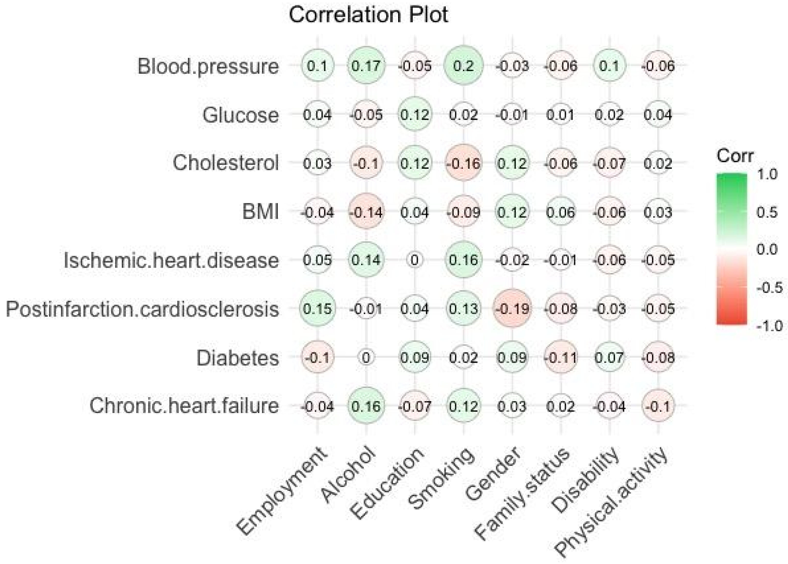
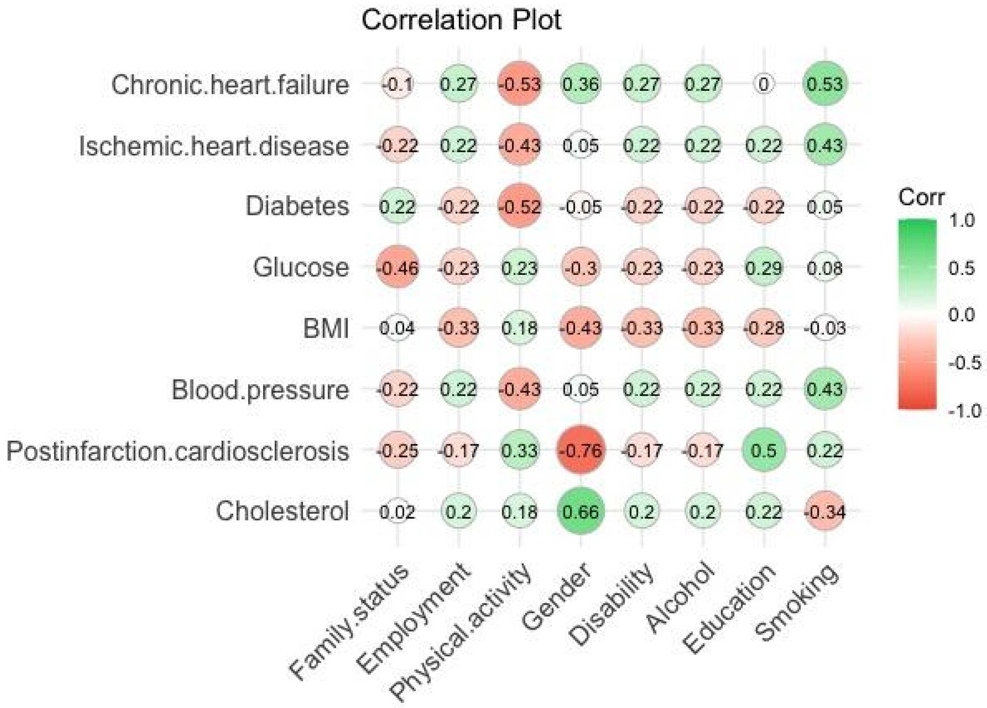
Pearson’s correlation coefficients were calculated according to Formula (1), which characterize the strength of the relationship between the parameters (≤1). The results of calculating the correlation between the biomarkers and social characteristics of respondents are shown in Figure 2, Figure 3 and Figure 4:

From the correlation plots (see Figure 2, Figure 3 and Figure 4), we determined the best relationships between biomarkers and social characteristics of respondents to show the level of interaction between the product of parameters in Equations (2)–(4) as shown in

Table 1. Coefficients of the mathematical model.

Age Category	Coefficient	Value
65–74	$a_1$	0.66
	$b_1$	0.53
	$c_1$	0.5
	$d_1$	0.43
74–89	$a_2$	0.21
	$b_2$	0.15
	$c_2$	0.16
	$d_2$	0.14
90+	$a_3$	0.17
	$b_3$	0.17
	$c_3$	0.16
	$d_3$	0.16

.

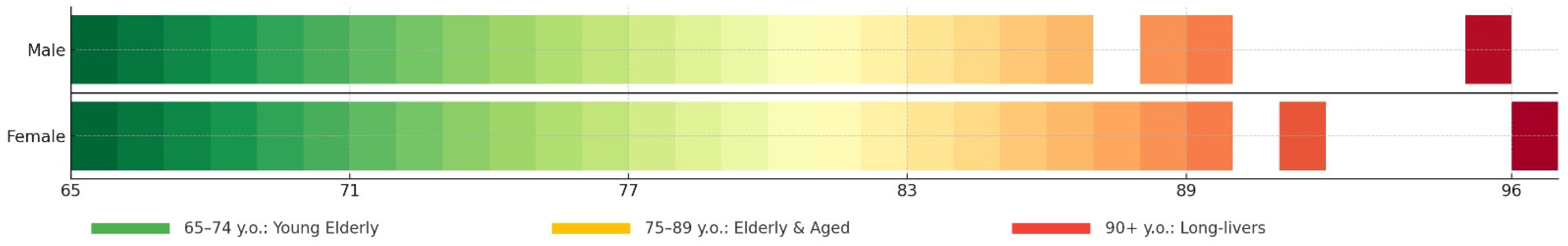
We developed a mathematical model in the form of a nonlinear dynamic (nonstationary) equation that could provide a prediction of changes in premature aging. For patients in the age range of 65–74 years, we mathematically assumed that their cardiovascular system aged as follows:

$${\displaystyle \frac{dx}{dt}}=a_1·Px\left(x,t\right)·S\left(x,t\right)+b_1·Px\left(x,t\right)·A\left(x,t\right)+c_1·I\left(x,t\right)·S\left(x,t\right)+d_1·Pr\left(x,t\right)·S\left(x,t\right),$$

(2)

where the total derivative ${\displaystyle \frac{dx}{dt}}$ in the left part of Equation (2) represents the process of premature ageing by time t. The first term is the interaction of postinfarction cardiosclerosis and smoking, the second term postinfarction cardiosclerosis and alcohol, the third term body mass index with smoking, and the fourth term blood pressure with smoking, respectively, with probabilities $a_1$, $b_1$, $c_1$, and $d_1$.

Cardiovascular aging for patients in the age range 75–89 could be described as the following differential equation:

$${\displaystyle \frac{dx}{dt}}=a_2·Pr\left(x,t\right)·S\left(x,t\right)+b_2·Pr\left(x,t\right)·A\left(x,t\right)+c_2·X\left(x,t\right)·A\left(x,t\right)+d_2·I\left(x,t\right)·S\left(x,t\right),$$

(3)

where ${\displaystyle \frac{dx}{dt}}$ represents changes in premature aging over time t, the first and second terms are the interactions of blood pressure with smoking and alcohol, the third term chronic heart failure with alcohol, and the fourth ischemic heart disease with smoking, respectively, with probabilities $a_2$, $b_2$, $c_2$, and $d_2$.

$a_1$, $b_1$, $c_1$, $d_1$, $a_2$,$b_2$, $c_2$, and $d_2$ are interaction coefficients of the indicated markers. The derivatives of biomarkers in Equations (2) and (3) were chosen in such a way that they showed the best correlation relations.

Thus, as a result, in Equations (2) and (3) of the mathematical model of premature aging of people in the age intervals 65–74 and 75–89, it can be observed that smoking and alcohol are present in all products of biomarkers, which indicates high correlation. Smoking and alcohol consumption in these age intervals can lead to postinfarction cardiosclerosis, coronary heart disease, variation in blood pressure, and changes in blood cholesterol levels. It can be concluded that people in this age range should give up bad habits in order to maintain and prevent their decline in biological age.

Cardiovascular aging for patients aged 90+ was described as follows:

$${\displaystyle \frac{dx}{dt}}=a_3·G\left(x,t\right)·ch\left(x,t\right)+b_3·S\left(x,t\right)·X\left(x,t\right)+c_3·Px\left(x,t\right)·E\left(x,t\right)+d_3·Pr\left(x,t\right)·S\left(x,t\right),$$

(4)

where ${\displaystyle \frac{dx}{dt}}$ is the time derivative of cardiovascular aging and means changes in premature aging through time t, $a_3$ is the value of the correlation coefficient of the interaction between human sex and chronic heart failure, $b_3$ is the value of the correlation coefficient of the interaction between smoking and cholesterol, $c_3$ is the value of the correlation coefficient of the interaction between postinfarction cardiosclerosis and human education, and $d_3$ is the value of the correlation coefficient of the interaction between blood pressure and smoking.

The choice of the product of parameters in Equation (4) refers to their high correlation values. The first product shows the interactions and dependence of cholesterol level on human gender (women in this age group are more likely to have elevated cholesterol levels). From the second product, we can conclude that smoking can lead to chronic heart failure. The third product selected from the correlation results shows that a person’s social status as an entity may influence the development of myocardial infarction. The assumption here is that education can lead a person to psychological resilience, which may prevent postinfarction cardiosclerosis. The fourth product shows that smoking leads to a variation in blood pressure. Moreover, the addition of the products means that the interactions of other pairs of biomarkers also showed good correlation results, and their level of interaction is described by the coefficients $a_3$, $b_3$, $c_3$, and $d_3$.

The parameters $Px\left(x,t\right)$, $A\left(x,t\right)$, $I\left(x,t\right)$, $Pr\left(x,t\right)$, $S\left(x,t\right)$, $X\left(x,t\right)$, $G\left(x,t\right)$, $ch\left(x,t\right)$, and $E\left(x,t\right)$ used for calculating the correlation coefficient were read from the statistical database. The initial conditions were as follows:

$Px\left(x,0\right)=0$, $A\left(x,0\right)=0$, $I\left(x,0\right)=0$, $Pr\left(x,0\right)=0$, $S\left(x,0\right)=0$, $X\left(x,0\right)=0$, $G\left(x,0\right)=0$, $ch\left(x,0\right)=0$, $E\left(x,0\right)=0$.

The first boundary conditions were as follows:

$Px\left(0,t\right)=1$, $A\left(0,t\right)=1$, $I\left(0,t\right)=1$, $Pr\left(0,t\right)=1$, $S\left(0,t\right)=1$, $X\left(0,t\right)=1$, $G\left(0,t\right)=1$, $ch\left(0,t\right)=1$, $E\left(0,t\right)=1$.

For the numerical solution of Equations (2)–(4), these parameters have the following expressions:

$$\begin{array}{c}Px\left(x,t\right)=Px\left(x-1,t\right)+i∆x,\\ A\left(x,t\right)=A\left(x-1,t\right)+i∆x,\\ I\left(x,t\right)=I\left(x-1,t\right)+i∆x,\\ Pr\left(x,t\right)=Pr\left(x-1,t\right)+i∆x,\\ S\left(x,t\right)=S\left(x-1,t\right)+i∆x,\\ X\left(x,t\right)=X\left(x-1,t\right)+i∆x,\\ G\left(x,t\right)=G\left(x-1,t\right)+i∆x,\\ ch\left(x,t\right)=ch\left(x-1,t\right)+i∆x,\\ E\left(x,t\right)=E\left(x-1,t\right)+i∆x,\end{array}$$

with $∆x={\displaystyle \frac{b-a}{N}}$ the grid spacing. However, in order to obtain previous values, the parameters had their values taken from the statistical database.

For numerical modeling, the fourth-order Runge–Kutta method [18], Adams–Bashforth method [19], and backward Euler method [20] were used to solve ordinary differential Equation (4). First, we considered the fourth-order Runge–Kutta method:

$$x\prime =a_3·G\left(x,t\right)·ch\left(x,t\right)+b_3·S\left(x,t\right)·X\left(x,t\right)+c_3·Px(x,t)·E(x,t){+d}_3·Pr(x,t)·S(x,t),$$

where $x\left(t\right)$ is the right part of Equation (4).

The finite solution of the ODE by the Runge–Kutta method is:

$$x_{n+1}=x_n+{\displaystyle \frac{∆x}{6}}·(k_1+2k_2+2k_3+k_4),$$

(5)

where $k_1$, $k_2$, $k_3$, and $k_4$ are

$$k_1=f\left(x_n,t_n\right),$$

$$\begin{array}{c}{k}_1=a_3·G\left(x_n,t_n\right)·ch\left(x_n,t_n\right)+b_3·S\left(x_n,t_n\right)·X\left(x_n,t_n\right)+\\ +c_3·Px(x_n,t_n)·E(x_n,t_n){+d}_3·Pr(x_n,t_n)·S(x_n,t_n)\end{array}$$

$$k_2=f\left(t_n+{\displaystyle \frac{∆t}{2}},x_n+{\displaystyle \frac{∆x}{2}}{k}_1\right),$$

$$\begin{array}{c}{k}_2=a_3·G\left(t_n+{\displaystyle \frac{∆t}{2}},x_n+{\displaystyle \frac{∆x}{2}}{k}_1\right)·ch\left(t_n+{\displaystyle \frac{∆t}{2}},x_n+{\displaystyle \frac{∆x}{2}}{k}_1\right)+\\ +b_3·S\left(t_n+{\displaystyle \frac{∆t}{2}},x_n+{\displaystyle \frac{∆x}{2}}{k}_1\right)·X\left(t_n+{\displaystyle \frac{∆t}{2}},x_n+{\displaystyle \frac{∆x}{2}}{k}_1\right)+\\ +c_3·Px\left(t_n+{\displaystyle \frac{∆t}{2}},x_n+{\displaystyle \frac{∆x}{2}}{k}_1\right)·E\left(t_n+{\displaystyle \frac{∆t}{2}},x_n+{\displaystyle \frac{∆x}{2}}{k}_1\right)+\\ d_3·Pr\left(t_n+{\displaystyle \frac{∆t}{2}},x_n+{\displaystyle \frac{∆x}{2}}{k}_1\right)·S\left(t_n+{\displaystyle \frac{∆t}{2}},x_n+{\displaystyle \frac{∆x}{2}}{k}_1\right),\end{array}$$

$$k_3=f\left(t_n+{\displaystyle \frac{∆t}{2}},x_n+{\displaystyle \frac{∆x}{2}}{k}_2\right),$$

$$\begin{array}{c}{k}_3=a_3·G\left(t_n+{\displaystyle \frac{∆t}{2}},x_n+{\displaystyle \frac{∆x}{2}}{k}_2\right)·ch\left(t_n+{\displaystyle \frac{∆t}{2}},x_n+{\displaystyle \frac{∆x}{2}}{k}_2\right)+\\ +b_3·S\left(t_n+{\displaystyle \frac{∆t}{2}},x_n+{\displaystyle \frac{∆x}{2}}{k}_2\right)·X\left(t_n+{\displaystyle \frac{∆t}{2}},x_n+{\displaystyle \frac{∆x}{2}}{k}_2\right)+\\ +c_3·Px\left(t_n+{\displaystyle \frac{∆t}{2}},x_n+{\displaystyle \frac{∆x}{2}}{k}_2\right)·E\left(t_n+{\displaystyle \frac{∆t}{2}},x_n+{\displaystyle \frac{∆x}{2}}{k}_2\right)+\\ +d_3·Pr\left(t_n+{\displaystyle \frac{∆t}{2}},x_n+{\displaystyle \frac{∆x}{2}}{k}_2\right)·S\left(t_n+{\displaystyle \frac{∆t}{2}},x_n+{\displaystyle \frac{∆x}{2}}{k}_2\right),\end{array}$$

$$k_4=f\left(t_n+∆t,x_n+∆x{k}_3\right),$$

$$\begin{array}{c}{k}_4=a_3·G\left(t_n+∆t,x_n+∆x{k}_3\right)·ch\left(t_n+∆t,x_n+∆x{k}_3\right)+\\ +b_3·S\left(t_n+∆t,x_n+∆x{k}_3\right)·X\left(t_n+∆t,x_n+∆x{k}_3\right)+\\ +c_3·Px\left(t_n+∆t,x_n+∆x{k}_3\right)·E\left(t_n+∆t,x_n+∆x{k}_3\right)+\\ {+d}_3·Pr\left(t_n+∆t,x_n+∆x{k}_3\right)·S\left(t_n+∆t,x_n+∆x{k}_3\right).\end{array}$$

We considered the application of the following second-order Adams–Bashforth method to compare numerical results:

$$x_{i+1}=x_i+{\displaystyle \frac{3}{2}}·∆t·{RHS}_i-{\displaystyle \frac{1}{2}}·∆t·{RHS}_{i-1},$$

(6)

where $x_i$ is the current aging value, ${RHS}_i$ is the right-hand side of Equations (2)–(4), ${RHS}_{i-1}$ is the right-hand side of Equations (2)–(4) at the previous point, and $∆t$ is the time step. The third backward Euler method was used, which can simplify the calculation time and is a less costly method:

$$\begin{array}{c}{\displaystyle \frac{dx}{dt}}=RHS,\\ x_{i+1}=x_i+∆t·{RHS}_{i+1},\end{array}$$

(7)

where $∆t$ is the time step, and ${RHS}_{i+1}$ is the right-hand side of Equations (2)–(4) at a new point.

To verify the numerical methods, it was necessary to obtain the analytical (exact) solutions of Equations (2)–(4). For example, consider the nonlinear dynamic Equation (4). In order to avoid the differential, let us reintegrate Equation (4) in time from both sides:

$$x=a_3·G·ch·t+b_3·S·X·t+c_3·Px·E·t+d_3·Pr·S·t.$$

(8)

The obtained Equation (6) is an exact (analytical) solution of Equation (4). Let us write Equation (9) in finite-difference form for numerical implementation:

$$x^{n+1}=∆t·n·(a_3·G_i·{ch}_i+b_3·S_i·X_i+c_3·{Px}_i·E_i+d_3·{Pr}_i·S_i).$$

(9)

All these methods were used for Equations (2) and (3) in the same way as for Equation (4).

We selected the time step in the interval $0<∆t<1$, with $∆t=0.01$. The grid step was $∆x={\displaystyle \frac{1-0}{100}}=0.01$.

With the above, numerical results could be described and real-time analyses could be conducted with $N·∆t=t$, where $N=100$ was the number of iterations in the program code.

The created mathematical models from Equations (2)–(4) can be considered as experiments for future similar studies.

The data from

Table 2. Parameters of modeling.

Determination	Value
Time step, $∆t$	0.01
Grid step $∆x$	0.01
Number of iterations, $N$	1000
Calculation interval, [a;b]	[0;1]

were used to simulate the numerical solution.

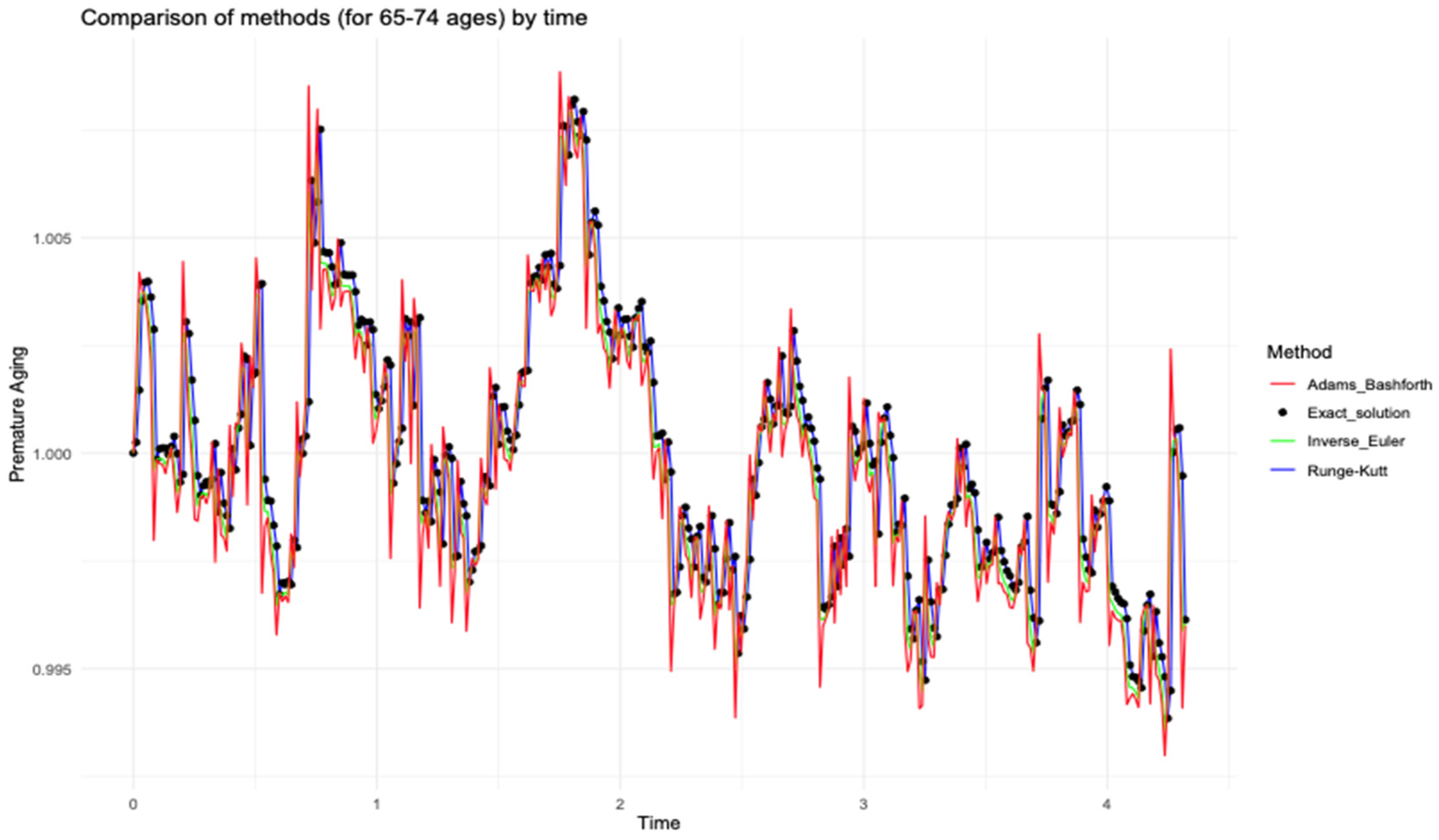
The results obtained through various mathematical modeling approaches are visually presented in the following figures. Figure 5, Figure 6 and Figure 7 demonstrate the behaviors of premature aging change over time t for different age categories with the proposed methods.

Figure 5, Figure 6 and Figure 7 demonstrate a strong agreement between the numerical modeling results for all categories using the fourth-order Runge–Kutta method and the exact (analytical) solution. This consistency helped optimize the process of selecting the most suitable method for further analysis.

According to the Table 1 and Figure 5, Figure 6 and Figure 7, we can see that correlation coefficients in different age groups differed: in the 65–74 category, they were higher, in the 74–89 and 90+ categories, coefficients were significantly lower. These differences may indicate different rates of ageing processes depending on age.

Thus, the analysis conducted using various methodologies provided a comprehensive understanding of age-related changes in the cardiovascular system. The selected biomarkers formed interactions that reflected the degree of influence of various factors on the aging processes in each age category. In the 65–74-year-old group, the correlation coefficients were the highest, which may indicate a more pronounced influence of biomarkers on age-related changes. In the 75–89-year-old category, the values of the coefficients decreased, and in the 90+-year-old group, they became even more balanced, which may indicate that the correlations between biomarkers decrease with age.

This implies that in the early stages of aging, the influence of biomarkers is more pronounced, whereas at later ages, other factors such as accumulated age-related changes, chronic diseases, or adaptive mechanisms may reduce the importance of individual biomarkers in modelling the rate of aging.

Differences between the numerical and exact solutions were found (see

Table 3. Values of accuracy orders of numerical methods.

Solution Methods	Order of Method	Age Category	Maximum Error with Exact Solution
Runge–Kutta	$O\left({∆x}^4\right)$	65–74	0.00002677413
		75–89	0.0004091325
		90+	0.00004571414
Adams–Bashforth	$O\left({∆x}^2\right)$	65–74	0.007965958
		75–89	0.03635441
		90+	0.01277912
Backward Euler	$O\left(∆x\right)$	65–74	0.005310639
		75–89	0.02423627
		90+	0.008519411

).

Comparison of the maximum error of the selected numerical methods with the exact solution for each age group is presented in Table 3. The Runge-Kutta method demonstrated the highest order of accuracy among the methods considered. Maximum errors of $max\left|x_i^{exact}-x_i^{Runge-Kutt}\right|=0.00002677413$, $max\left|x_i^{exact}-x_i^{Runge-Kutt}\right|=0.0004091325$, and $max\left|x_i^{exact}-x_i^{Runge-Kutt}\right|=0.00004571414$ were found for the age groups 65–74, 75–89, and 90+, respectively. These values were the smallest among all methods, which indicated the high accuracy of the numerical solution. The Runge–Kutta method provided the best agreement with the analytical (exact) solution.

The Adams–Bashforth method had a lower order of accuracy compared to the Runge–Kutta method. Its maximum errors were $max\left|x_i^{exact}-x_i^{Adams-Bashforth}\right|=0.007965958$, $max\left|x_i^{exact}-x_i^{Adams-Bashforth}\right|=0.03635441$, $max\left|x_i^{exact}-x_i^{Adams-Bashforth}\right|=0.01277912$ for the age categories 65–74, 75–89, and 90+, respectively, significantly higher, especially in the 75–89 age category, indicating a lower accuracy of the method.

The backward Euler method had the lowest orders of accuracy $max\left|x_i^{exact}-x_i^{BackwardEuler}\right|=0.005310639$, $max\left|x_i^{exact}-x_i^{BackwardEuler}\right|=0.02423627$, and $max\left|x_i^{exact}-x_i^{BackwardEuler}\right|=0.008519411$ for the age groups 65–74, 75–89, and 90+, respectively. Although this method has a simple implementation, its high uncertainty makes it less favorable for our application, especially in age groups with large data variation.

Based on the obtained data, the fourth-order Runge–Kutta method (O(∆x⁴)) was the optimal choice for the numerical solution of the considered problem, as it improved the accuracy of the numerical solution by providing the smallest errors and the best agreement with the analytical calculations.

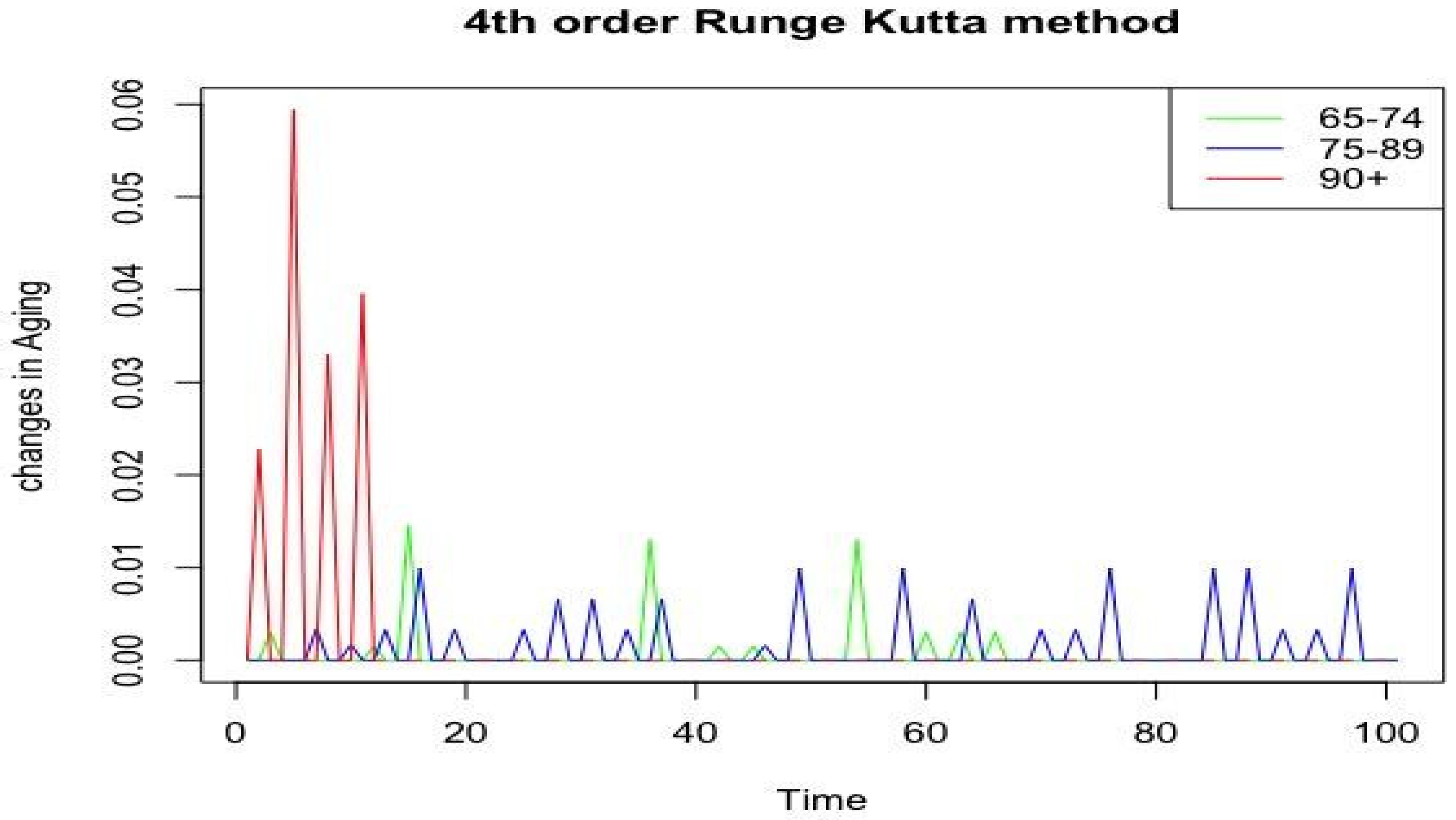
Next, let us consider our problem using the already selected fourth-order Runge–Kutta method. Figure 8 presents data illustrating changes in the ageing process for the three age groups: 65–74 years old, 75–89 years old, and 90+ years old. The abscissa axis (horizontal axis) denotes time, and the ordinate axis (vertical axis) shows the changes in aging according to Figure 2, Figure 3 and Figure 4.

In the 65–74 age group, moderate fluctuations in indicators with relatively low amplitude were observed, which may indicate a more stable aging process in that interval. In that group, the influence of bad habits, such as alcohol consumption and smoking, on the development of postinfarction cardiosclerosis (correlation coefficient b₁), increased blood pressure, as well as changes in body weight, which may accelerate the aging process, was noted.

In the 75–89 age category, the amplitude of the fluctuations was higher than in 65–74-year-olds but lower than in persons over 90 years of age, indicating the intermediate nature of changes associated with aging. For that group, we can assume that the aging process is associated with the level of a₂ interaction with the increase in blood pressure, the appearance of the c₂ correlation coefficient reflecting the risk of developing chronic heart failure, as well as the d₂ coefficient characterizing the probability of coronary heart disease.

The analysis of the graphs showed that the peaks in each age category may correspond to the time intervals during which the ageing processes were most intensive.

The group of 65–74-year-olds showed the most stable dynamics of changes, probably due to the influence of bad habits, which may indicate a more predictable nature of ageing at that age. On the contrary, the group of 90+-year-olds showed the greatest fluctuations, which may indicate a decrease in the predictability of the ageing process or its increased sensitivity to various factors, such as the respondent’s gender, level of education, and smoking.

Thus, with the numerical implementation of the model using the Runge–Kutta, Adams–Bashforth, and backward Euler methods, we observed a high degree of consistency between the approximate and exact solutions. This agreement confirmed both the mathematical validity and computational stability of the proposed differential equation system.

Building upon this foundation of numerical reliability, the second phase of the study focused on enhancing predictive capabilities through machine learning. While the initial stage of the study was focused on numerical modeling of cardiovascular risk factors, we further conducted an external validation using a Random Forest classifier to test the generalizability of the model. The model, trained on the 65–74 cohort, was applied to independent subgroups (75–89 and 90+ years) using the same features.

Results showed that the model maintained high predictive accuracy without recalibration, achieving AUC = 0.989 in the 75–89 group and 1.000 in the 90+ group, indicating strong extrapolation across age categories.

The validation results demonstrated high predictive performance across key evaluation metrics (Table 3).

The model achieved an overall accuracy of 98.8% (see

Table 4. External validation results.

Metric	Value
Accuracy	98.8%
F1-score (class 0)	0.98
F1-score (class 1)	0.99
ROC AUC	0.989

), indicating a high proportion of correct predictions across both classes. The F1-scores of 0.98 for class 0 (absence of condition) and 0.99 for class 1 (presence of condition) reflected strong precision–recall balance and robustness across class distributions.

Furthermore, the area under the ROC curve (AUC) was 0.989, demonstrating excellent discrimination between patients with and without the target condition (e.g., ischemic heart disease). These results confirmed that the model retained its predictive capability when applied to an independent population of older individuals.

These results support the conclusion that the developed ODE-based mathematical model, when solved using standard numerical methods and trained on representative clinical data, can accurately predict cardiovascular aging trajectories across elderly subpopulations. The consistency of performance across age groups reinforces the model’s potential for application in real-world preventive cardiology and geriatric risk stratification.

Having validated the model using numerical methods and supervised machine learning approaches, we then proceeded to explore the potential of unsupervised learning for pattern discovery in the data.

To complement the supervised analysis, a clustering model based on the k-means algorithm (k-means) was developed and tested for automatic segmentation of clinical data from patients with suspected cardiovascular disease (CVD). The main objective was to test the hypothesis that without predefined labels, the model based on unsupervised learning could categorize patients into groups with different cardiovascular status—with and without CVD.

Despite the presence of classes in the original medical records, they were not included in the model, as the task was specifically to independently identify the structure of the data using the k-means algorithm.

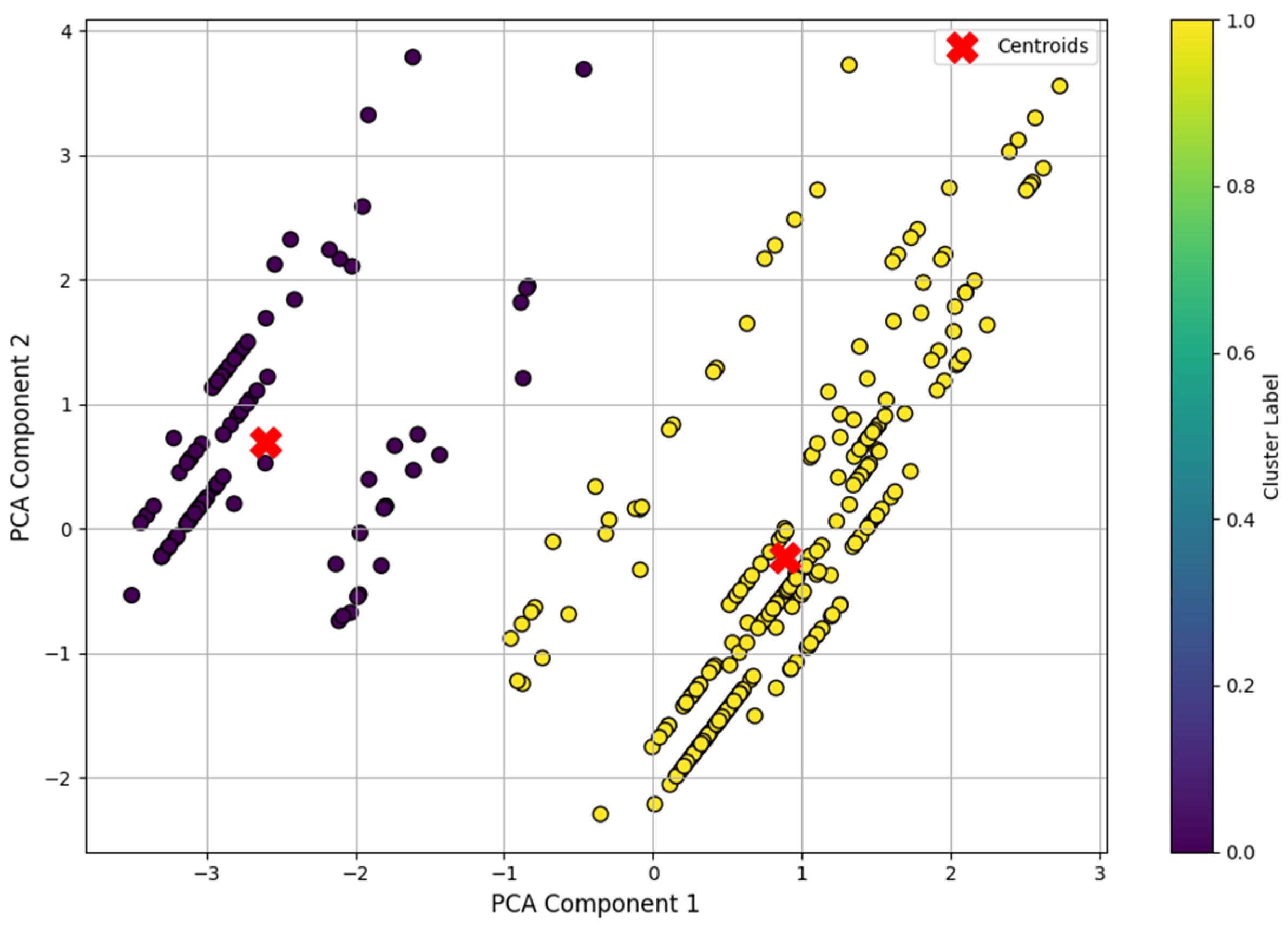
To ensure robustness of the results and clarity of visualization, the data were first normalized using standardization and then transformed into a two-dimensional space using the principal component analysis (PCA) method.

After applying the principal component method (PCA), two-dimensional projections of the training data were visualized on a plane, where color differentiation marked the membership of objects to the corresponding clusters identified by the k-means algorithm. The coordinates of the centroids of the clusters were also marked on the plot, which allowed us to analyze the spatial distribution of the groups (Figure 9). The observed clear separation into two distinct areas confirmed the correct segmentation of the sample and demonstrated the ability of the model to identify the internal structure of the data without using class labels.

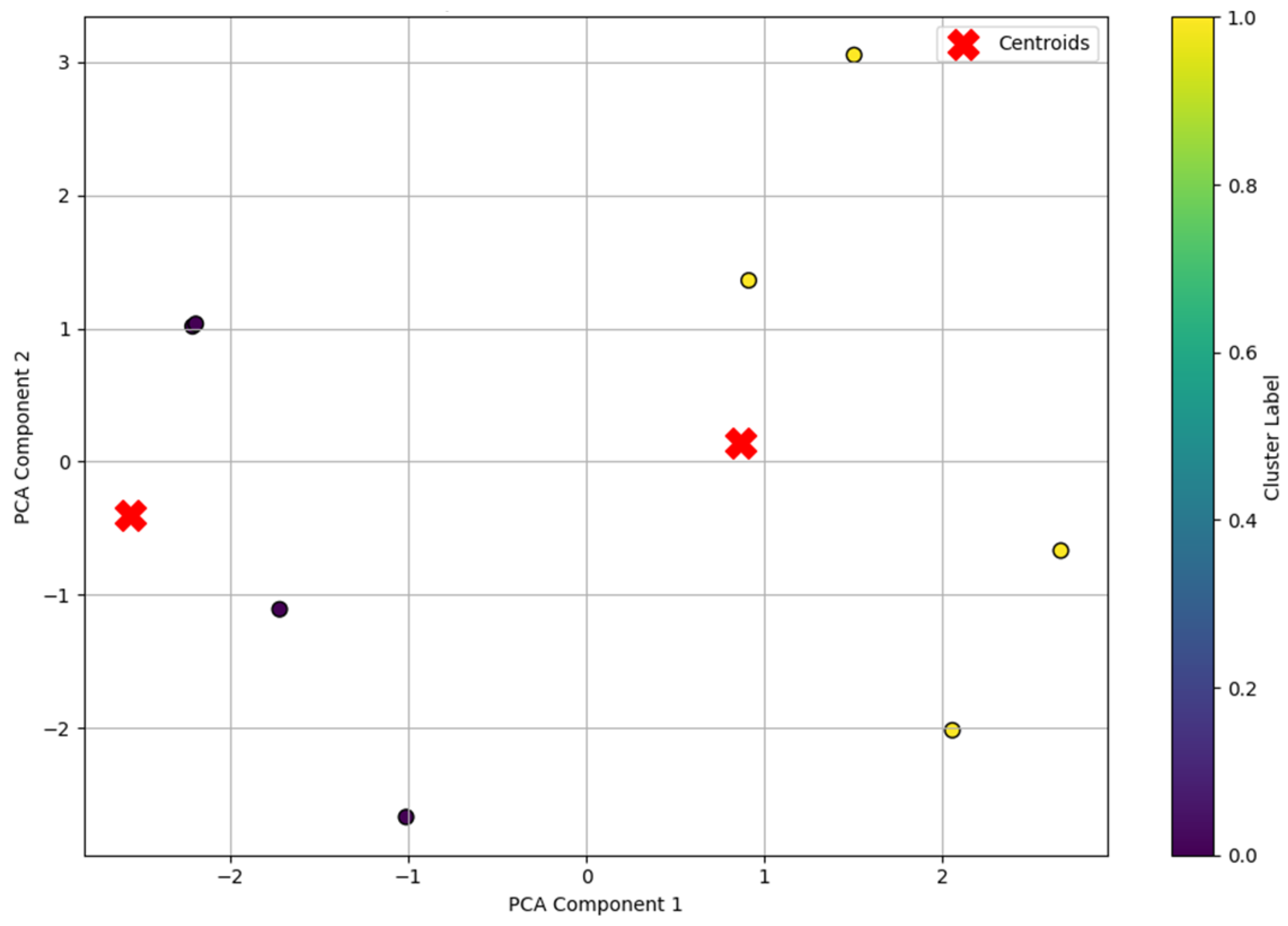
Similar visualization was performed for the independent test dataset (df1), which was not used in the model training phase. The first four observations corresponded to patients without cardiovascular disease (class 0), while the last four patients belonged to the group with an established diagnosis of CVD (class 1). However, this information was deliberately not provided to the model during the prediction phase, as the aim of the study was to test the ability of the clustering algorithm to independently identify this separation solely based on internal patterns in the original features. This dataset was processed using the same normalization methods and projection into PCA space, after which cluster labels were predicted using the pre-trained k-means model.

The resulting visual pattern (Figure 10) showed a stable and homogeneous clustering like the training sample, indicating the high robustness of the model and its ability to generalize to new data. The “Cluster Label” color scale in the graph indicates the belonging of each point to one of the two clusters extracted by the k-means algorithm, where zero and one are the numbers of the corresponding clusters.

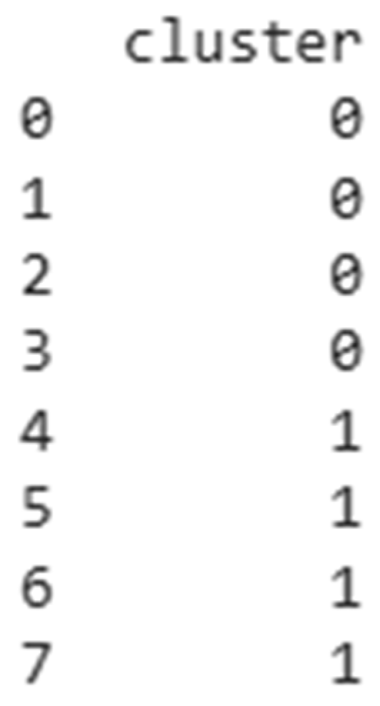
Despite the fact that the model did not use class labels, it was known that the test sample df1 contained a hidden (implicit) structure corresponding to the true distribution of patients according to the presence of CVD. A comparison of the predicted clusters with the known but hidden information showed complete correspondence (Figure 11)—all patients were correctly assigned to the corresponding groups. This allowed the external validation of the clustering results, confirming the high accuracy and significance of the extracted features.

Therefore, the analysis showed that the developed clustering model based on the k-means algorithm was highly effective when working with clinical data that did not contain explicit class labels. The model successfully identified the latent structure in medical indicators and demonstrated the ability to detect latent patterns specific to different patient groups. The external validation performed on an independent dataset showed the full agreement of the clustering results with the actual distribution of patients by cardiovascular health status, which confirmed the high accuracy of the model. Taking this into account, the proposed approach can be recommended for use in primary screening and preliminary patient segmentation tasks, especially in cases when the data do not contain annotated classes or are at the stage of primary analysis.

The model has a number of limitations. It depends on the quality and completeness of clinical data, which may affect its generalizability. The selected biomarkers represent only part of the complex aging process. The model was trained on a specific cohort; therefore, further testing on broader populations is needed.

4. Conclusions

In conclusion, the proposed mathematical model demonstrated a high level of consistency and accuracy when solving cardiovascular aging dynamics using numerical methods such as Runge–Kutta, Adams–Bashforth, and backward Euler. The close match between numerical and exact solutions confirmed the correctness and stability of the model. The originality and scientific significance of this model were supported by its registration in the State Copyright Register (No. 46336, dated 23 May 2024).

To evaluate its real-world applicability, we performed external validation using clinical data from elderly patients. The model was trained and tested on older age groups using a Random Forest classifier. The results showed high predictive performance, with an accuracy of 98.8% and an AUC of 0.989.

In addition, we applied k-means clustering to identify subgroups of patients with similar clinical profiles. This allowed us to uncover meaningful patterns in the data and better understand the distribution of cardiovascular risk across different patient clusters.

Thus, risk modelling showed that in the elderly, behavioral, and metabolic factors significantly influenced cardiovascular health. In 65–74-year-olds, smoking and alcohol increased the risk of infarction and hypertension by up to 53%, in the 75–89-year-old group, the risk of hypertension and CVD by up to 21%, and in the 90+ age group, hypercholesterolemia increased the risk of CVD by 17%. These data confirmed the importance of an age-specific approach to the prevention of cardiovascular ageing.

Overall, the integration of mathematical modeling, machine learning classification, and unsupervised clustering provides a comprehensive framework for predicting cardiovascular aging. The model may serve as a valuable tool in geriatric healthcare for developing personalized prevention strategies and improving the quality of life in the elderly population.