1. Introduction
The rise in e-commerce has fundamentally changed consumer shopping habits. Nowadays, consumers have quick access to a vast array of alternatives and offers through electronic devices, which has fueled the rapid growth of e-commerce and led to a significant increase in the demand for parcel delivery [
1]. The ability of logistics companies to efficiently deliver parcels to customers is one of the key factors in the success of e-commerce. With the surge in demand for parcel delivery, the logistics industry is booming. However, in an intensely competitive market, cost reduction as the only goal is no longer sufficient to enhance the market competitiveness of logistics companies. How to cope with customers’ increasing demands for service quality has become the key to enhance the market competitiveness of enterprises [
2]. In logistics delivery, the last mile of delivery is directly facing the customers [
3], which is the key link to improve the service quality. In this process, customer satisfaction, as an important indicator for measuring the service quality of logistics companies, has received widespread attention.
In last-mile delivery, customer satisfaction is usually assessed by the timeliness of delivery [
4]. Researchers have proposed a variety of descriptions related to delivery time, such as customer waiting time cumulative function [
5] and fuzzy time window function [
6]. However, customer satisfaction is a subjective metric that is influenced by customers’ psychological behavior. The above methods cannot adequately capture customers’ psychological behaviors, so the obtained customer satisfaction often deviates from the actual situation [
7,
8,
9]. For this reason, this paper improves the traditional way of describing customer satisfaction based on prospect theory. Specifically, when considering the customer’s psychological reference point in delivery time, the customer’s expectations are met when the delivery vehicle arrives early or on time; while when the vehicle is late, the customer’s satisfaction will show a different response based on the customer’s psychological behavior. This update better reflects customers’ psychological responses in different delivery scenarios, thus providing a more realistic evaluation of customer satisfaction.
In addition, due to the division of urban areas (e.g., work, living, and recreational areas) and the differences in the living habits of customers, logistics companies often have to make secondary deliveries due to the absence of the customer when designating the delivery location [
10], which leads to a reduction in the efficiency of delivery. Obviously, this not only has a negative impact on transport cost but is also detrimental to the achievement of ecological goals. Current delivery models usually allow customers to choose only one delivery location; however, since the customer’s activity location is not fixed, this can easily lead to a mismatch between the customer’s actual activity location and the selected delivery location. To address this problem, this paper proposes a new delivery model that allows customers to provide flexible optional delivery locations in a single delivery service, thereby improving delivery flexibility. This improvement is expected to reduce the occurrence of secondary deliveries and enhance logistics efficiency while reducing transport costs and environmental impact.
Vehicle Routing Problems (VRPs) represent a core challenge in logistics and operations research, focusing on optimizing delivery routes to minimize costs while meeting various constraints. In today’s competitive landscape, particularly in e-commerce driven last-mile delivery, ensuring high levels of customer satisfaction has become as critical as cost efficiency.
Therefore, with the goal of completing the delivery service at the right place at the right time, this paper explores how to describe customers’ psychological expectations of delivery time through a customer satisfaction function and solve the vehicle routing problem of last-mile delivery considering customer satisfaction.
Although significant progress has been made in VRP research, existing studies still fall short in addressing problems with flexible delivery options and in analyzing the impact of customer behavioral psychology on satisfaction. Most existing VRP models tend to oversimplify satisfaction measurement or focus solely on delivery flexibility, lacking a comprehensive consideration of both aspects. This study addresses this gap by proposing the VRP-CS, which incorporates a customer satisfaction evaluation method based on prospect theory, analyzing preferences from the perspectives of both delivery time and delivery location.
The introduction of flexible delivery options and the incorporation of a satisfaction model significantly increase the complexity of the problem, posing challenges to traditional solution methods. To efficiently tackle this bi-objective and computationally demanding problem, the MSALNS algorithm is developed. The proposed algorithm introduces neighborhood operators based on customer satisfaction, which expand the search space of the algorithm and improve the convergence speed. In addition, an adaptive mechanism that dynamically adjusts search strategies based on real-time feedback from the search process is designed, which solves the problem of ALNS easily falling into local optima and improves the solution quality. These enhancements not only improve the solution quality but also ensure faster convergence and robust performance across diverse problem instances.
The main contributions of this paper are as follows:
A Vehicle Routing Problem with flexible delivery time and locations is proposed, which considers customers’ preferences for different delivery times and locations.
A satisfaction evaluation method based on prospect theory is introduced, which incorporates customers’ loss aversion and evaluates satisfaction from two aspects: delivery location and delivery time.
A MSALNS algorithm is proposed. In the search phase, neighborhood structures guided by strategies such as backtracking are designed to expand the search space and accelerate convergence. In the adaptive phase, a simulated annealing-inspired acceptance criterion is adopted to prevent premature convergence to local optima and to enhance solution quality.
The rest of the paper is organized as follows:
Section 2 reviews related literature;
Section 3 describes the problem and formulates a MINP model of the proposed problem;
Section 4 presents the details of the MSALNS;
Section 5 designs numerical experiments to evaluate the proposed model and algorithm; and
Section 6 provides concluding remarks and pointers for further research.
2. Literature Review
The vehicle routing problem (VRP) was originally proposed by Dantzig and Ramser [
11] and applied in logistics and distribution. Many scholars have studied it thereafter [
12,
13,
14,
15].
This section summarizes and analyses the vehicle routing problem from two perspectives: the vehicle routing problem considering customer satisfaction (VRP-CS) and the vehicle routing problem with delivery options (VRPDO). The VRP-CS proposed in this paper is a variant of the VRPDO in which each customer has multiple time-dependent locations and in which customer satisfaction is considered.
2.1. The Vehicle Routing Problem Considering Customer Satisfaction
Nowadays, e-commerce platforms in the market have established an online delivery service evaluation system, which prompts logistics providers to pay attention to customer satisfaction and take improving customer satisfaction as a major key to improving their competitiveness. Therefore, the study of customer satisfaction has also become an important research direction for related researchers and practitioners in the field of logistics service supply chain. In the research field of the VRP, some scholars have conducted research on customer satisfaction. Unlike delivery time, customer satisfaction is an abstract concept, and scholars have proposed different approaches to analyze customer satisfaction.
Early studies mainly associated customer satisfaction with delivery punctuality. Fan [
16] considers customer satisfaction in a VRP with simultaneous pickup and delivery; they argue that customer satisfaction is inversely proportional to the amount of time the customer waits for the vehicle, that each delivery has to be met as early as possible, and that their problem aims to improve total customer satisfaction. Qin et al. [
17] use delivery punctuality as an evaluation criterion for customer satisfaction: when the delivery occurs within the time window, the customer feels fully satisfied; otherwise, the customer will feel dissatisfied. In their study, they use average satisfaction as the target, which effectively improves the average customer satisfaction by a small increase in the cost.
To better capture subjective perceptions, some scholars introduced piecewise functions to model customer satisfaction. Afshar-Bakeshloo et al. [
18] propose a segmented linear fuzzy time window service level function by using a combination of soft- and hard-time windows combined with delivery time to explain subjective customer satisfaction. Yu et al. [
19] aimed to ensure customer satisfaction by improving time consistency and driver consistency, while also taking driver fairness into account. They proposed an adaptive large neighborhood search algorithm to address this problem, effectively ensuring consistency in drivers’ travel distances. Su et al. [
20], on the other hand, proposed a segmented linear function incorporating a time window to assess customer satisfaction. For customers who complete the delivery before the time window, they show complete satisfaction; for customers who complete the delivery after the time window, their satisfaction is minimized. Within the time window, satisfaction decreases linearly as delivery is delayed. In this way, customer satisfaction can be assessed based on the specific time when delivery occurs. Yue et al. [
21] proposed a segmented rating method for assessing customer satisfaction. Completion of deliveries in different time windows produces different satisfaction ratings, which are used as an evaluation metric for customer satisfaction. Xu et al. [
22] considered dual aspects of customer satisfaction in community group buying, including time satisfaction and freshness satisfaction. They used a piecewise function to evaluate customer satisfaction corresponding to different service times.
However, these piecewise linear models often oversimplify customer psychology. Stavropoulou [
23] considers customer satisfaction in a consistent vehicle routing problem with heterogeneous fleet, and they use the consistency of the service and the consistency of the delivery time as the target as a way of improving overall customer satisfaction to ensure customer retention and brand loyalty. Cui et al. [
24] investigated the impact of delivery timeliness on customer satisfaction and observed that customer satisfaction exhibits different trends when delivery occurs in the early versus the late stages of the customer’s time window. Zheng et al. [
25] categorized customers based on their delivery time preferences and proposed a fuzzy clustering optimization approach to guide logistics enterprises in effective distribution management. Wang et al. [
26] studied customer satisfaction under time-varying speeds by simulating urban traffic flow variations, effectively analyzing the relationship between vehicle speed and customer satisfaction. These studies suggest that the relationship between delivery time and customer satisfaction is not purely linear and requires a more nuanced modeling approach.
In response, recent research has begun to adopt behavioral economic theories to better describe satisfaction dynamics. Huang et al. [
27] evaluated customer satisfaction by considering delivery time in fresh urban logistics distribution. They used prospect theory to analyze customer psychological behavior considering delivery time and constructed corresponding time satisfaction function, effectively ensuring customer experience in delivery services.
In summary, the existing literature highlights the importance of modeling customer satisfaction based on delivery time in VRP. Piecewise functions are widely used to describe satisfaction variations across different time intervals, reflecting that customers may respond differently to deliveries occurring early, on time, or late. However, these approaches often rely on linear or piecewise linear functions, which may fail to capture the asymmetric psychological effects associated with early versus late deliveries. This limitation is addressed in our work by incorporating prospect theory, which enables a more realistic and behaviorally grounded modeling of customer satisfaction. By reflecting loss aversion and other psychological characteristics, the proposed model supports more accurate and customer-centric delivery optimization in last-mile logistics.
2.2. The Vehicle Routing Problem with Delivery Options
The integration of delivery options into vehicle routing problems (VRPs) introduces flexibility by allowing deliveries to the same customer to occur at different locations, each associated with distinct time windows. This feature is particularly relevant in last-mile logistics, where customer behavior and urban constraints demand adaptable delivery strategies.
Reyes et al. [
28] proposed a VRP with roaming delivery locations (VRPRDL), where the logistics provider chooses a location among several delivery options based on a schedule and delivers the goods to the trunk of the customer’s car. This problem is solved using Large Neighborhood Search (LNS) heuristic algorithms and experimentally analyzed; the roaming delivery approach leads to significant economic and environmental benefits. It needs to be noted that they assumed that the customer does not move faster than the delivery vehicle, which helps them to propose a strategy to speed up the algorithm while also limiting the applicability of the problem. Ozbaygin et al. [
29] modeled the VRPRDL problem as a set covering the problem and developing a branch-and-price (B&P) algorithm to solve the problem with an average savings of 20% on the experimental dataset, a solution not suitable for large-scale problems. Dumez et al. [
30] additionally allowed customers to specify preferred delivery locations in addition to considering delivery options, and finally solved this problem using a large neighborhood search algorithm, obtaining good results on both small and large problems, finally providing some management insights for the vehicle routing problem with delivery options.
Several studies further explored delivery flexibility through customer-defined delivery preferences. Ransikarbum et al. [
31] applied the k-means clustering algorithm to evaluate potential locations for raw material collection points in the upstream supply chain. They formulated the problem as a vehicle routing problem with flexible time windows, aiming to minimize the total delivery cost while ensuring low delivery delays. Voigt et al. [
32] allowed each customer to be associated with a set of delivery time windows in order to reflect the implicit requirement for customer presence in real-world delivery scenarios. They proposed a hybrid ALNS algorithm to solve this problem, which effectively reduced delivery costs while minimizing failed deliveries. Schaap et al. [
33] observed that narrower time windows can enhance customer satisfaction but may restrict the delivery flexibility of logistics companies. To address this, they studied how to select the optimal time window for each customer from multiple available options, aiming to balance customer satisfaction and delivery cost. They proposed an improved large neighborhood search algorithm to solve this problem, and the results showed that offering multiple time windows can bring economic benefits to logistics providers. Chen et al. [
34] formulated a three-dimensional vehicle routing problem in last-mile delivery by incorporating vertical travel time, hard time window constraints, and delivery options, and proposed a crowding differential evolution algorithm to minimize cost while enhancing customer satisfaction.
Other scholars introduced delivery option flexibility in various forms. Karimi et al. [
35] considered customers’ preferences for delivery locations and formulated a two-echelon vehicle routing problem, effectively balancing delivery costs with customer preferences. Zhang et al. [
36] addressed the problem of simultaneous pickup and delivery by offering customers the option to choose self-pickup locations along with compensation incentives. They developed a customized adaptive large neighborhood search algorithm to effectively solve the problem. The results showed that this approach significantly reduced delivery costs. Niu et al. [
3] allowed consumers to provide multiple delivery locations as well as corresponding time window constraints in urban logistics and distribution using a delivery model with delivery options. They solved this problem by using a large neighborhood search algorithm to improve the probability of consumers receiving the goods in time. Frey et al. [
37] proposed a vehicle routing problem with time windows and flexible delivery locations. They set the capacity of different service locations based on a real-time therapist scheduling problem. To solve this problem, they developed a hybrid adaptive large neighborhood search algorithm and analyzed it experimentally on real hospital data, which greatly improved the quality of the solution. Zhao et al. [
2] proposed a vehicle routing problem that considers customer preferences for delivery options. They used a probabilistic model to represent the degree of customer preference for deliveries to different locations and different time windows by analyzing customer data and further used an ALNS approach to solve the problem.
Collectively, these studies highlight how delivery options enhance VRP flexibility, enabling logistics providers to reduce operational costs while improving customer satisfaction. However, many of these works focus primarily on cost efficiency and operational feasibility, often treating customer satisfaction as a secondary or implicit outcome.
Given the proven effectiveness of ALNS in handling complex VRP variants with time window constraints and delivery flexibility, we adopt an MSALNS algorithm in this work. This allows us to better capture customer satisfaction as a primary optimization objective while maintaining high-quality solutions for cost and efficiency. The MSALSN builds on the ALNS framework by incorporating customer satisfaction into the design of neighborhood structures, which expands the search space and accelerates convergence. In addition, a multi-annealing mechanism is used to prevent the algorithm from getting stuck in local optima too early, thus improving solution quality [
38,
39].
3. Problem Description and Formulation of the VRP-CS
This section details the formal description and mathematical formulation of the proposed Vehicle Routing Problem considering Customer Satisfaction (VRP-CS). The formulation itself, integrating flexible delivery options with prospect theory-based satisfaction, represents a key theoretical contribution of this work.
Section 3.1 provides a formal problem description.
Section 3.2 outlines the necessary assumptions for the model and introduces the corresponding notation.
Section 3.3 presents the mixed nonlinear integer problem formulation of the VRP-CS problem and discusses the corresponding linearization.
Section 3.4 introduces the customer satisfaction function.
3.1. Problem Description
The VRP-CS addressed in this paper seeks to optimize last-mile delivery operations by designing efficient vehicle routes while maximizing customer satisfaction. Formally, the problem can be defined as follows: Given a central depot, a fleet of homogeneous vehicles with limited capacity, and a set of customers each with specific demands and multiple potential delivery locations (each associated with a time window and influencing customer satisfaction based on arrival time), the objective is to determine a set of minimum cost vehicle routes originating and terminating at the depot such that all customer demands are met exactly once at one of their specified locations within its time window, vehicle capacities are not exceeded, route constraints are respected, and overall customer satisfaction (modeled using prospect theory) is maximized alongside cost minimization.
The specific components of the problem are detailed below:
Depot: There is a single central depot (indexed as ) from which all deliveries originate and where all vehicles must return after completing their routes. The depot has a specific operating time window, , defining the earliest departure time () and the latest allowed return time () for all vehicles.
Vehicles: A fleet of homogeneous vehicles is available at the depot. Each vehicle has an identical maximum load capacity and operates at the same average travel speed . A fixed operating cost may be associated with using each vehicle.
Customers and Demands: A set of customers requires delivery service. Each customer has a known demand , which must be fully satisfied by a single delivery (split deliveries are not allowed). The demand of each customer is assumed to be less than the vehicle capacity ().
Delivery Options and Time Windows: A key feature of the VRP-CS is delivery flexibility. Each customer
provides a set
of acceptable optional delivery locations. For each potential delivery location
, there is a specific time window
during which the delivery must be started. If a vehicle arrives at a location before the earliest time
, it must wait until
to begin service. Service at each location takes a constant time
. The selection of a specific location
and the timing of the service within
influences the route planning and customer satisfaction.
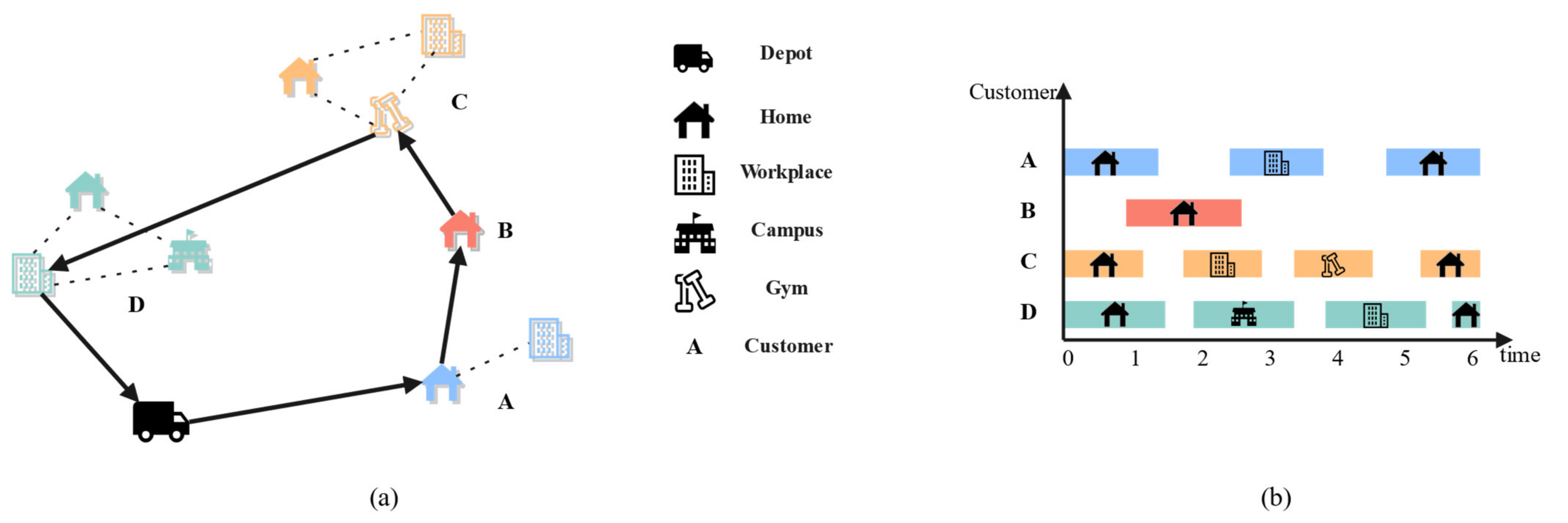
Figure 1 illustrates this concept of multiple locations per customer itinerary.
Costs: The primary cost objective is to minimize the total operational cost. This includes the total distance traveled by all vehicles, calculated based on the distances between the chosen delivery location for customer and location for customer (or the depot). Additionally, there is a cost component associated with deviations from desired customer satisfaction levels, integrated into the objective function.
Satisfaction Objective: Distinct from traditional VRPs, the VRP-CS explicitly incorporates customer satisfaction as a second, conflicting objective to be optimized (maximized). Customer satisfaction
for customer
at location
is modeled as a nonlinear function based on prospect theory. It depends crucially on the actual service start time
relative to the customer’s psychological reference point
for that location, capturing the asymmetric perception of gains (early/on-time arrival) versus losses (late arrival). The formal definition of this satisfaction function is provided in
Section 3.4.
The VRP-CS aims to find feasible routes and select one delivery option (location and associated time) for each customer to minimize the combined costs related to travel, vehicle usage, and customer dissatisfaction.
As shown in
Figure 1, each customer has their own itinerary. This itinerary represents optional delivery options and their time windows. It specifies when and where the customer’s order can be delivered.
3.2. Assumptions and Decision Variables
3.2.1. Model Assumptions
The complex factors in logistics distribution increase the difficulty of solving the VRP-CS, some of which are not necessary to achieve the core optimization goal. By putting forward reasonable assumptions, the problem can be simplified, and the solvability of the model can be improved. Therefore, the VRP-CS makes the following assumptions:
The logistics supplier has enough vehicles at the distribution center to complete the delivery task.
Each customer can only be served in one time window at one location, and the service must be completed within the time window at that location. A vehicle can only be used to serve a customer once.
All customer services must be completed within the specified scheduled time window.
Split delivery is not permitted, and the requirements of every single customer do not exceed the maximum load of a single vehicle.
3.2.2. Decision Variables
The VRP-CS model utilizes the following decision variables to determine the optimal routing plan and delivery assignments:
: This is a binary variable indicating the sequence of deliveries. It equals 1 if vehicle travels directly from location (an optional delivery location for customer or the depot if ) to location (an optional delivery location for customer or the depot if ), and 0 otherwise. This variable defines the specific arcs traversed by each vehicle in the solution routes.
: This is a binary variable representing the assignment of customers to vehicles and specific delivery locations. It equals 1 if customer ’s optional delivery location is selected and served by vehicle , and 0 otherwise. This ensures each customer is served exactly once at one chosen location by one vehicle.
: This continuous variable represents the time at which service begins for customer at their chosen optional delivery location . This variable is crucial for checking time window feasibility and calculating customer satisfaction.
: This continuous variable represents the calculated customer satisfaction level for customer
when served at optional location
. Its value is derived from the arrival time
relative to the customer’s expectations using the satisfaction function defined in
Section 3.4, ranging between −1 (maximum dissatisfaction) and 1 (maximum satisfaction).
: This is a binary variable indicating whether vehicle is used in the delivery plan. It equals 1 if vehicle serves at least one customer and 0 otherwise. This variable is used to account for fixed vehicle usage costs.
Table A1 and
Table A2 summarize all the symbols used in the mathematical model for the above problem.
3.3. Objective Function Mathematical Formulation
Based on the above scenario description and assumptions, the following mathematical model for the VRP-CS is established through the analysis of the problem model:
In the formulations above, the objective function (1) aims to minimize the total distribution cost. Constraint (2) states that each customer is served only once at one of the optional locations. Constraint (3) states that a customer can only be served by a vehicle at one of the optional locations. Constraint (4) indicates that the service occurs at a location that is passed by a vehicle. Constraint (5) is the flow conservation constraint, which states that a vehicle must leave after serving a customer. Constraint (6) states that a vehicle must start and end its journey at the depot. Constraint (7) states the relationship between the start times of the visits to the adjacent customer points. Constraint (8) states that the vehicle serves the customer strictly within the requested time window. Constraint (9) states that the load of the vehicle cannot exceed its capacity. Constraint (10) represents the constraint on the distance traveled by the vehicles, which cannot exceed a maximum distance. Constraint (11) represents whether the vehicle is in use. Constraints (12) and (13) define the binary variables and .
3.4. Customer Satisfaction Function
In the VRP-CS, the optional delivery locations and variable delivery time are effective means to improve customer satisfaction. Customer satisfaction is influenced by the psychological factors of customers, who are more sensitive to poor delivery services. This trend can be well assessed using the loss aversion concept of prospect theory.
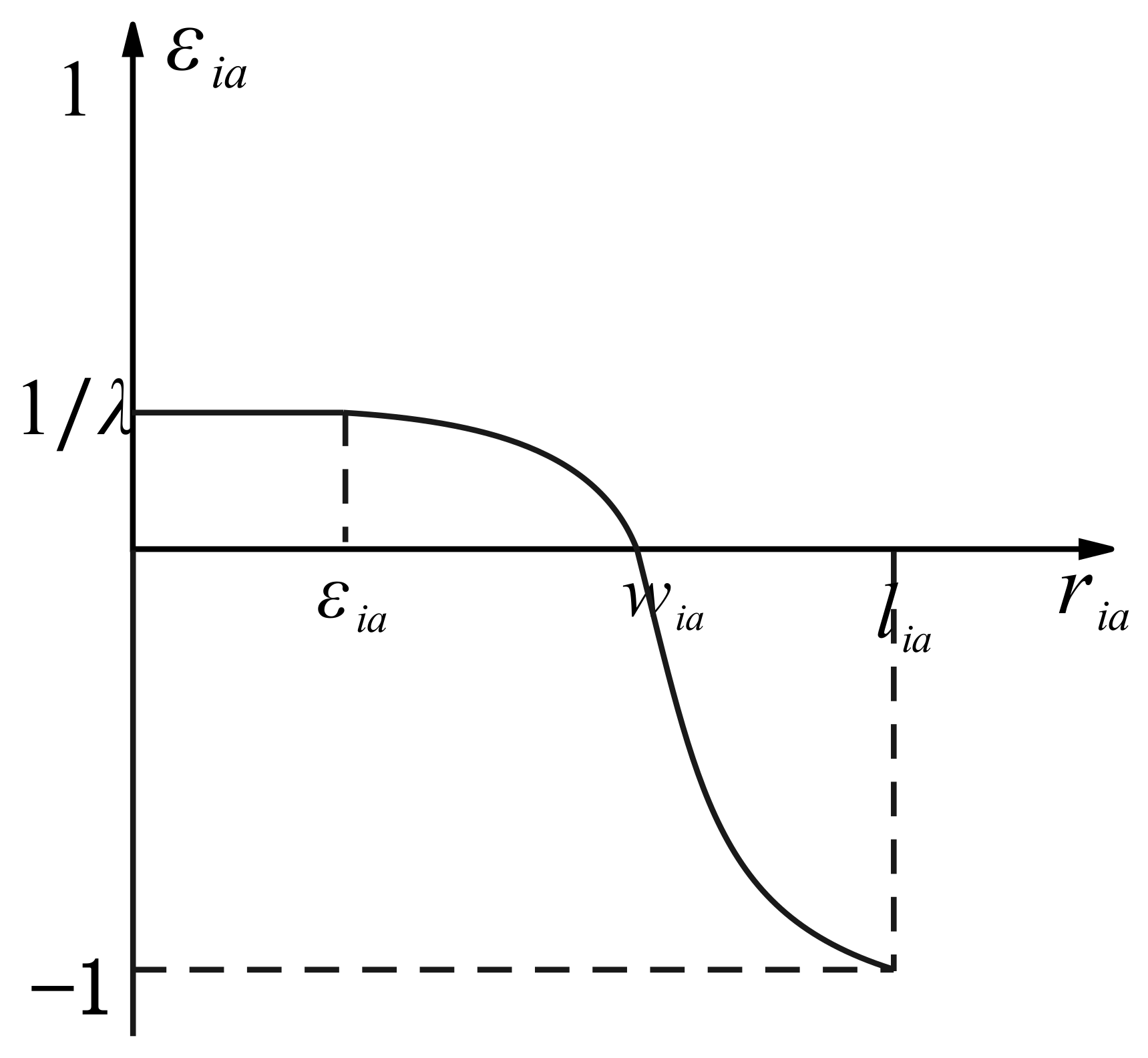
Therefore, a nonlinear satisfaction change curve based on prospect theory is provided. For deliveries that are later than the psychological reference point, a penalty is applied (i.e., the satisfaction value is negative). Conversely, when the vehicle arrives early, a reward is given (i.e., the satisfaction value is positive). Combining the above research, the customer satisfaction function is defined as follows:
The
represents the satisfaction benefit obtained by customer
when receiving delivery at location
calculated using formula (14), with a value range of (−1,1), and the value of
for unused location is 0. The moment when the customer receives the service is represented by
, the customer’s psychological reference point for receiving service at location
is
, we use
to represent the time window width of this location,
represents the time span from a to b,
and
are the risk attitude coefficients, which usually take on values between 0 and 1. The larger the value, the more likely the individual is to take risks.
represents the loss of aversion coefficient, which is greater than 1, indicating that the individual is more sensitive to losses. It should be noted that
and
are used to ensure that
. The satisfaction distribution is shown in
Figure 2.
4. Multi-Strategy ALNS with a Simulated Annealing Mechanism
The VRP-CS involves flexible delivery times and locations, which increases the complexity of the problem. As shown in
Section 2.2, ALNS and its variants have demonstrated strong performance in solving complex VRP. This paper adopts ALNS as the base framework and proposes an improved algorithm, MSALNS, tailored to the VRP-CS. In this approach, neighborhood structures are designed from the perspective of customer satisfaction, which expands the search space and enhances solution performance. In addition, a multi-annealing mechanism is introduced to prevent the algorithm from falling into local optima too early, thereby improving solution quality.
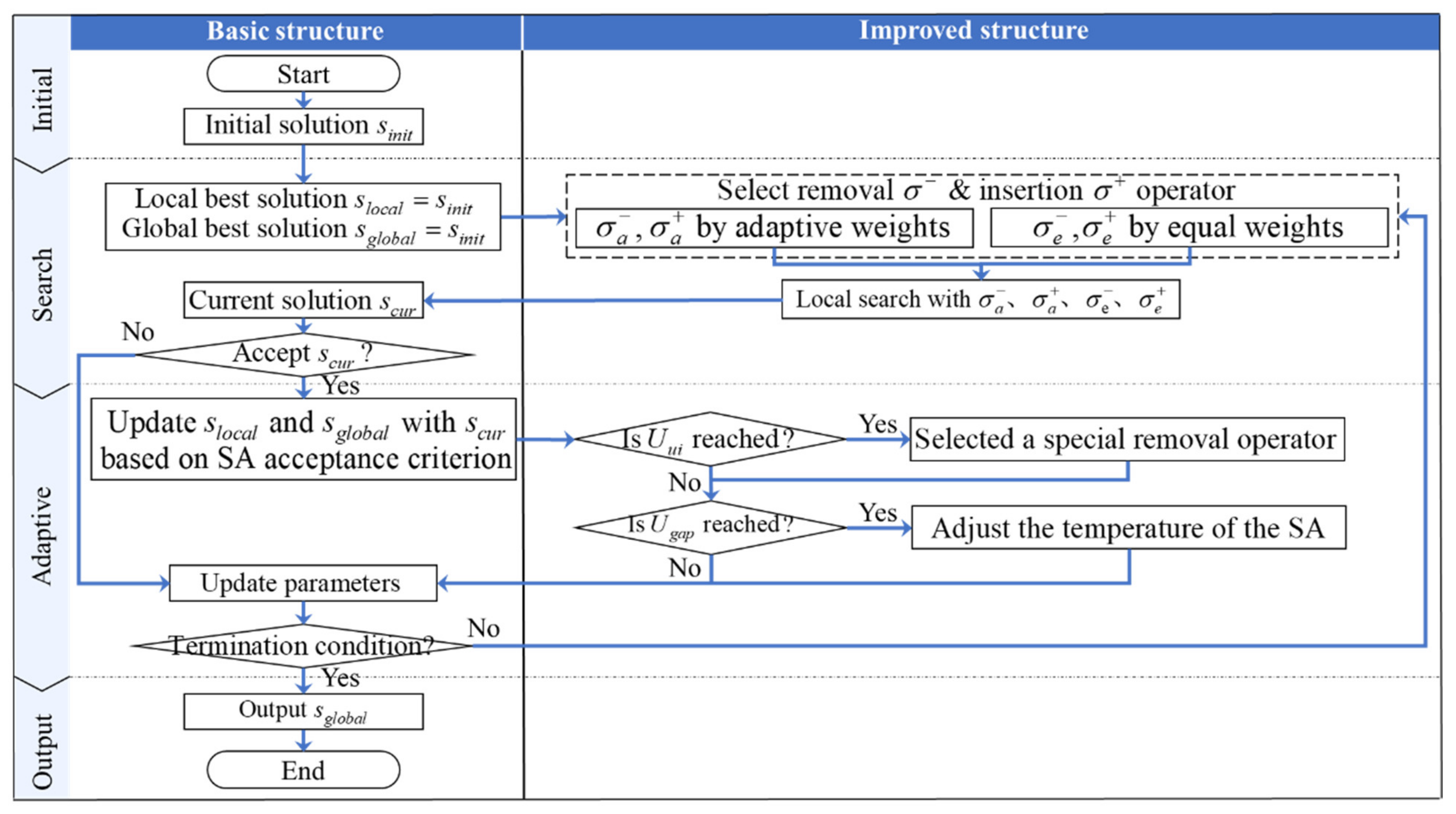
Figure 3 introduces the structure of MSALNS. Construct the initial solution by greedy insertion. Based on the initial solution, MSALNS performs removal and insertion actions on the current solution to obtain the neighborhood solution. Then, when the neighborhood solution is improved, it accepts the neighborhood solution and updates the scores of different operators.
The algorithm determines the selected removal and insertion operators based on the different scores in each generation of search. When the neighborhood solution is not improved, the solution is accepted by simulated annealing strategy. Simulated annealing is a commonly used adaptive mechanism in ALNS [
40,
41,
42,
43], as shown in
Section 4.4. Compared to other adaptive strategies, the simulated annealing approach effectively balances simplicity and efficiency. Its mechanism is straightforward and clear, while also effectively controlling the LNS in selecting different neighborhood structures. This ensures high search efficiency and helps avoid getting trapped in local optima, thus ensuring the quality of the solution.
In order to improve the ability of the algorithm to jump out of the local optimal solution, the following new strategies are designed:
If the number of times () that the solution has not been updated reaches the threshold , a random removal operator and a random repair operator are selected to destroy the current solution on a larger scale.
If the number of times () that the simulated annealing reaches the threshold , is reinitialized as to increase the probability of accepting a poor solution.
In each generation of the search, equal weights and adaptive weights based on operator scores are applied. Both methods perform the search, and the better solution is accepted.
The main improvements of the proposed algorithm are as follows:
Design of different operators (e.g., satisfaction-based Shaw removal, worst-route satisfaction removal, location-related removal, sequence-related removal, and satisfaction-based best insertion) to enrich the neighborhood structure, as shown in
Section 4.3.
Adoption of a dual-weight local search strategy to balance the influence of historical and recent performance in selecting neighborhood structures, as shown in
Section 4.4.
A simulated annealing-inspired acceptance criterion is designed, and a temperature adaptation strategy is proposed, which allows the temperature to rise when the search becomes stagnant, thus preventing the algorithm from prematurely converging to local optima.
4.1. Solution Representation for Delivery Options
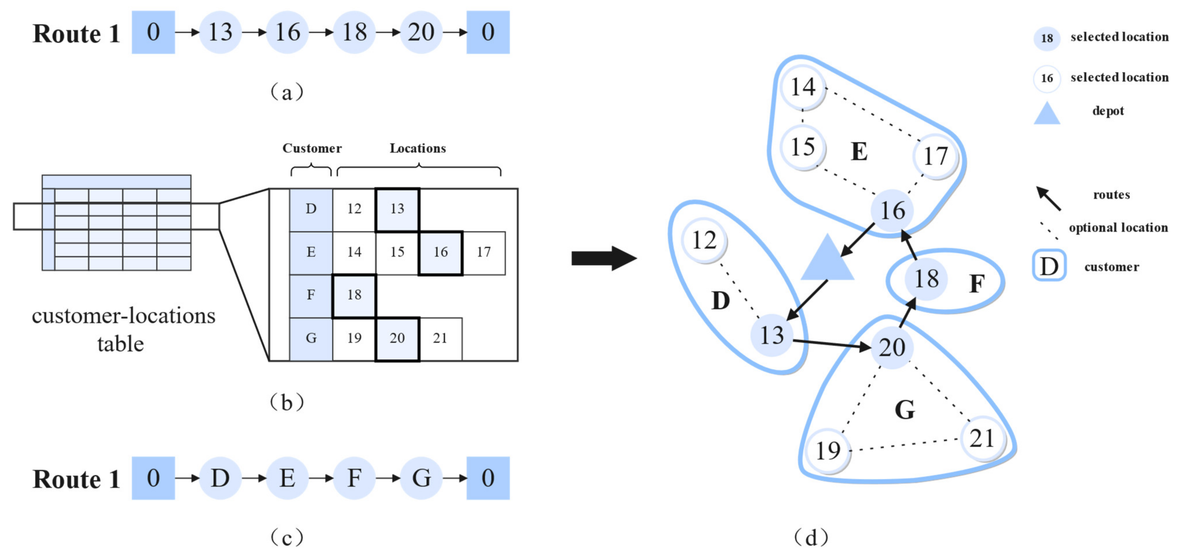
In MSALNS, a solution representation is designed based on integer encoding. Each vehicle
is associated with two strings. Assume that vehicle
needs to serve customers
. The optional service locations for these customers are
. The first location string includes the visited delivery locations and the order of the visits, as shown in
Figure 4a, which can be represented by
. The second customer string includes the visited customers and the order of the visits, as shown in
Figure 4c, which can be represented by
. A customer-location table is used to represent the optional delivery locations of a customer, as shown in
Figure 4b.
4.2. The Initial Feasible Solution
The initial solution is obtained by iteratively constructing feasible routes using a greedy strategy and a fast insertion heuristic, as shown in Algorithm 1.
| Algorithm 1. Pseudo code of initial phase |
![Applsci 15 04995 i001]() |
represents the set of customers that have not yet been assigned into a route. The algorithm randomly takes a customer at a time to build the current path . Path is initially an empty path, and each time customer is scheduled to be served at the end of . Note that a new path is generated for each optional delivery location of customer . Record the feasible with , and then through greedy strategy, choose the location with the lowest service cost as the delivery location of customer . When the path fails to serve customer , the algorithm records into the current solution and then clears the path to continue scheduling the remaining customers in . Finally, is output as the initial solution .
4.3. The Search Mechanism
Starting from an initial feasible solution, multiple removal and insertion operators in MSALNS effectively expand the neighborhood range, extend the search space, and generate higher-quality solutions.
4.3.1. Removal Operators
The removal operators destroy the structure of a part of the solution by selecting it randomly or based on a specific criterion. In this way, a certain amount of “free space” is created for subsequent optimization.
MSALNS can achieve a sizable neighborhood using a variety of removal operations. After removal, customers are placed in the request bank. The removal operator selects
customers from the current solution to perform removal. Then, the current solution becomes a partial solution.
Figure 5 is an illustration of removal operators.
MSALNS uses some of the operators that are widely used in the VRP with time windows problems. Specifically, random removal [
44], time-related removal [
45], random route removal [
44], route removal [
46], worst cost removal [
47], zone removal [
48]. MSALNS adjusts these operators according to the characteristics of the VRP-CS.
However, these operators do not consider the characteristics of the VRP-CS, optional delivery locations, and customer satisfaction. Moreover, they do not take full advantage of the degree of similarity between different delivery routes. Therefore, in order to expand the search space, improve the search performance, and the ability of the algorithm to jump out of the local optimal solution, MSALNS presents the following new operators:
- 4.
Satisfaction Shaw Removal: In this destruction operator, a reference customer location
is first randomly selected, and then the similarity between the other locations in the current solution and
is calculated. Then, it deletes
and a number of locations that are most similar to
until
locations are deleted. Specifically, for the current location
, the relationship
between the two is calculated as follows:
where
represents the distance between delivery options
and
;
and
represent the demand of customer
,
;
represents the customer satisfaction of customer
receiving service at
;
represents the customer satisfaction of customer
receiving service at
;
indicates whether customer
and
are delivered by the same vehicle; if so,
; otherwise
.
,
,
,
,
are the weight of each parameter in the formula. A lower
indicates a greater similarity between customers.
- 5.
Worst Route Satisfaction Removal: This operator calculates the total satisfaction of each route from the perspective of the route, selects the route in ascending order, and deletes all locations with low satisfaction until the number of locations removed reaches .
- 6.
Location Related Removal: This operator preferentially removes customers with similar optional locations.
- 7.
String Related Removal: This operator uses the distance between locations as a basis for judgment. First, a customer location is randomly selected as a reference location, and nearest points to it on the same route are deleted. Then, it selects a nearest point that is not on the same route and deletes nearest point to it on that route.
4.3.2. Insertion Operators
The insertion operators reinsert destroyed parts by means of random, heuristic, or local search. It aims to improve the quality of the solution. The design of the insertion operation can affect the quality of the solution and is therefore usually adapted to the characteristics of the problem.
In MSALNS, customers in are fixed to a partial solution using the insert operator. The insert operator performs only viable inserts. The insertion operators perform only feasible insertions.
Figure 6 is an example illustrating how to calculate the different insertion metrics of customer H. The darker colors are used to indicate better metric values.
In MSALNS, the classical operator random insertion [
49], greedy insertion, and cost regret insertion [
44] are adapted. At the same time, in order to better construct high-quality neighborhood solutions, MSALNS constructs the following operators from the perspective of customer satisfaction:
4.4. The Adaptive Mechanism
For the selection of different removal and insertion operators, a roulette mechanism is used. For all operators, the initial score is set to 1, and the score of different operators is increased according to the use of operators in each search process. It should be noted that the probability of selecting different operators depends on their score. The scores of the operators used to generate are updated based on the outcome, using the following reward scheme designed to favor operators that lead to better solutions:
If is a new global best solution (), the operators involved receive the highest reward .
If improves upon the current local best () but is not a new global best, they receive .
If is worse than () but is still accepted by the SA criterion, they receive .
If is worse and not accepted, they receive the lowest reward .
The operator score is updated at the end of each iteration interval, with the interval length being 50 generations. While retaining appropriate historical experience, the search test of the previous iteration interval is fully considered. The updated formula is as follows:
where
represents the scores of operators for the
iteration interval,
represents the scores accumulated by the operators between the corresponding
iteration intervals, and
represents the decay factor. The selection weights of different operators are calculated as follows during each iteration search:
where
represents its weight,
represents its score, and
represents the set of operators of the same type.
To balance exploration and exploitation within each iteration, MSALNS performs a dual search. It executes sub-searches where removal/insertion operators are chosen with equal probability, and another sub-searches where operators are chosen adaptively based on their current weights (calculated using Equation (17) from scores updated via Equation (16)), where is a parameter defining the number of searches per strategy. The best solution found among all generated neighbors become the candidate solution for potential acceptance. Furthermore, to prevent the search from stagnating, if the global best solution has not improved for iterations, the simulated annealing temperature is reset to its initial value , increasing the likelihood of accepting diversifying moves.
5. Results and Discussion
The numerical experiments run on a Microsoft Windows 11 operating system with a 12th Gen Intel(R) Core (TM) i7-12700H processor and 16 GB of RAM, and they were coded in Python 3.10. The MILP model was solved using the Gurobi 10.0.2 solver, and the IDE used for the MSALNS algorithm was PyCharm 2022.2.3.
5.1. Datasets and Parameter Setting
In the VRP-CS, the instances are generated based on the VRPRDL dataset [
28]. A psychological reference point related to delivery time is assigned to each optional delivery location. For location
, the values of the psychological reference point are randomly assigned between
and
according to a Gaussian distribution. All instances are self-explanatory, i.e., they are named according to the number of customers and total number of locations. For example, for a dataset with 20 customers and 62 optional locations, the instance is named C21L62. Instances of four sizes are designed with 16, 21, 31, and 61 customers, respectively.
This VRP-CS problem uses the risk attitude coefficient
, proposed by Kahneman and Tversky [
50], and, at the same time, sets the loss of aversion coefficient
. The value of the determined parameters is selected by means of a controlled experiment. The unit cost of delivery time is 1; the cost of using a single vehicle is 20; and the cost of unit customer satisfaction is 20. The MSALNS algorithm depends on the following parameters: maximum number of iterations
, number of iterations without improvement
, number of iterations for updating the annealing temperature
, score attenuation coefficient
, cooling rate
, initial score
, score value of the reward
,
,
,
, satisfaction Shaw removal operator coefficient
,
,
,
,
, and the scale coefficient of the removal operator
. Through comparative experiments, all the MSALNS parameters set are shown in
Table 1.
5.2. Algorithm Analysis
In MSALNS, experimental verification is conducted on the design examples. First, Gurobi is used to obtain exact solutions for the instances, which serve as a benchmark to compare and verify the quality of the algorithm solutions. Subsequently, the algorithm is compared with different meta-heuristic algorithms on the instances to demonstrate its performance through the approximate solutions obtained from these comparisons.
5.2.1. Comparisons with Gurobi
Gurobi has a large limitation on the scale of the problem to be solved. To benchmark MSALNS against exact solutions, we compared it with the Gurobi solver on smaller problem instances, as Gurobi’s runtime becomes prohibitive on the full datasets. These smaller instances, reported in
Table 2, were derived from two of the larger base datasets (C16L62 and C21L80). Specifically, for each base dataset, three smaller test cases are created by selecting only the first 5, first 10, and first 15 customers, respectively, along with the depot and all associated optional delivery locations for the selected customers. For example, the instance labeled “C16L62-10” in
Table 2 consists of the depot and the first 10 customers listed in the original C16L62 dataset.
The performance comparison with Gurobi’s solution results for these examples is shown in
Table 2. In this table, the first column represents the different instances; the second column represents the number of optional locations; the third column,
Best, represents the best solution cost found by MSALNS;
Avg. represents the average solution cost found by MSALNS;
Gap represents the difference between
Best and
Avg.; and
Time represents the fastest running time of MSALNS. In the fourth column,
Best represents the exact solution cost found by Gurobi, and
Time represents the time taken by Gurobi to find the solution. The formula for calculating
is as follows:
where
represents the cost of the best solution obtained by MSALNS and
represents the cost of the best solution obtained by Gurobi.
The results show that the proposed MSALNS can obtain a solution that is close to the exact solution of Gurobi, and, at the same time, the solution time has been significantly improved. Moreover, this proves the correctness of our proposed VRP-CS model. However, considering that the optional locations increase the complexity of the problem, when the number of customers increases to 16, the Gurobi solver cannot solve these problems on the device.
5.2.2. Comparisons with Meta-Heuristic Algorithms
For the examples that are difficult to solve with exact methods such as Gurobi, further analysis is needed to evaluate the performance of MSALNS. Therefore, a comparative analysis was performed on all instances using the proposed MSALNS and three other metaheuristic algorithms: a standard Adaptive Large Neighborhood Search (ALNS), the Tunicate Swarm Algorithm (TSA, Kaur et al. [
51]), and the Sand Cat Swarm Optimization (SCSO, Seyyedabbasi and Kiani, [
52]).
The algorithms selected for comparison include:
ALNS: This represents the standard Adaptive Large Neighborhood Search framework, upon which our MSALNS is built. The ALNS does not include the specific improvements introduced in our MSALNS, such as the satisfaction-based operators, dual-weighted local search, or the secondary simulated annealing restart mechanism.
TSA (Tunicate Swarm Algorithm): TSA is a recent bio-inspired metaheuristic algorithm that mimics the survival behaviors of tunicates in the ocean. It models two key aspects: the jet propulsion used by individual tunicates for movement (including mechanisms to avoid conflicts between individuals and move towards the best neighbor) and the swarm intelligence that updates the positions of search agents relative to the best-found solutions so far.
SCSO (Sand Cat Swarm Optimization): SCSO is another nature-inspired algorithm based on the survival strategies of sand cats in deserts. The algorithm models two main behaviors derived from the sand cat’s hunting techniques: searching for prey (exploration phase), inspired by the cat’s ability to detect low-frequency sounds to locate prey, and attacking the prey (exploitation phase), guided by the cat’s position relative to the prey. The algorithm uses adaptive parameters to balance these two phases.
The effectiveness of the algorithm improvements can be evaluated by comparing MSALNS with the standard ALNS. Additionally, comparisons with two recent swarm intelligence algorithms, TSA and SCSO, provide further insights into the performance of MSALNS relative to other recent metaheuristic algorithms.
For the TSA and SCSO algorithms, the number of iterations is set to 500, and the number of populations is set to 100. To verify the performance of MSALNS, the four algorithms are verified on different datasets with 16, 21, 31, and 61 customers, respectively.
The performance comparison results of the algorithms are shown in
Table 3. For each algorithm, the best solution cost and coefficient of variation in the solution are calculated by the calculation 10 times. The first column represents the different instances used, and the second column represents the best solution cost, coefficient of variation, and solving time (the unit is second) of the solution found in the MSALNS method. The third, fourth, and fifth columns are similar and represent the corresponding parameters of the ALNS, TSA, and SCSO algorithms.
The experimental results show that MSALNS has a significant improvement effect on ALNS. MSALNS can find the best solution in 20 instances, and only in 3 instances with fewer customers is the best solution obtained by TSA and SCSO. At the same time, our MSALNS fully expands the search range, and the solution quality can be basically controlled within 10%, showing good stability. At the same time, in all instances, we can see that MSALNS has been effectively improved compared to the basic ALNS. The experimental results show that MSALNS achieves this significant improvement in solution quality (compared to ALNS) with comparable computational effort (see average run times in
Table 3). While TSA and SCSO were generally slower, MSALNS demonstrates a strong balance between effectiveness and efficiency for the VRP-CS.
In
Figure 7, the red line represents the median and the blue line represents the mean. When the number of customers is 15, the performance of MSALNS is not much different from that of other algorithms. When the number of customers increases, MSALNS shows better solving ability. In the examples of 20, 30, and 60 customers, MSALNS performs best. Comparing these four algorithms, MSALNS and basic ALNS perform better than TSA and SCSO. MSALNS has similar stability to that of basic ALNS, while TAS and SCSO have poor stability.
MSALNS outperforms ALNS, TSA, and SCSO in both solution quality and computational time. MSALNS introduces removal and insertion operators based on satisfaction-oriented delivery construction and designs an adaptive dual sub-search mechanism combined with a multi-annealing strategy. These improvements address a gap in the existing literature, where most previous studies either simplified the modeling of customer satisfaction or treated delivery options as static constraints. By simultaneously considering flexible delivery choices and satisfaction objectives, MSALNS achieves optimization results that better align with customer preferences.
5.3. Evaluation of Question Features
In this section, the impact of different problem characteristics on the total cost is analyzed. First, the impact of customer satisfaction as a comprehensive goal is considered. Second, the impact of using optional delivery locations on the various cost is analyzed.
5.3.1. The Effect of Customer Satisfaction
To investigate the impact of customer satisfaction on the solution, the MSALNS was run on all instances with and without customer satisfaction. In each case, MSALNS is run 10 times on the instance. The satisfaction and delivery cost of the solution are shown in
Table 4 and
Figure 8.
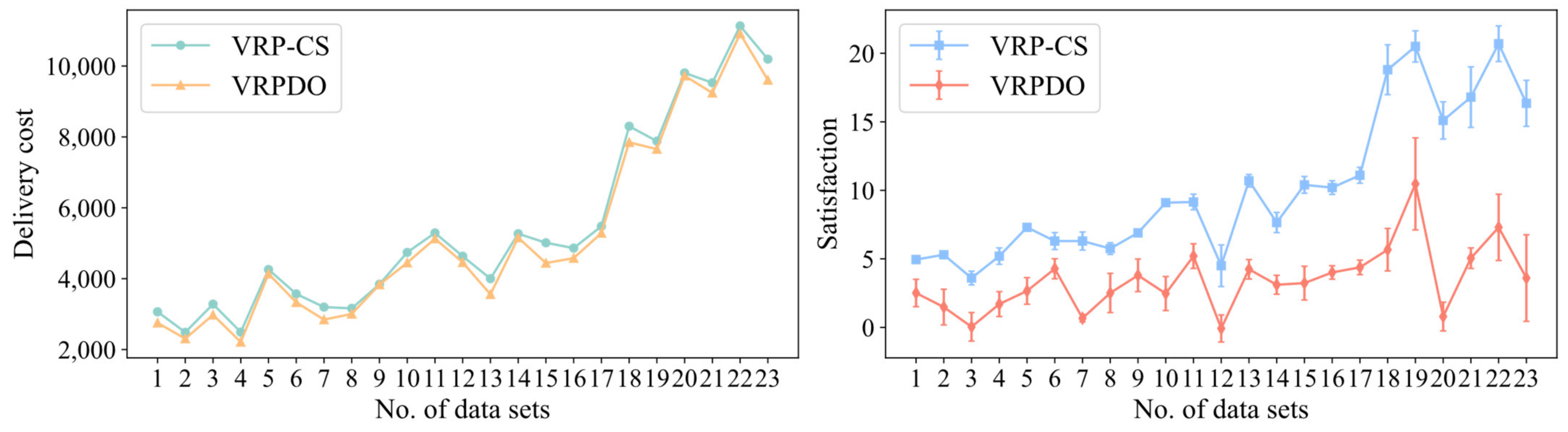
Table 4 shows the comparison experiment considering customer satisfaction and not considering customer satisfaction. We call the case where customer satisfaction is considered the VRP-CS and the case where customer satisfaction is not considered the VRPDO. The first column shows the instance we use; the second column shows the experimental results in the VRP-CS case;
represents the corresponding delivery cost; and
represents the corresponding customer satisfaction. The third column shows the corresponding results of VRPDO and the corresponding parameter gap. We use
and
to represent the corresponding value gap, and the calculation formula for
is as follows:
where
indicates the parameters that take customer satisfaction into account, and
indicates the parameters that do not take customer satisfaction into account. For distribution cost,
and
are both calculated using the corresponding
. For customer satisfaction, we use
to represent the situation where all customers are completely dissatisfied.
and
are both calculated using the corresponding
. It should be noted that a positive
indicates that the MSALNS solution has a lower distribution cost and higher customer satisfaction, while a negative
indicates the opposite.
When considering customer satisfaction, the average delivery cost loses 5.68%, while the average customer satisfaction increases by 15.32%. In terms of delivery cost, the VRP-CS performs worse than the VRPDO across all instances. Specifically, in 6 instances, the difference in delivery cost between the VRP-CS and the VRPDO is around 10%, while in the other 17 instances, the difference is around 5% or less, indicating a relatively small gap. However, in terms of total customer satisfaction, the VRP-CS shows a significant improvement. In 22 cases, the VRP-CS improved its total customer satisfaction by at least 12%. In
Figure 8, the standard deviation is used to represent the error. By taking customer satisfaction into account, the stability of the VRP-CS’s target satisfaction plan is better than that of the VRPDO.
5.3.2. The Effect of Delivery Options
In each instance, MSALNS operates 10 times with or without consideration of optional delivery locations. For different cases, the case with delivery options is called the VRP-CS and the case with a single delivery location is called the VRPSD.
As shown in
Table 5, the first column represents the instances used; the second column represents the average total cost
found by the algorithm in the VRP-CS case, the average delivery cost
and the corresponding average customer satisfaction
; and the third column represents the corresponding items in the VRPSD case. In addition, we further use
and
to represent the numerical difference between the corresponding parameters. The calculation method is similar to that of Formula (19). Note that for
and
, a negative
indicates that the VRPDO has achieved a better solution, and for
, a positive
indicates that the VRPDO has achieved a better solution.
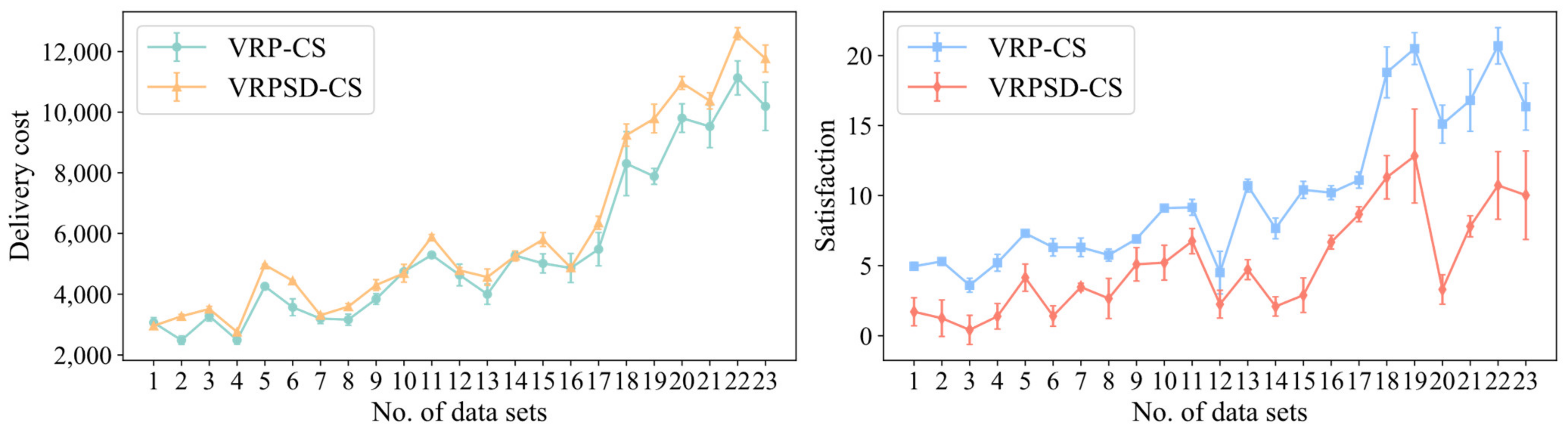
Through experimental data, the VRP-CS with delivery options offers greater flexibility in logistics and distribution. Remarkable results have been achieved in reducing distribution cost and improving customer satisfaction. The total cost of the VRP-CS is reduced by an average of 14.22%. In only one instance, the total cost of the VRP-CS is 0.81% higher than that of the VRPSD, its delivery cost is 3.46% higher, but its customer satisfaction is 16.23% higher. The VRP-CS has an average increase in customer satisfaction of 12.37%, indicating that the VRP-CS with delivery options effectively improves customer satisfaction. The VRP-CS delivery cost has been reduced by an average of 11.30%. In only three instances does the VRP-CS cost more to deliver than VRPSD, but the difference is within 3.5%. In
Figure 9, standard deviation is used to represent the error. In terms of delivery cost, there is some volatility in the VRP-CS solutions due to delivery options and satisfaction. In terms of satisfaction, the VRP-CS solution is stable and can achieve better satisfaction.
The VRP-CS improves customer satisfaction with only a slight increase in delivery cost (
Table 4), demonstrating the effectiveness of the proposed satisfaction-oriented optimization approach and solving the limitations of the simple strategies discussed in
Section 2.1. In addition, the use of delivery options improves customer satisfaction while reducing costs (
Table 5), highlighting the advantages of flexible delivery strategies, as discussed in
Section 2.2.
The results show that by considering customer satisfaction, the VRP-CS sacrifices only about 5% of delivery cost while achieving approximately a 15% improvement in customer satisfaction. Moreover, by adopting a delivery model with flexible options, the total cost is reduced by 14.22%; delivery cost is reduced by 11.3%; and customer satisfaction increases by 12.37%.
6. Conclusions
A Vehicle Routing Problem considering Customer Satisfaction (VRP-CS) is studied, where customer preferences for delivery time and location are incorporated. Satisfaction is evaluated using prospect theory, and a MSALNS algorithm is developed to address the resulting bi-objective optimization. Numerical experiments yielded several key findings:
The proposed MSALNS algorithm demonstrated superior performance compared to standard ALNS, TSA, and SCSO on the VRP-CS benchmark instances, finding better solutions in the majority of cases.
By adopting a prospect theory-based customer satisfaction evaluation method, the VRP-CS achieves an average improvement of 15.32% in customer satisfaction, with only a 5.68% increase in delivery cost. This indicates that service quality and customer satisfaction can be effectively improved with a controllable increase in cost.
Utilizing optional delivery locations led to substantial benefits, reducing average total costs by 14.22% and delivery costs by 11.30%, while simultaneously increasing average customer satisfaction by 12.37%.
These findings demonstrate the effectiveness of the VRP-CS in achieving a balanced trade-off between delivery cost and customer satisfaction.
This paper proposes a mathematical model that considers customer satisfaction and alternative delivery locations. In view of the complexity of the problem, an MSALNS algorithm is designed, introducing some new strategies that jump out of local optimal, adapting some classic and effective removal and insertion operators, and designing some new removal and insertion operators that consider customer satisfaction to reconstruct solutions to expand the search space. In addition, new efficient removal operators are introduced to accelerate the convergence of MSALNS. Numerical experiments are used to verify the efficiency and effectiveness of the MSALNS algorithm and to analyze the impact of customer satisfaction on delivery cost as well as the impact of optional delivery locations on delivery cost and customer satisfaction.
This study has several limitations, which also point to directions for future research. The current VRP-CS assumes deterministic travel and service times, ignoring real-world factors such as traffic conditions, which may affect the feasibility of routes and the accuracy of customer satisfaction evaluation. The parameters (α, β, λ) in the prospect theory function are adopted from recommended values in the existing literature, without being tailored to individual customer characteristics, which limits the precision of the satisfaction assessment. In addition, computational experiments are conducted on simulated datasets. To fully evaluate the practical significance of the VRP-CS in real-world logistics distribution, it is necessary to validate the approach using large-scale real-world data from logistics companies.
To address the limitations of the VRP-CS, future research can focus on several directions. One direction is to develop a stochastic VRP-CS model that explicitly considers uncertainty in travel time or customer service time, thereby enhancing the robustness of the solution. Another is to improve the accuracy of customer satisfaction evaluation by incorporating real customer feedback or historical delivery data, potentially through reinforcement learning or other data-driven methods. Further, additional factors influencing customer satisfaction—such as the demand for delivery consistency—could be included to enrich the satisfaction evaluation framework. Finally, validating the VRP-CS using real-world datasets is of great importance. From an algorithmic perspective, exploring alternative optimization techniques, such as constraint programming combined with LNS (CP-LNS) or reinforcement learning-based methods, could help strike a better balance between solution quality and computational effort.
Author Contributions
Conceptualization, X.D. and X.Z.; funding acquisition, X.Z. and P.L.; investigation, X.D. and P.L.; methodology, X.D. and J.H.; project administration, J.H.; supervision, X.Z. and J.H.; validation, P.L. and J.H.; writing—original draft, X.D.; writing—review and editing, X.Z. and P.L. All authors have read and agreed to the published version of the manuscript.
Funding
This research was funded by the Natural Science Foundation of Hubei Province of China under Grant 2025AFA055 and the National Key Research and Development Program of China under Grant 2020YFB1710804.
Institutional Review Board Statement
Not applicable.
Informed Consent Statement
Not applicable.
Data Availability Statement
Some or all data and code that support the findings of this study are available from the corresponding author upon reasonable request.
Acknowledgments
The authors are grateful to the subjects for their contributions to the experiment.
Conflicts of Interest
The authors declare no conflicts of interest.
Abbreviations
The following abbreviations are used in this manuscript:
| VRP-CS | Vehicle routing problem considering customer satisfaction |
| NP-hard | A computational problem H is called NP-hard if, for every problem L which can be solved in non-deterministic polynomial-time, there is a polynomial-time reduction from L to H |
| LNS | Large Neighborhood Search |
| ALNS | Adaptive Large Neighborhood Search |
| MSALNS | Multi-Strategies Adaptive Large Neighborhood Search |
| VRP | Vehicle routing problem |
| VRPDO | Vehicle routing problem with delivery options |
| VRPRDL | Vehicle routing problem with roaming delivery locations |
| VRPSD | The special case of the VRP-CS where each customer has only one delivery option |
| TSA | Tunicate Swarm Algorithm |
| SCSO | Sand Cat Swarm Optimization |
| SA | Simulated Annealing |
Appendix A
Appendix A.1
This section lists the indices and parameters used in the mathematical formulation of the VRP-CS model.
Table A1.
Indices.
| Symbol | Description |
|---|
| Depot (Hub) |
| A set of customers, |
| A set of customers and depots, |
| A set of Vehicle, |
| A set of optional delivery locations for all customers, , is the optional delivery location of depot |
| A set of optional delivery locations for customer , |
Table A2.
Parameters.
| Symbol | Description |
|---|
| The a-th optional delivery location of customer () |
| Distance between delivery points ,(,) |
| Travel cost per unit distance of vehicle |
| Cost of travel between points ,(,) |
| Demand of customer () |
| Time window for customer ’s a-th optional delivery location |
| The psychological reference point for customer to be satisfied at the a-th optional delivery location |
| Service time of customer |
| Time limit for vehicles |
| Distance limit for vehicles |
| Penalty cost per unit of customer satisfaction |
| Operating cost of vehicles |
| Capacity limit for vehicles |
| Average speed of the vehicle |
| A sufficiently large positive number |
References
- Barenji, A.V.; Wang, W.M.; Li, Z.; Guerra-Zubiaga, D.A. Intelligent E-Commerce Logistics Platform Using Hybrid Agent Based Approach. Transp. Res. Part E Logist. Transp. Rev. 2019, 126, 15–31. [Google Scholar] [CrossRef]
- Zhao, S.; Li, P.; Li, Q. The Vehicle Routing Problem Considering Customers’ Multiple Preferences in Last-Mile Delivery. Teh. Vjesn. 2024, 31, 734–743. [Google Scholar] [CrossRef]
- Niu, X.Y.; Liu, S.F.; Huang, Q.L. End-of-Line Delivery Vehicle Routing Optimization Based on Large-Scale Neighbourhood Search Algorithms Considering Customer-Consumer Delivery Location Preferences. Adv. Prod. Eng. Manag. 2022, 17, 439–454. [Google Scholar] [CrossRef]
- Hamzah, A.A.; Shamsudin, M.F. Why Customer Satisfaction Is Important to Business? J. Undergrad. Soc. Sci. Technol. 2020, 2, 1–14. [Google Scholar]
- Ma, X.; Bian, W.; Wei, W.; Wei, F. Customer-Centric, Two-Product Split Delivery Vehicle Routing Problem under Consideration of Weighted Customer Waiting Time in Power Industry. Energies 2022, 15, 3546. [Google Scholar] [CrossRef]
- Ghannadpour, S.F.; Noori, S.; Tavakkoli-Moghaddam, R. Multiobjective Dynamic Vehicle Routing Problem With Fuzzy Travel Times and Customers’ Satisfaction in Supply Chain Management. IEEE Trans. Eng. Manag. 2013, 60, 777–790. [Google Scholar] [CrossRef]
- Zhou, L.; Zhong, S.; Ma, S.; Jia, N. Prospect Theory Based Estimation of Drivers’ Risk Attitudes in Route Choice Behaviors. Accid. Anal. Prev. 2014, 73, 1–11. [Google Scholar] [CrossRef]
- Li, W.; Zhang, Q.; Huang, M.; Yu, Y. Multi-Depot Vehicle Routing Problem Considering Customer Satisfaction. In Proceedings of the 2021 33rd Chinese Control and Decision Conference (CCDC), Kunming, China, 22–24 May 2021; pp. 4208–4213. [Google Scholar]
- Zhang, J.; Li, Y.; Lu, Z. Multi-Period Vehicle Routing Problem with Time Windows for Drug Distribution in the Epidemic Situation. Transp. Res. Part C Emerg. Technol. 2024, 160, 104484. [Google Scholar] [CrossRef]
- Shaw, N.; Eschenbrenner, B.; Baier, D. Online Shopping Continuance after COVID-19: A Comparison of Canada, Germany and the United States. J. Retail. Consum. Serv. 2022, 69, 103100. [Google Scholar] [CrossRef]
- Dantzig, G.B.; Ramser, J.H. The Truck Dispatching Problem. Manag. Sci. 1959, 6, 80–91. [Google Scholar] [CrossRef]
- Costa, L.; Contardo, C.; Desaulniers, G.; Pecin, D. Selective Arc-ng Pricing for Vehicle Routing. Int. Trans. Oper. Res. 2021, 28, 2633–2690. [Google Scholar] [CrossRef]
- Madelin, G.; Lahrichi, N. Modeling and Improving the Logistic Distribution Network of a Hospital. Int. Trans. Oper. Res. 2021, 28, 70–90. [Google Scholar] [CrossRef]
- Erdoğdu, K.; Karabulut, K. Bi-objective Green Vehicle Routing Problem. Int. Trans. Oper. Res. 2022, 29, 1602–1626. [Google Scholar] [CrossRef]
- Fröhlich, G.E.A.; Gansterer, M.; Doerner, K.F. Safe and Secure Vehicle Routing: A Survey on Minimization of Risk Exposure. Int. Trans. Oper. Res. 2023, 30, 3087–3121. [Google Scholar] [CrossRef]
- Fan, J. The Vehicle Routing Problem with Simultaneous Pickup and Delivery Based on Customer Satisfaction. Procedia Eng. 2011, 15, 5284–5289. [Google Scholar] [CrossRef]
- Qin, G.; Tao, F.; Li, L. A Vehicle Routing Optimization Problem for Cold Chain Logistics Considering Customer Satisfaction and Carbon Emissions. Int. J. Environ. Res. Public Health 2019, 16, 576. [Google Scholar] [CrossRef]
- Afshar-Bakeshloo, M.; Mehrabi, A.; Safari, H.; Maleki, M.; Jolai, F. A Green Vehicle Routing Problem with Customer Satisfaction Criteria. J. Ind. Eng. Int. 2016, 12, 529–544. [Google Scholar] [CrossRef]
- Yu, X.-P.; Hu, Y.-S.; Wu, P. The Consistent Vehicle Routing Problem Considering Driver Equity and Flexible Route Consistency. Comput. Ind. Eng. 2024, 187, 109803. [Google Scholar] [CrossRef]
- Su, Y.; Zhang, S.; Zhang, C. A Lightweight Genetic Algorithm with Variable Neighborhood Search for Multi-Depot Vehicle Routing Problem with Time Windows. Appl. Soft Comput. 2024, 161, 111789. [Google Scholar] [CrossRef]
- Yue, B.; Ma, J.; Shi, J.; Yang, J. A Deep Reinforcement Learning-Based Adaptive Search for Solving Time-Dependent Green Vehicle Routing Problem. IEEE Access 2024, 12, 33400–33419. [Google Scholar] [CrossRef]
- Xu, S.; Ou, X.; Govindan, K.; Chen, M.; Yang, W. An Adaptive Genetic Hyper-Heuristic Algorithm for a Two-Echelon Vehicle Routing Problem with Dual-Customer Satisfaction in Community Group-Buying. Transp. Res. Part E Logist. Transp. Rev. 2025, 194, 103874. [Google Scholar] [CrossRef]
- Stavropoulou, F. The Consistent Vehicle Routing Problem with Heterogeneous Fleet. Comput. Oper. Res. 2022, 140, 105644. [Google Scholar] [CrossRef]
- Cui, H.; Qiu, J.; Cao, J.; Guo, M.; Chen, X.; Gorbachev, S. Route Optimization in Township Logistics Distribution Considering Customer Satisfaction Based on Adaptive Genetic Algorithm. Math. Comput. Simul. 2023, 204, 28–42. [Google Scholar] [CrossRef]
- Zheng, K.; Huo, X.; Jasimuddin, S.; Zhang, J.Z.; Battaïa, O. Logistics Distribution Optimization: Fuzzy Clustering Analysis of e-Commerce Customers’ Demands. Comput. Ind. 2023, 151, 103960. [Google Scholar] [CrossRef]
- Wang, Z.; Liu, J.; Zhang, J. Hyper-Heuristic Algorithm for Traffic Flow-Based Vehicle Routing Problem with Simultaneous Delivery and Pickup. J. Comput. Des. Eng. 2023, 10, 2271–2287. [Google Scholar] [CrossRef]
- Huang, M.; Liu, M.; Kuang, H. Vehicle Routing Problem for Fresh Products Distribution Considering Customer Satisfaction through Adaptive Large Neighborhood Search. Comput. Ind. Eng. 2024, 190, 110022. [Google Scholar] [CrossRef]
- Reyes, D.; Savelsbergh, M.; Toriello, A. Vehicle Routing with Roaming Delivery Locations. Transp. Res. Part C Emerg. Technol. 2017, 80, 71–91. [Google Scholar] [CrossRef]
- Ozbaygin, G.; Ekin Karasan, O.; Savelsbergh, M.; Yaman, H. A Branch-and-Price Algorithm for the Vehicle Routing Problem with Roaming Delivery Locations. Transp. Res. Part B Methodol. 2017, 100, 115–137. [Google Scholar] [CrossRef]
- Dumez, D.; Lehuédé, F.; Péton, O. A Large Neighborhood Search Approach to the Vehicle Routing Problem with Delivery Options. Transp. Res. Part B Methodol. 2021, 144, 103–132. [Google Scholar] [CrossRef]
- Ransikarbum, K.; Wattanasaeng, N.; Madathil, S.C. Analysis of Multi-Objective Vehicle Routing Problem with Flexible Time Windows: The Implication for Open Innovation Dynamics. J. Open Innov. Technol. Mark. Complex. 2023, 9, 100024. [Google Scholar] [CrossRef]
- Voigt, S.; Frank, M.; Fontaine, P.; Kuhn, H. The Vehicle Routing Problem with Availability Profiles. Transp. Sci. 2023, 57, 531–551. [Google Scholar] [CrossRef]
- Schaap, H.; Schiffer, M.; Schneider, M.; Walther, G. A Large Neighborhood Search for the Vehicle Routing Problem with Multiple Time Windows. Transp. Sci. 2022, 56, 1369–1392. [Google Scholar] [CrossRef]
- Chen, M.-C.; Yerasani, S.; Tiwari, M.K. Solving a 3-Dimensional Vehicle Routing Problem with Delivery Options in City Logistics Using Fast-Neighborhood Based Crowding Differential Evolution Algorithm. J. Ambient. Intell. Human. Comput. 2023, 14, 10389–10402. [Google Scholar] [CrossRef]
- Karimi, A.; Zhang, L.; Fackrell, M.; Thompson, R. A Multi-Objective Two-Echelon Vehicle Routing Problem with Multiple Delivery Options. Transp. Res. Procedia 2024, 79, 377–384. [Google Scholar] [CrossRef]
- Zhang, R.; Dai, Y.; Yang, F.; Ma, Z. A Cooperative Vehicle Routing Problem with Delivery Options for Simultaneous Pickup and Delivery Services in Rural Areas. Socio-Econ. Plan. Sci. 2024, 93, 101871. [Google Scholar] [CrossRef]
- Frey, C.M.M.; Jungwirth, A.; Frey, M.; Kolisch, R. The Vehicle Routing Problem with Time Windows and Flexible Delivery Locations. Eur. J. Oper. Res. 2023, 308, 1142–1159. [Google Scholar] [CrossRef]
- Chen, S.; Chen, R.; Wang, G.-G.; Gao, J.; Sangaiah, A.K. An Adaptive Large Neighborhood Search Heuristic for Dynamic Vehicle Routing Problems. Comput. Electr. Eng. 2018, 67, 596–607. [Google Scholar] [CrossRef]
- Wang, S.; Sun, W.; Huang, M. An Adaptive Large Neighborhood Search for the Multi-Depot Dynamic Vehicle Routing Problem with Time Windows. Comput. Ind. Eng. 2024, 191, 110122. [Google Scholar] [CrossRef]
- Voigt, S. A Review and Ranking of Operators in Adaptive Large Neighborhood Search for Vehicle Routing Problems. Eur. J. Oper. Res. 2025, 322, 357–375. [Google Scholar] [CrossRef]
- Voigt, S.; Frank, M.; Fontaine, P.; Kuhn, H. Hybrid Adaptive Large Neighborhood Search for Vehicle Routing Problems with Depot Location Decisions. Comput. Oper. Res. 2022, 146, 105856. [Google Scholar] [CrossRef]
- Cunha, C.B.; Massarotto, D.F.; Fornazza, S.L.; Mendes, A.B. An ALNS Metaheuristic for the Family Multiple Traveling Salesman Problem. Comput. Oper. Res. 2024, 169, 106750. [Google Scholar] [CrossRef]
- Pereira, V.G.; Alves-Junior, O.C.; Baldo, F. An Approach to Solve the Heterogeneous Fixed Fleet Vehicle Routing Problem With Time Window Based on Adaptive Large Neighborhood Search Meta-Heuristic. IEEE Trans. Intell. Transp. Syst. 2024, 25, 8148–8157. [Google Scholar] [CrossRef]
- Ropke, S.; Pisinger, D. An Adaptive Large Neighborhood Search Heuristic for the Pickup and Delivery Problem with Time Windows. Transp. Sci. 2006, 40, 455–472. [Google Scholar] [CrossRef]
- Pisinger, D.; Ropke, S. A General Heuristic for Vehicle Routing Problems. Comput. Oper. Res. 2007, 34, 2403–2435. [Google Scholar] [CrossRef]
- Nagata, Y.; Bräysy, O. A Powerful Route Minimization Heuristic for the Vehicle Routing Problem with Time Windows. Oper. Res. Lett. 2009, 37, 333–338. [Google Scholar] [CrossRef]
- Rousseau, L.-M.; Gendreau, M.; Pesant, G. Using Constraint-Based Operators to Solve the Vehicle Routing Problem with Time Windows. J. Heuristics 2002, 8, 43–58. [Google Scholar] [CrossRef]
- Demir, E.; Bektaş, T.; Laporte, G. An Adaptive Large Neighborhood Search Heuristic for the Pollution-Routing Problem. Eur. J. Oper. Res. 2012, 223, 346–359. [Google Scholar] [CrossRef]
- Christiaens, J.; Vanden Berghe, G. Slack Induction by String Removals for Vehicle Routing Problems. Transp. Sci. 2020, 54, 417–433. [Google Scholar] [CrossRef]
- Kahneman, D.; Tversky, A. Prospect Theory: An Analysis of Decision Under Risk. In Handbook of the Fundamentals of Financial Decision Making; World Scientific Handbook in Financial Economics Series; World Scientific: Singapore, 2012; Volume 4, pp. 99–127. ISBN 978-981-4417-34-1. [Google Scholar]
- Kaur, S.; Awasthi, L.K.; Sangal, A.L.; Dhiman, G. Tunicate Swarm Algorithm: A New Bio-Inspired Based Metaheuristic Paradigm for Global Optimization. Eng. Appl. Artif. Intell. 2020, 90, 103541. [Google Scholar] [CrossRef]
- Seyyedabbasi, A.; Kiani, F. Sand Cat Swarm Optimization: A Nature-Inspired Algorithm to Solve Global Optimization Problems. Eng. Comput. 2023, 39, 2627–2651. [Google Scholar] [CrossRef]
Figure 1.
An illustration of the VRP-CS. (a) Distribution routing design. (b) Delivery options of customers.
Figure 1.
An illustration of the VRP-CS. (a) Distribution routing design. (b) Delivery options of customers.
Figure 2.
Distribution of customer satisfaction.
Figure 2.
Distribution of customer satisfaction.
Figure 3.
An illustration showing the structure of MSALNS.
Figure 3.
An illustration showing the structure of MSALNS.
Figure 4.
An example solution of the VRP-CS. (a) Route of service locations. (b) Part of customer–locations table. (c) Route of service customers. (d) Distribution route.
Figure 4.
An example solution of the VRP-CS. (a) Route of service locations. (b) Part of customer–locations table. (c) Route of service customers. (d) Distribution route.
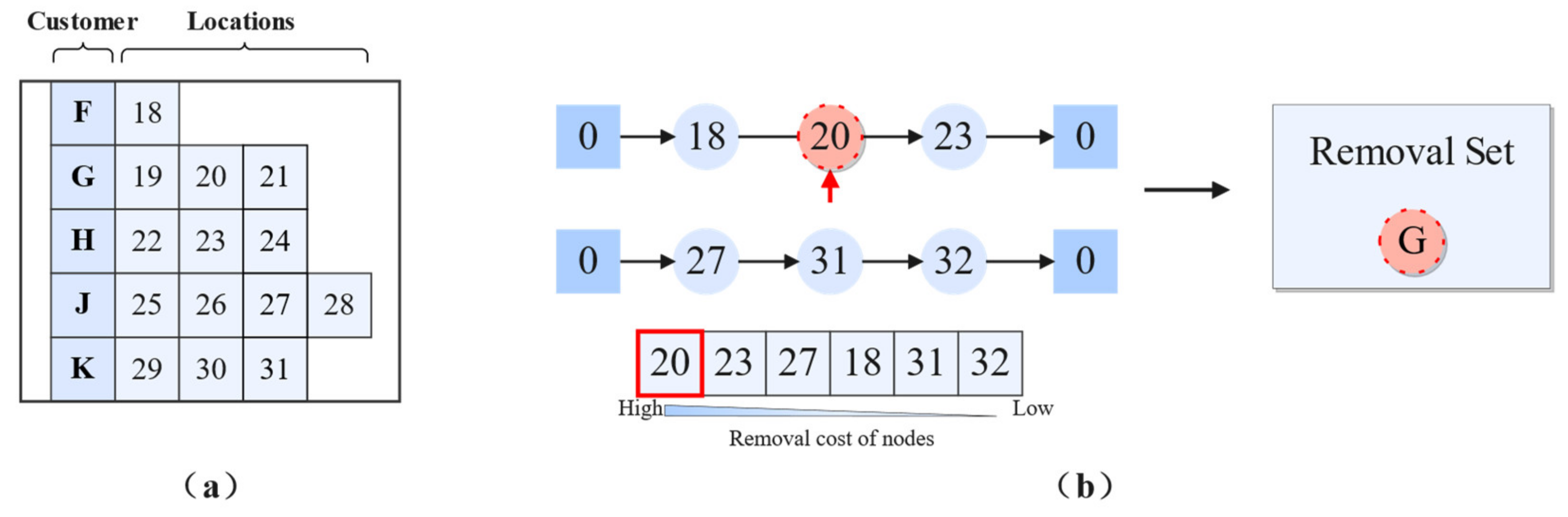
Figure 5.
Illustration of removal operators. (a) Example customer–locations table mapping customers (F–K) to potential delivery locations (18–31). (b) Schematic representation of routes where removal occurred (top panel shows two routes, with delivery locations 18, 20, 23, 27, 31, 32), delivery locations to be removed (e.g., delivery location 20), and node removal costing diagram (bottom panel), where selected customers (e.g., delivery option 20, which belongs to customer G) are moved to the “request bank” (list of removed customers).
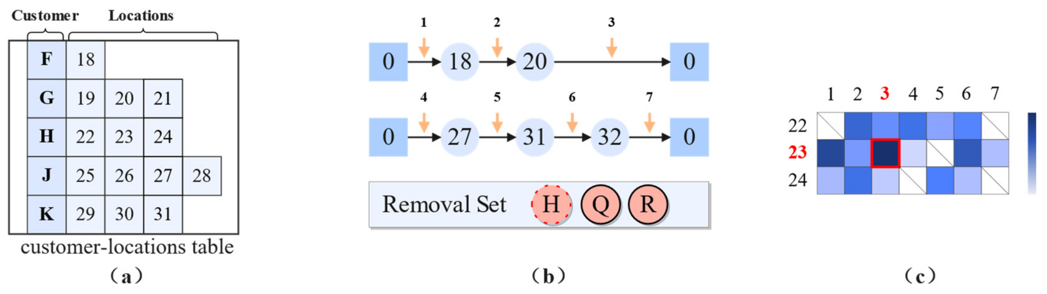
Figure 6.
An illustration of the VRP-CS. (a) Customer–locations table. (b) Index of insertable positions and removal set. (c) An illustration of the calculation of the insertion cost for customer H.
Figure 6.
An illustration of the VRP-CS. (a) Customer–locations table. (b) Index of insertable positions and removal set. (c) An illustration of the calculation of the insertion cost for customer H.
Figure 7.
Comparison of different algorithms on instances with varying customer quantities.
Figure 7.
Comparison of different algorithms on instances with varying customer quantities.
Figure 8.
Results of different sub-objectives influenced by customer satisfaction.
Figure 8.
Results of different sub-objectives influenced by customer satisfaction.
Figure 9.
Results of different sub-objectives influenced by delivery options.
Figure 9.
Results of different sub-objectives influenced by delivery options.
Table 1.
Algorithm parameter list.
Table 1.
Algorithm parameter list.
| Parameter | Value | Parameter | Value | Parameter | Value | Parameter | Value |
|---|
| 500 | | 0.992 | | 10 | | 0.5 |
| 10 | | 1 | | 5 | | 0.1 |
| 50 | | 16 | | 0.2 | | 0.3 |
| 0.3 | | 8 | | 0.2 | | 15% |
Table 2.
Performance comparison between MSALNS and Gurobi.
Table 2.
Performance comparison between MSALNS and Gurobi.
| Instance | Locs | MSALNS | | Gurobi |
|---|
| | | Best
| Avg.
| Gapbest(%) | Time (s)
| Best
| Time (s)
|
|---|
| C16L62-5 | 20 | 1394.70 | 1442.90 | 3.08% | 1.67 | 1351.69 | 28.67 |
| C16L62-10 | 43 | 1870.49 | 2078.07 | 2.35% | 3.98 | 1826.51 | 2414.4 |
| C16L62-15 | 62 | 2258.03 | 2407.51 | - | 6.06 | - | - |
| C21L80-5 | 18 | 1237.61 | 1331.66 | 3.13% | 1.89 | 1198.82 | 66.38 |
| C21L80-10 | 38 | 1785.97 | 2077.61 | 2.68% | 3.78 | 1738.19 | 2236.15 |
| C21L80-15 | 60 | 3194.04 | 3386.11 | - | 5.92 | - | - |
| Average | - | 1958.92 | 2131.72 | 2.81% | 3.88 | 1528.80 | 1186.40 |
Table 3.
Performance comparison between MSALNS and other meta-heuristic algorithms.
Table 3.
Performance comparison between MSALNS and other meta-heuristic algorithms.
| Inst. | MSALNS | ALNS | TSA | SCSO |
|---|
| Best. | CV. | Time | Best. | CV. | Time | Best. | CV. | Time | Best. | CV. | Time |
|---|
| C16L50 | 2868.67 | 5.36% | 6.1 | 3515.52 | 5.62% | 6.6 | 2576.99 | 5.75% | 9.5 | 2727.85 | 3.67% | 19.6 |
| C16L52 | 2318.67 | 5.87% | 6.2 | 2390.08 | 7.80% | 6.6 | 2295.03 | 4.67% | 9.3 | 2362.25 | 7.38% | 19.5 |
| C16L57 | 2962.62 | 5.00% | 5.8 | 3468.77 | 3.23% | 6.4 | 3155.32 | 5.90% | 9.7 | 3127.04 | 3.36% | 21.8 |
| C16L62 | 2270.68 | 5.67% | 6.4 | 2709.64 | 0.90% | 6.8 | 2531.81 | 6.08% | 10.2 | 2185.05 | 7.29% | 20.6 |
| C21L63 | 4159.50 | 1.91% | 8.9 | 4991.40 | 2.02% | 9.5 | 4462.56 | 3.66% | 11.7 | 4661.35 | 2.37% | 25.6 |
| C21L66 | 3186.79 | 7.76% | 8.7 | 3760.54 | 2.60% | 9.2 | 3573.78 | 4.28% | 11.5 | 3428.84 | 6.21% | 26.8 |
| C21L68 | 3049.21 | 5.15% | 6.4 | 3126.65 | 10.26% | 6.7 | 3124.87 | 4.65% | 11.4 | 3375.10 | 1.11% | 26.5 |
| C21L76 | 2951.74 | 6.23% | 9.2 | 3544.00 | 6.49% | 9.8 | 5282.01 | 6.46% | 12.7 | 5338.15 | 4.61% | 28.2 |
| C21L80 | 3686.82 | 4.73% | 9.5 | 4461.19 | 4.46% | 10.1 | 5569.76 | 1.40% | 13.0 | 5336.23 | 3.28% | 28.4 |
| C31L75 | 4698.18 | 0.47% | 10.2 | 5097.87 | 4.78% | 10.6 | 5588.13 | 1.83% | 14.4 | 5432.58 | 2.70% | 38.5 |
| C31L98 | 5210.73 | 1.42% | 9.2 | 6149.94 | 4.57% | 9.6 | 8177.49 | 1.74% | 16.9 | 7537.84 | 3.75% | 41.4 |
| C31L103 | 4282.81 | 7.32% | 12.6 | 5151.96 | 6.13% | 13.3 | 8430.08 | 1.62% | 17.5 | 8375.52 | 2.40% | 40.9 |
| C31L107 | 3484.88 | 8.94% | 11.5 | 3978.90 | 9.71% | 12.3 | 6949.81 | 0.80% | 17.3 | 6651.56 | 4.38% | 39.7 |
| C31L113 | 5147.66 | 2.00% | 11.3 | 6340.06 | 2.76% | 11.7 | 8216.51 | 3.15% | 18.2 | 8151.05 | 1.96% | 40.5 |
| C31L118 | 4412.01 | 6.37% | 11.0 | 5153.47 | 4.90% | 11.8 | 8967.80 | 2.75% | 19.8 | 8520.46 | 3.96% | 43.4 |
| C31L124 | 4315.79 | 10.11% | 11.2 | 5328.49 | 3.63% | 12.1 | 9272.94 | 2.40% | 19.9 | 8974.36 | 2.30% | 46.6 |
| C31L130 | 4949.17 | 10.55% | 13.8 | 6008.84 | 5.23% | 14.7 | 10,437.61 | 5.69% | 20.2 | 11,529.84 | 0.39% | 43.7 |
| C61L208 | 6920.55 | 13.04% | 20.3 | 10,259.90 | 4.85% | 21.8 | 17,834.17 | 0.89% | 34.7 | 17,160.11 | 2.83% | 79.1 |
| C61L213 | 7264.76 | 3.36% | 21.9 | 10,061.37 | 6.04% | 22.7 | 16,876.27 | 1.86% | 35.5 | 16,846.04 | 2.34% | 79.9 |
| C61L225 | 9365.99 | 4.83% | 27.5 | 12,764.73 | 2.34% | 30.0 | 18,528.33 | 2.26% | 36.3 | 19,152.81 | 1.49% | 84.4 |
| C61L229 | 8445.68 | 7.29% | 24.3 | 10,619.83 | 8.34% | 25.8 | 20,036.74 | 1.91% | 37.2 | 18,121.30 | 5.25% | 83.3 |
| C61L235 | 10,284.73 | 5.09% | 25.7 | 14,041.44 | 4.01% | 27.6 | 22,922.55 | 0.84% | 40.6 | 22,398.43 | 1.01% | 82.0 |
| C61L238 | 9465.68 | 7.77% | 28.0 | 12,867.35 | 3.42% | 29.9 | 22,266.93 | 1.12% | 38.0 | 21,696.84 | 1.94% | 79.8 |
Table 4.
Comparison of scenarios with and without customer satisfaction consideration.
Table 4.
Comparison of scenarios with and without customer satisfaction consideration.
| Init. | VRP-CS | | VRPDO | | | |
|---|
| C1 | C2 | C1 | GAP1(%) | C2 | GAP2(%) |
|---|
| C16L50 | 3065.67 | 4.95 | 2753.33 | 10.19% | 2.51 | 12.24% |
| C16L52 | 2486.33 | 5.28 | 2307.33 | 7.20% | 1.48 | 18.76% |
| C16L57 | 3282.00 | 3.62 | 2979.17 | 9.23% | 0.04 | 19.21% |
| C16L62 | 2491.17 | 5.19 | 2211.67 | 11.22% | 1.70 | 17.32% |
| C21L63 | 4258.17 | 7.31 | 4136.00 | 2.87% | 2.66 | 17.05% |
| C21L66 | 3570.17 | 6.28 | 3331.50 | 6.69% | 4.28 | 7.60% |
| C21L68 | 3198.00 | 6.31 | 2844.33 | 11.06% | 0.67 | 21.43% |
| C21L76 | 3161.83 | 5.76 | 3004.67 | 4.97% | 2.51 | 12.61% |
| C21L80 | 3842.67 | 6.91 | 3832.33 | 0.27% | 3.80 | 11.58% |
| C31L75 | 4741.83 | 9.09 | 4449.33 | 6.17% | 2.47 | 16.94% |
| C31L98 | 5290.50 | 9.14 | 5128.45 | 3.06% | 5.20 | 10.08% |
| C31L103 | 4632.50 | 4.49 | 4458.33 | 3.76% | -0.08 | 13.26% |
| C31L107 | 4000.33 | 10.72 | 3558.00 | 11.06% | 4.24 | 15.91% |
| C31L113 | 5269.00 | 7.65 | 5156.83 | 2.13% | 3.11 | 12.06% |
| C31L118 | 5012.67 | 10.38 | 4440.67 | 11.41% | 3.23 | 17.70% |
| C31L124 | 4862.50 | 10.20 | 4579.00 | 5.83% | 4.01 | 15.41% |
| C31L130 | 5479.00 | 11.11 | 5287.67 | 3.49% | 4.38 | 16.37% |
| C61L208 | 8301.00 | 18.82 | 7847.05 | 5.47% | 5.67 | 16.68% |
| C61L213 | 7880.67 | 20.50 | 7654.45 | 2.87% | 10.47 | 12.45% |
| C61L225 | 9804.67 | 15.08 | 9723.75 | 0.83% | 0.79 | 19.04% |
| C61L229 | 9528.17 | 16.79 | 9241.65 | 3.01% | 5.05 | 15.29% |
| C61L235 | 11,132.67 | 20.68 | 10,912.80 | 1.97% | 7.30 | 16.59% |
| C61L238 | 10,194.50 | 16.35 | 9604.65 | 5.79% | 3.60 | 16.70% |
| Average | 5455.91 | 10.11 | 5193.17. | 5.68% | 3.43 | 15.32% |
Table 5.
Comparison of using optional delivery locations and single delivery locations.
Table 5.
Comparison of using optional delivery locations and single delivery locations.
| Init. | VRP-CS | | | VRPSD | | | | | |
|---|
| Ctotal | C1 | C2 | Ctotal | Gaptotal | C1 | Gap1 | C2 | Gap2 |
|---|
| C16L50 | 3070.05 | 3065.67 | 4.95 | 3045.33 | 0.81% | 2959.50 | 3.46% | 1.71 | 16.23% |
| C16L52 | 2467.45 | 2486.33 | 5.28 | 3385.26 | −37.20% | 3273.50 | −31.66% | 1.25 | 19.88% |
| C16L57 | 3326.24 | 3282.00 | 3.62 | 3643.13 | −9.53% | 3514.83 | −7.09% | 0.42 | 17.19% |
| C16L62 | 2473.99 | 2491.17 | 5.19 | 2829.65 | −14.38% | 2757.50 | −10.69% | 1.39 | 18.81% |
| C21L63 | 4265.30 | 4258.17 | 7.31 | 5082.68 | −19.16% | 4965.33 | −16.61% | 4.14 | 11.63% |
| C21L66 | 3554.53 | 3570.17 | 6.28 | 4573.97 | −28.68% | 4442.17 | −24.42% | 1.41 | 18.53% |
| C21L68 | 3175.22 | 3198.00 | 6.31 | 3362.40 | −5.89% | 3308.50 | −3.46% | 3.47 | 10.77% |
| C21L76 | 3156.54 | 3161.83 | 5.76 | 3688.18 | −16.84% | 3591.33 | −13.58% | 2.66 | 12.05% |
| C21L80 | 3827.82 | 3842.67 | 6.91 | 4349.50 | −13.63% | 4301.17 | −11.93% | 5.09 | 6.78% |
| C31L75 | 4719.97 | 4741.83 | 9.09 | 4755.24 | −0.75% | 4689.33 | 1.11% | 5.21 | 9.94% |
| C31L98 | 5267.68 | 5290.50 | 9.14 | 5954.67 | −13.04% | 5882.67 | −11.19% | 6.74 | 6.14% |
| C31L103 | 4699.35 | 4632.50 | 4.49 | 4932.78 | −4.97% | 4784.33 | −3.28% | 2.25 | 6.51% |
| C31L107 | 3932.55 | 4000.33 | 10.72 | 4656.88 | −18.42% | 4561.00 | −14.02% | 4.71 | 14.77% |
| C31L113 | 5292.73 | 5269.00 | 7.65 | 5408.30 | −2.18% | 5256.67 | 0.23% | 2.09 | 14.77% |
| C31L118 | 4968.49 | 5012.67 | 10.38 | 5957.43 | −19.90% | 5798.50 | −15.68% | 2.89 | 18.55% |
| C31L124 | 4821.78 | 4862.50 | 10.20 | 4941.24 | −2.48% | 4874.67 | −0.25% | 6.67 | 8.79% |
| C31L130 | 5460.13 | 5479.00 | 11.11 | 6422.31 | −17.62% | 6352.17 | −15.94% | 8.66 | 5.96% |
| C61L208 | 8197.94 | 8301.00 | 18.82 | 9401.59 | −14.68% | 9244.17 | −11.36% | 11.30 | 9.55% |
| C61L213 | 7734.12 | 7880.67 | 20.50 | 9916.88 | −28.22% | 9790.00 | −24.23% | 12.82 | 9.53% |
| C61L225 | 9819.67 | 9804.67 | 15.08 | 11,302.84 | −15.10% | 10,965.50 | −11.84% | 3.30 | 15.69% |
| C61L229 | 9499.02 | 9528.17 | 16.79 | 10,614.42 | −11.74% | 10,373.83 | −8.88% | 7.80 | 11.70% |
| C61L235 | 11,069.1 | 11,132.67 | 20.68 | 12,813.19 | −15.76% | 12,594.17 | −13.13% | 10.72 | 12.35% |
| C61L238 | 10,194.2 | 10,194.50 | 16.35 | 11,987.35 | −17.59% | 11,771.17 | −15.47% | 10.02 | 8.28% |
| Average | 5434.52 | 1091.18 | 2.02 | 6218.49 | −14.22% | 6089.22 | −11.30% | 5.07 | 12.37% |
| Disclaimer/Publisher’s Note: The statements, opinions and data contained in all publications are solely those of the individual author(s) and contributor(s) and not of MDPI and/or the editor(s). MDPI and/or the editor(s) disclaim responsibility for any injury to people or property resulting from any ideas, methods, instructions or products referred to in the content. |
© 2025 by the authors. Licensee MDPI, Basel, Switzerland. This article is an open access article distributed under the terms and conditions of the Creative Commons Attribution (CC BY) license (https://creativecommons.org/licenses/by/4.0/).


