Article

Estimation of River Velocity and Discharge Based on Video Images and Deep Learning

1
Faculty of Information Engineering and Automation, Kunming University of Science and Technology, Kunming 650000, China
2
Yuxi Branch of Yunnan Hydrology and Water Resources Bureau, Yuxi 653100, China
3
Lincang Branch of Yunnan Hydrology and Water Resources Bureau, Lincang 677000, China
*
Author to whom correspondence should be addressed.
Appl. Sci. 2025, 15(9), 4865; https://doi.org/10.3390/app15094865
Submission received: 12 March 2025 / Revised: 16 April 2025 / Accepted: 24 April 2025 / Published: 27 April 2025

Abstract

:
Space-time image velocimetry (STIV) plays an important role in river velocity measurement due to its safety and efficiency. However, its practical application is affected by complex scene conditions, resulting in significant errors in the accurate estimation of texture angles. This paper proposes a method to predict the texture angles in frequency domain images based on an improved ShuffleNetV2. The second 1 × 1 convolution in the main branch of the downsampling unit and basic unit is deleted, the kernel size of the depthwise separable convolution is adjusted, and a Bottleneck Attention Module (BAM) is introduced to enhance the ability of capturing important feature information, effectively improving the precision of texture angles. In addition, the measured data from a current meter are used as the standard for comparison with established and novel approaches, and this study further validates its methodology through comparative experiments conducted in both artificial and natural river channels. The experimental results at the Agu, Panxi, and Mengxing hydrological stations demonstrate that the relative errors of the discharge measured by the proposed method are 2.20%, 3.40%, and 2.37%, and the relative errors of the mean velocity are 1.47%, 3.64%, and 1.87%, which affirms it has higher measurement accuracy and stability compared with other methods.

1. Introduction

China has a vast territory, numerous rivers, and abundant water resources, which are important resources for human survival, and have greatly promoted the development of industry and society in our country. However, severe flood disasters have occurred many times in some areas, which not only seriously threatened the lives of residents, but also brought huge economic losses. Therefore, it is crucial to strengthen continuous monitoring of rivers to improve the accuracy and timeliness of flood warnings, as well as developing effective flood prevention strategies [1].
Although traditional techniques for measuring river flow velocity are capable of delivering precise results, they all belong to the intrusive contact measurement method category, and require a large amount of manpower and financial and material inputs. The current meter is the most widely used velocity measuring instrument at present. When water flows pass through the instrument, the rotor is driven to rotate, and the actual velocity can be calculated by recording the number of rotations of the rotor in a specified time. It requires complex deployment and depends on manual operation. Generally, it is only possible to measure and obtain data within a local range during the daytime. In addition, the Acoustic Doppler Current Profiler (ADCP) [2] is a contact measurement instrument that utilizes the acoustic doppler principle to calculate fluid velocity based on changes in echo frequency. These methods can become infeasible or even hazardous during extreme weather conditions and fail to satisfy the demands of continuous monitoring. In contrast, the development of non-contact flow measurement methods provides vital research value in this field [3], while also making up for the shortcomings of conventional contact methods.
Non-contact techniques that utilize video image recognition have attracted widespread attention due to their advantages of high accuracy, low cost, safety, and strong real-time capabilities [4], and have gradually evolved into a mainstream technology and which has been successfully deployed in monitoring of river velocities and discharges. Particle image velocimetry (PIV) [5] involves dispersing tracer particles within the flow field and determining fluid velocity through cross-correlation analysis of their images. Large-scale particle image velocimetry (LSPIV) [6] extends PIV technology to measure velocities in large-scale flow fields for the first time, and uses cameras to capture the movement trajectory of natural floating objects such as foam, plant debris, and tiny ripples in the river. It eliminates the need for manual seeding of tracers, but can be limited by the availability and density of natural tracers and is prone to long computation times. Optical flow velocimetry (OFV) [7], based on the assumption of constant brightness between consecutive frames, obtains motion vectors by calculating the pixel displacement between adjacent frames. Space-time image velocimetry (STIV) [8] is a method to synthesize space-time images (STIs) by collecting information of the velocimetry line parallel to the river flow direction from river surface sequence images, and analyzes the main orientation of texture to calculate the velocity. Fujita et al. [9] determined the texture angle of space-time images using the Gradient Tensor Method (GTM); the principle is to divide the STI into several small windows of equal size. The texture angle of each small window is calculated according to the grayscale information of the image, and then the texture angle value of the whole image can be obtained. This method effectively addresses the limitations of LSPIV and greatly enhances computational efficiency, and the precision of the measured results is comparable to that of LSPIV. Further, Fujita et al. [10] proposed to detect the texture angle by calculating the Two-dimensional Autocorrelation Function (QESTA) of the image intensity in the space-time image, where the gradient of the region with high correlation indicates the effective texture direction, from which the texture angle is derived. Zhen et al. [11] introduced a frequency domain STIV method based on Fast Fourier Transform (FFT), which leveraged the orthogonality between the main orientation of texture (MOT) and the main orientation of spectrum (MOS); the MOT was ascertained by identifying the MOS. However, these methods are extremely sensitive to noise, which not only reduces the accuracy of measurement, but also makes it difficult to take into account applications in various complex environments. In order to improve the detection accuracy of MOT, Zhao et al. [12] proposed a new denoising method that combines frequency domain filtering technology, which generated a noise-free space-time image with a clear texture, and was applied to the measurement of river velocity. Lu et al. [13] firstly performed preprocessing operations on space-time images, primarily including contrast enhancement and noise filtering, with residual noise further mitigated by frequency domain filtering techniques to obtain precise texture angle. Yuan et al. [14] proposed the OT-STIV-SC algorithm, which effectively enhanced the trajectory texture information of space-time images and integrated statistical features to detect texture angles.
Methods for detecting the space-time image texture angle based on deep learning have been highly favored by hydrological researchers in recent years. Researchers like Watanabe et al. [15] combined deep learning with STIV to input STIs into a CNN network, and it demonstrated a high STI texture angle recognition accuracy in validation experiments with both synthetic and real datasets. Li et al. [16] employed residual networks to construct regression models to detect MOT values. Furthermore, Huang et al. [17] enhanced the accuracy of texture angle recognition by integrating the original STIs into a depth residual network with global concern of relational perception for training. While these methods have improved the robustness of measurement techniques, the lack of publicly available datasets and the demand for a considerable number of network parameters and calculations remain obstacles to be addressed.
Traditional STIV generates STIs that contain a large amount of noise in complex scenes, which means it is difficult to directly and accurately determine the texture orientation. It often requires enhancement and filtering operations to obtain images with clear texture trajectories, but these processes rely heavily on manual parameter settings and are unable to adjust parameters adaptively for different scenes. This paper introduces a novel space-time image texture angles measurement method in the frequency domain to avoid the complex filtering steps and address the issue of larger angle detection errors in traditional STIV in complex noisy environments. The problem of space-time images texture angle detection is regarded as an image classification problem. It is necessary to establish frequency domain image datasets containing multiple scenarios to compensate for the shortage of datasets, and this paper then utilizes ShuffleNetV2 to construct a classification model for training and then predicts texture angle values using a saved optimal weight file. The whole measurement process does not require parameter optimization and the improved ShuffleNetV2 retains lightweight characteristics compared with the CNN and residual networks in previous studies. Finally, the river mean velocity and discharge are calculated based on the detected angle values and the velocity–area method.

2. Theory and Methods

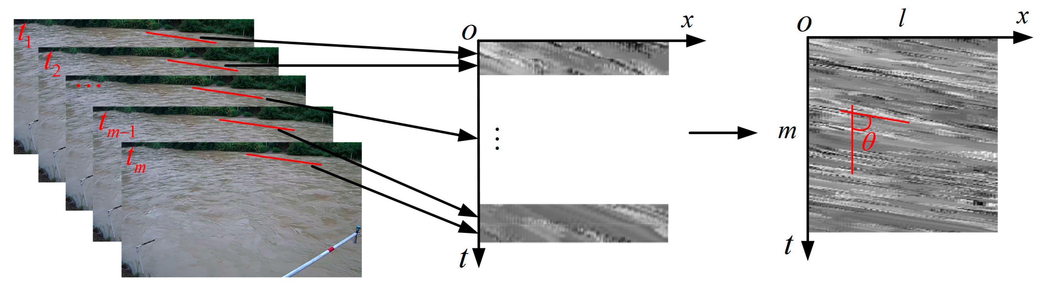
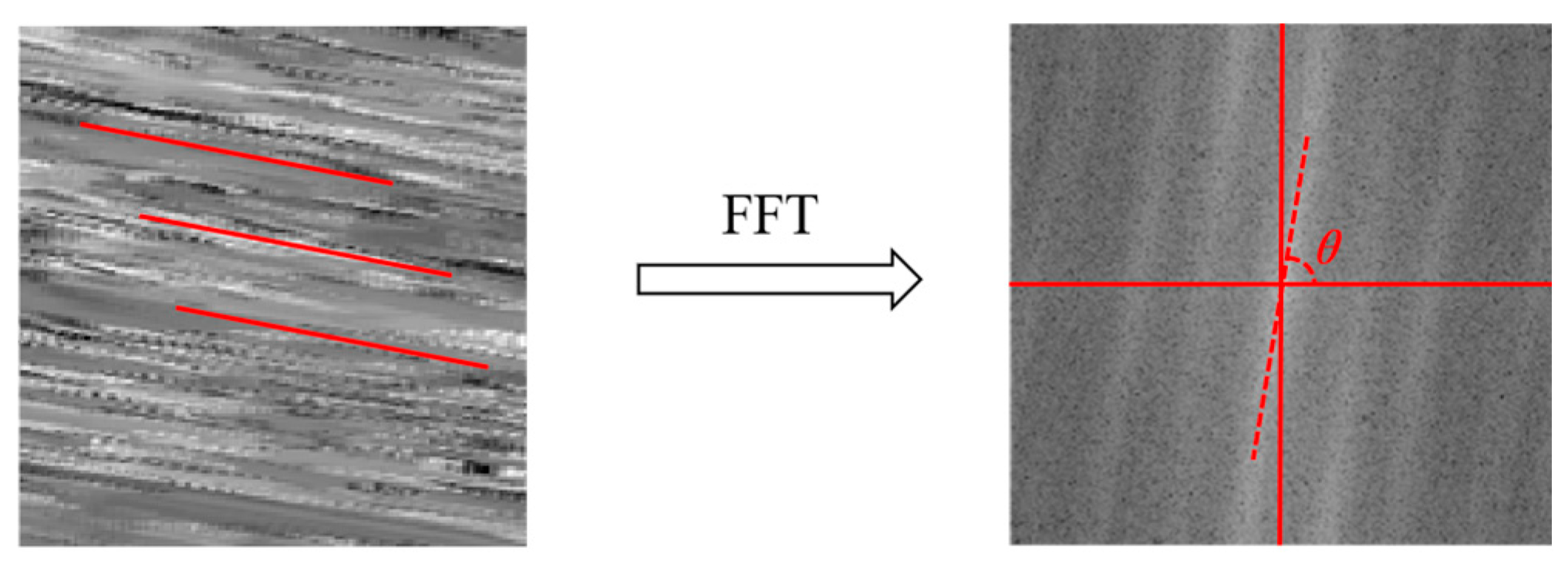
2.1. Generation of Space-Time Images

STIV is a non-contact measurement method that takes the velocimetry lines as the analysis area and estimates surface velocity by detecting the texture angle of the synthesized space-time images [18]. Firstly, a camera installed on the bank is used to collect an image sequence of m frames of the river surface in a certain time interval t ; then, a series of velocimetry lines are set along the direction of the actual movement of the water; these lines are only the width of a single pixel with a length of l pixels. Next, a space-time image (STI) with a size of l   ×   m pixels is synthesized in an x t rectangular coordinate system constructed from the motion distance and time. Figure 1 shows the generation of ST images; the black and white texture trajectory is displayed in the space-time image, and the angle θ between these texture trajectories and the vertical direction is defined as the main orientation of texture (MOT).
Suppose that in the physical coordinate system, the distance of the river surface flow feature moving along the velocimetry lines in time t is x , corresponding to l pixels moving within m frames in the image coordinate system; then, the river surface velocity V on the velocimetry lines is shown in Equation (1).
V = x t = l k x m k t = tan θ k x k t = tan θ k x f p s
where k x (m/pixel) represents the actual distance of each pixel, k t (s/pixel) represents the time interval between two frames, f p s (pixel/s) represents the camera frame rate, and t a n θ represents the tangent of the texture angle.

2.2. Construction of Datasets

The texture direction of the space-time images generated by the river video is chaotic, which is difficult to judge directly and accurately. Therefore, the ST images are converted into a frequency domain representation, as shown in Figure 2. The image feature extraction ability of deep convolutional neural network is utilized to obtain the mapping relationships from image space to angle space from a large number of training data, and then uses the learned relationship for angle prediction, which is a simple and efficient process with end-to-end implementation.
At present, the STIV method based on deep learning lacks publicly available image datasets of the river, so a high-definition video camera is installed at a fixed position on the bank of the hydrological station to record river flow videos at different time periods to construct the datasets. The common texture angle of the STIs is [5°, 85°]. Considering the difficulty of collecting river video in specific complex scenes and making the constructed dataset representative, four common scenes, including normal, exposure, turbulence, and blur conditions, are selected to generate STIs. Artificial spectrum labeling is adopted to label texture angle sizes, and unified integer as classification labels. The STIs generated under real river conditions contain a lot of noise, which may be completely treated as such datasets will make the model learn the noise patterns during training, and the angle values may be incorrectly detected, affecting the accuracy of the datasets. Therefore, some synthetic images created with Berlin noise are incorporated into the datasets, which are ideal STIs and have the characteristics of no noise interference and accurate known MOT values.
Since it is not possible to generate STIs for all angles, it is necessary to augment the original images to increase the diversity and variability of training data. The data augmentation process involves the following steps: the images are rotated in 1-degree steps with the center of the images as the origin to generate 81 classes of space-time images with a given texture angle, and then these images are transformed into frequency domain representation with an image size of 224 × 224 pixels for training. Figure 3 shows the images of the datasets in various scenarios randomly selected, and the sequence is normal, exposure, turbulence, blur, and synthesis. Table 1 displays the dataset’s distribution.

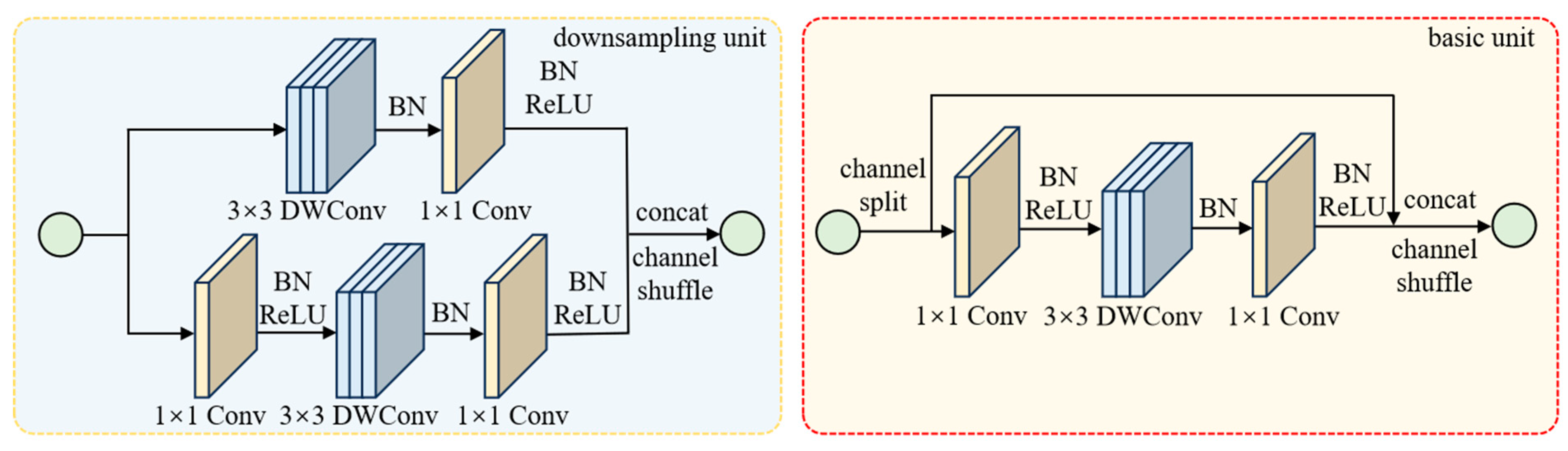
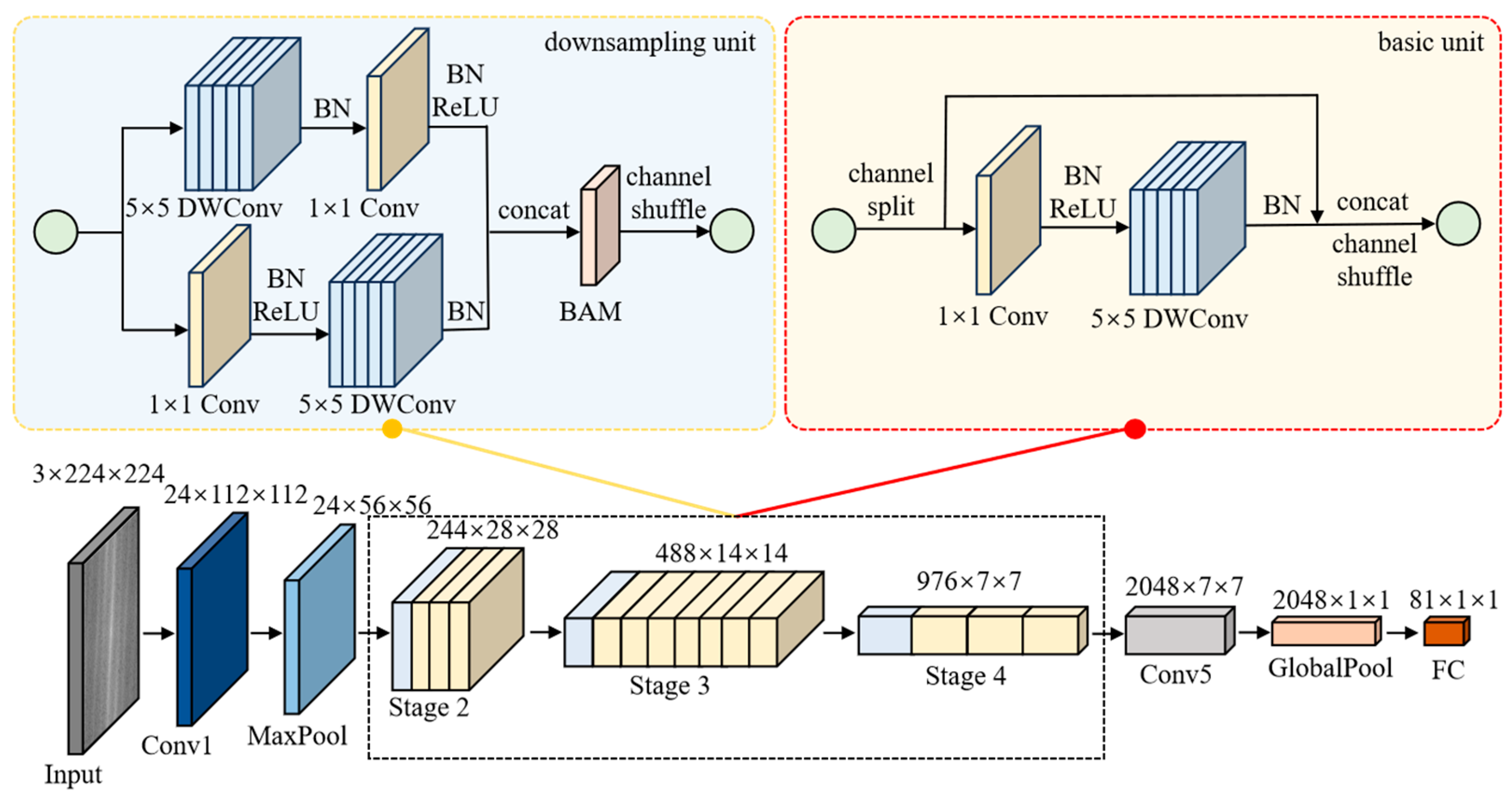
2.3. Structure of ShuffleNetV2

ShuffleNetV2 [19], introduced by Megvii Technology, is an efficient and lightweight convolutional neural network. ShuffleNetV2 retains the core operations from its predecessor ShuffleNetV1 [20], such as channel shuffle, group convolution, and depthwise separable convolution. Beyond that, ShuffleNetV2 takes into account the impact of Memory Access Cost (MAC) on the model performance on the basis of ShuffleNetV1, ensuring that the network architecture is optimized for speed. The overall design of the network adheres to four guidelines: keep the width of the input and output channels equal, employ group convolution appropriately, minimize the degree of network fragmentation, and reduce the element operations.
The basic structure of ShuffleNetV2 is depicted in Figure 4; it is mainly composed of a downsampling unit and a basic unit. The downsampling unit is designed with a stride of 2, which effectively halves the spatial dimensions of the input features. The feature maps are dually processed through two distinct branches. The main branch undergoes two 1 × 1 conventional convolutions, and employs a 3 × 3 depthwise separable convolution (DWConv) in the middle for feature extraction, while the other branch applies a conventional 1 × 1 convolution and a 3 × 3 depthwise separable convolution with a stride of 2. The final step involves concatenating the feature maps and performing a channel shuffling operation. In the basic unit with a stride of 1, the input feature map is divided into two branches by channel split. The main branch operates the same as the downsampling unit, while no operation is performed in the other branch. Ultimately, the channels from both branches are concatenated and a channel shuffling operation is carried out.

2.4. Improvement of ShuffleNetV2
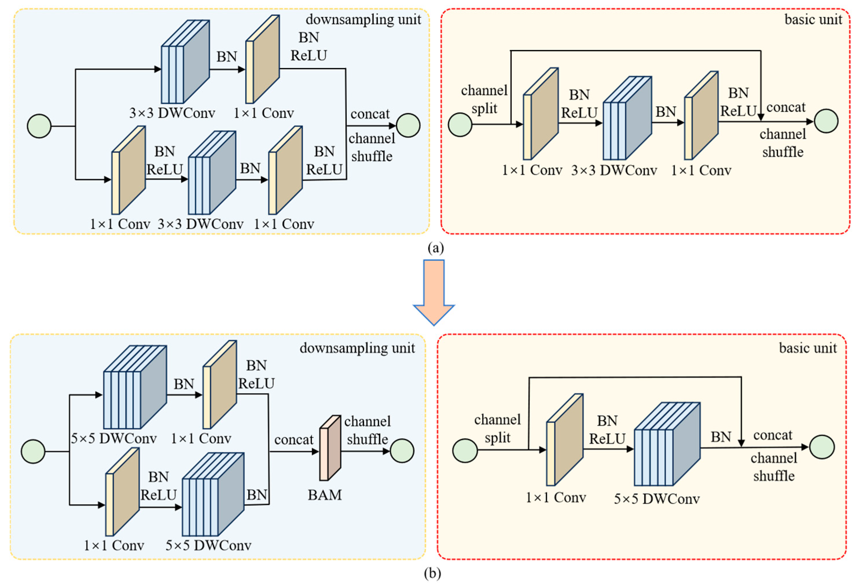
We take ShuffleNetV2_2.0 as the backbone network in this research and improve it. The overall structure of the improved network is shown in Figure 5. Firstly, the second 1 × 1 convolution in the main branch of both the downsampling unit and basic unit is deleted; secondly, the kernel size of all depthwise separable convolutions is increased from 3 × 3 to 5 × 5; additionally, the Bottleneck Attention Module (BAM) [21] is introduced, and it is added after the channel concatenation operation of the downsampling unit.

2.4.1. Delete the Second 1   ×   1 Convolution and Enlarge DWConv Kernel Size

Typically, there are two purposes for using 1 × 1 convolution before and after DWConv. One is to fuse inter-channel information to compensate for the limitations of DWConv, the other is to perform a dimensional adjustment, which may be a reduction or expansion in dimension. The ShuffleNetV2 network uses two 1 × 1 convolutions when fusing channel information, but this task can be accomplished with only one 1 × 1 convolution. Therefore, to delete the second 1 × 1 convolution in the main branch of downsampling unit and the basic unit can not only preserve the ability to fuse information, but also reduce the calculation amount of the model.
As can be seen from the distribution of the computational volume of ShuffleNetV2, the vast majority of the computational volume is concentrated on the 1 × 1 convolution, with DWConv contributing a relatively smaller portion. To improve the detection accuracy without significantly increasing the computational effort, we change the kernel size of all DWConv from 3 × 3 to 5 × 5. The padding needs to be adjusted from 1 to 2 to ensure that the dimension of the output feature maps remains constant in the PyTorch code.

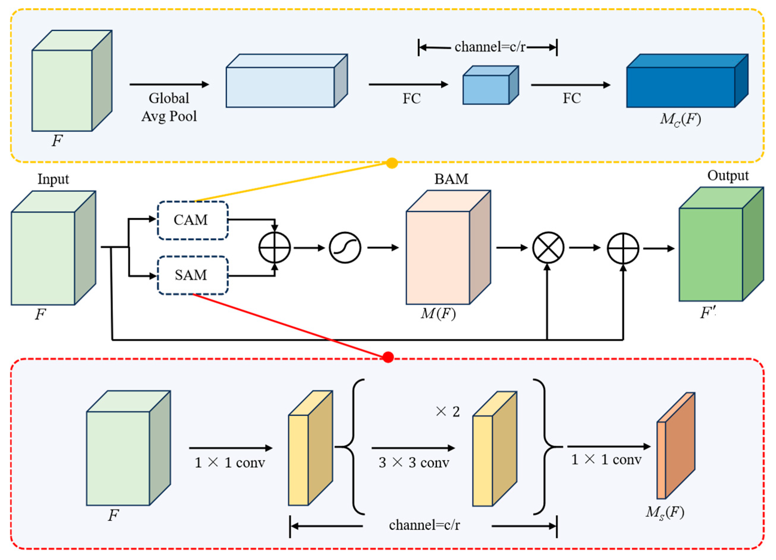
2.4.2. Bottleneck Attention Module (BAM)

In order to enable the neural network to learn the feature information in complex scenes and improve the accuracy of texture angle recognition, we integrate a BAM attention module after the channel concatenation in the downsampling unit, followed by a channel shuffling operation. BAM is a lightweight Bottleneck Attention Module, as shown in Figure 6, which consists of a Channel Attention Module (CAM) and a Spatial Attention Module (SAM).
Global average pooling is performed on the input feature map F to aggregate and enhance feature information in the CAM, and more channel attention is obtained through the shared Multilayer Perceptron, and then the global maximum pooling result of each channel is transmitted through the two fully-connected layers to generate channel attention features M C F . The calculation process is shown in Equation (2).
M C F = B N M L P A v g P o o l F
The SAM adopts a bottleneck structure similar to ResNet to emphasize or suppress features at different spatial locations. Firstly, the feature is projected onto the reduced dimension R c / r × H × W by 1 × 1 convolution, then two 3 × 3 dilation convolutions are used to effectively utilize the context information, and finally further dimensionality reduction by a 1 × 1 convolution obtains spatial attention features M S F with dimension R 1   ×   H   ×   W . The calculation process is shown in Equation (3).
M S F = B N f 3 1   ×   1 f 2 3   ×   3 f 1 3   ×   3 f 0 1   ×   1 F
M C F and M S F are added together and activated by the S i g m o i d activation function to generate 3D attention features M F , as shown in Equation (4). M F is multiplied by the input feature map F and then added to the input feature map F to obtain the final feature map F , as shown in Equation (5).
M F = σ M C F + M S F
F = F + F M F

2.5. Camera Calibration

After the texture angle of the space-time image is obtained, it is necessary to further utilize the principle of projection transformation to achieve the conversion between the world coordinate system and the pixel coordinate system, so as to obtain the actual distance represented by each pixel, which is denoted by k x . Having selected a calibration point on the riverbank as the origin of the world coordinate system, the line connecting this origin to another calibration point on the same horizontal plane is considered the x-axis direction, and the perpendicular line from the origin to the calibration point on the opposite bank is considered the y-axis direction. According to the positional relationship of the ground calibration points, the world coordinates of each calibration point are measured by a total station, and the pixel coordinates correspond one by one. Assuming a point ( i , j ) in the pixel coordinate system corresponds to the position ( x , y , z ) in the world coordinate system, the transformation relationship can be expressed as Equation (6), η m n ( m , n = 1 3 ) is the corresponding transmission transformation matrix.
x y z = η 11 η 12 η 13 η 21 η 22 η 23 η 31 η 32 η 33 i j 1
After expanding the equation, the final coordinate relationship is shown in Equation (7). Therefore, the position of the ground calibration points and the velocimetry points on the river section in the world coordinate system can be accurately marked in the pixel coordinate system.
x = η 11 i + η 12 j + η 13 η 31 i + η 32 j + η 33 y = η 21 i + η 22 j + η 23 η 31 i + η 32 j + η 33

2.6. Calculation of River Velocity and Discharge

After calculating the river surface velocity, the total discharge and mean velocity are calculated according to the velocity–area method. As shown in Figure 7, the arrow direction represents the flow of water. Suppose that the surface flow velocity of the measuring point i is V i , and the width between the measuring points i 1 and i is d i , and h i 1 and h i denote the actual water depth (m) corresponding to the vertical line of the measuring points i 1 and i , respectively, then the partial area S i 1 , i between the two measuring points is shown in Equation (8).
S i 1 , i = h i 1 + h i 2 d i
The vertical mean velocity V m i is shown in Equation (9), where μ denotes the surface velocity coefficient.
V m i = μ V i
The partial mean velocity V i 1 , i ¯ between the two measuring points is shown in Equation (10).
V i 1 , i ¯ = V m ( i 1 ) + V m i 2
The partial mean velocity near the bank is shown in Equations (11) and (12), where ε denotes velocity coefficient on the bank; its value usually follows the Chinese national measurement specifications standard GB 50179-2015 [22]. When on slopes where the water depth gradually becomes shallower to zero on banks, ε ranges from 0.67 to 0.75, and ε is 0.8 and 0.9 on the steep banks of an uneven riverbank and even riverbank and ε is 0.6 at the river bank or in a stagnant water area.
V 1 ¯ = V m 1 ε
V i ¯ = V m i ε
After calculating the partial mean velocity of each part, the product of it and the partial area is the discharge of each part, and then the total discharge Q is the sum of the discharge of all parts, as shown in Equation (13).
Q = i = 1 n V i ¯ S i
The mean velocity V ¯ is calculated according to the total discharge Q and the cross-section area S , as shown in Equation (14).
V ¯ = Q S = Q S 1 + i = 2 i S i 1 , i + S i

3. Results and Discussion

3.1. Model Training

The experimental hardware environment is an Intel (R) Core (TM) i7-6700K CPU @ 4.00 GHz and a NVIDIA GeForce RTX 2060 GPU with 6 GB of video memory; software environment is Windows 10 64 bit operating system, the program is run on Python 3.8, and the deep learning framework is PyTorch 1.9. The Adam optimizer is used to optimize the network backpropagation and the loss function is cross-entropy. The initial learning rate is 0.001, the number of training iterations is 200, and the batch size is 32.

3.2. Model Performance Comparison

TOP1 and TOP5 accuracy are chosen to evaluate the classification performance of the model in the experiment, and the number of parameters (Params) and FLOPs are selected to further evaluate the hardware requirements and the complexity of the model. TOP1 accuracy refers to the proportion where the category with the highest predicted probability by the model matches the true label. If the predicted category is consistent with the true label, the sample is considered to be correctly classified. TOP5 accuracy refers to the proportion where the true label appears among the top five categories with the predicted probabilities by the model; as long as the true label is within the top five predictions, the sample is considered to be correctly classified. The number of parameters is directly related to the size of the model and its demand for computing resources and storage. The number of calculations refers to the number of floating-point operations per second, which directly determines the run speed of the model. The greater the amount of computation, the longer the training time, and the higher the requirement of computing capabilities.
Comparative experiments are conducted using original ShuffleNetV2, improved ShuffleNetV2, and other networks to comprehensively evaluate the performance.

3.2.1. Comparison of ShuffleNetV2 Series Models

Similar to ShuffleNetV1, the number of channels in each block of the ShuffleNetV2 is scaled to create networks of different complexity, and denoted as ShuffleNetV2_0.5, ShuffleNetV2_1.0, ShuffleNetV2_1.5, and ShuffleNetV2_2.0. Among them, _0.5, _1.0, _1.5, and _2.0 are scaling factors which is related to the number of output channels in each layer of the network. Their experimental results on the datasets are illustrated in Table 2.
It can be seen from the data in the Table 2 that using the same experimental platform and hyperparameter settings, ShuffleNetV2_2.0 achieves a higher classification accuracy than the other three models, although the amount of parameters and FLOPs is relatively high. We choose to further improve ShuffleNetV2_2.0 after comprehensive considerations and conduct other related experiments based on the frequency domain image datasets.

3.2.2. Ablation Experiment

In order to facilitate the ablation experiments, we designed models 0 to 3. The basic structure of the module for model 0 is shown in Figure 8a, while the basic structure of the modules for models 1 to 3 is shown in Figure 8b.
Model 0 is the original ShuffleNetV2_2.0, model 1 only reduces the 1 × 1 convolution in the main branch of the downsampling unit and basic unit, model 2 enlarges the DWConv kernel from 3 × 3 to 5 × 5 based on model 1, and model 3 increases BAM attention based on model 2. The ablation experiments are conducted and the results are detailed in Table 3, where Lite_1 × 1 means to delete the 1 × 1 convolution operation, K_size = 5 means to change the DWConv kernel to 5 × 5, and “√” indicates that this operation is performed.
It is noticeable that the performance of the model is gradually improved with the addition of each improvement factor. To be specific, model 1 exhibits a reduction of 27.52% in the number of parameters and 34.92% in the number of FLOPs compared to model 0 and the accuracy of model 2 is increased by 2.97% and 0.81%, respectively, on the original basis. Model 3 integrates all the improvement factors, resulting in a significant improvement in performance. The TOP1 accuracy is increased by 5.99%, the TOP5 accuracy is improved by 0.75% over the original ShuffleNetV2_2.0, and the numbers of parameters and calculations are reduced by 20.14% and 34.92%, respectively. All in all, deleting 1 × 1 convolution, enlarging the DWConv kernel, and introducing BAM attention all significantly enhance the classification performance, proving that the improved methods are effective.
In addition, in order to further verify the superiority of the BAM attention mechanism in improving the model effect, a comparison experiment was conducted between BAM attention mechanism and the Efficient Channel Attention (ECA) [23], the Convolutional Block Attention Module (CBAM) [24], and the Squeeze-and-Excitation (SE) [25] attention mechanisms, and the experimental results are shown in Table 4.
The experimental results show that the addition of various attention mechanisms to model 2 has different effects on the classification performance. In particular, the BAM attention mechanism is the most effective. In contrast, the performance of ECA and CBAM attention in this experiment is not as good as that of the basic model, while the SE attention mechanism has some performance improvement, but the effect is still not as good as BAM. The BAM attention mechanism enhances the ability to extract different image features more effectively than other attention mechanisms, while ignoring those with less correlation. Although there is a slight increase in parameters and computation with the addition of BAM, the increase is worthwhile.

3.2.3. Comparison of Different Network Models

The comparative experiments are conducted with other networks ResNet34 [26], DenseNet [27], MobileNetV2 [28], EfficientNetV2 [29], and GhostNetV1 [30] on the same experimental platform to comprehensively evaluate the performance of the improved network. Care is taken to ensure that all relevant parameters remain constant to guarantee the fairness of the experiments. The experimental results of these various networks are presented in Table 5.
According to the data shown in Table 5, the TOP1 accuracy of the improved model reaches 64.69%, which is notably superior to that of the original model and other competing networks. Furthermore, the TOP5 accuracy stands at 90.56%, and it significantly outperforms ResNet34, DenseNet, and EfficientNetV2 in terms of parameters and FLOPs. When compared to MobileNetV2 and GhostNetV1, the improved model demonstrates a higher detection accuracy. This indicates that the improvements have been successful in boosting its accuracy without incurring excessive computational costs, and hence it exhibits a more favorable overall performance.

3.3. Experiments in the Measurement of River Velocity and Discharge

The texture angle of the STI is detected by image classification, and the surface velocity of each velocity point is calculated, and then the total discharge and mean velocity of the river are obtained. The results obtained from the current meter are usually considered as the true value and treated as a criterion for comparison with other methods in the measurement of river velocity and discharge. We have chosen vertical mean velocity, total discharge, and mean velocity as the key measurement indicators in this research. The river images are captured at a resolution of 1920 × 1080 in all experiments. During the same time period that the current meter is operating, comparative measurement experiments are carried out in an artificially repaired and two natural rivers, respectively, by using GTM [9], FFT [11], FD-DIS-G [31], and the proposed method. FD-DIS-G proposed by Wang et al. [31] combines the frame difference with fast optical flow estimation using Dense Inverse Search (DIS) [32], and generates a motion significance graph to capture the water surface motion features by calculating the difference between image frames, then uses the DIS algorithm to calculate the dense optical flow, and finally performs singular value processing on the obtained data by means of groupings. The errors associated with each method are then compared and analyzed to assess their accuracy and reliability.

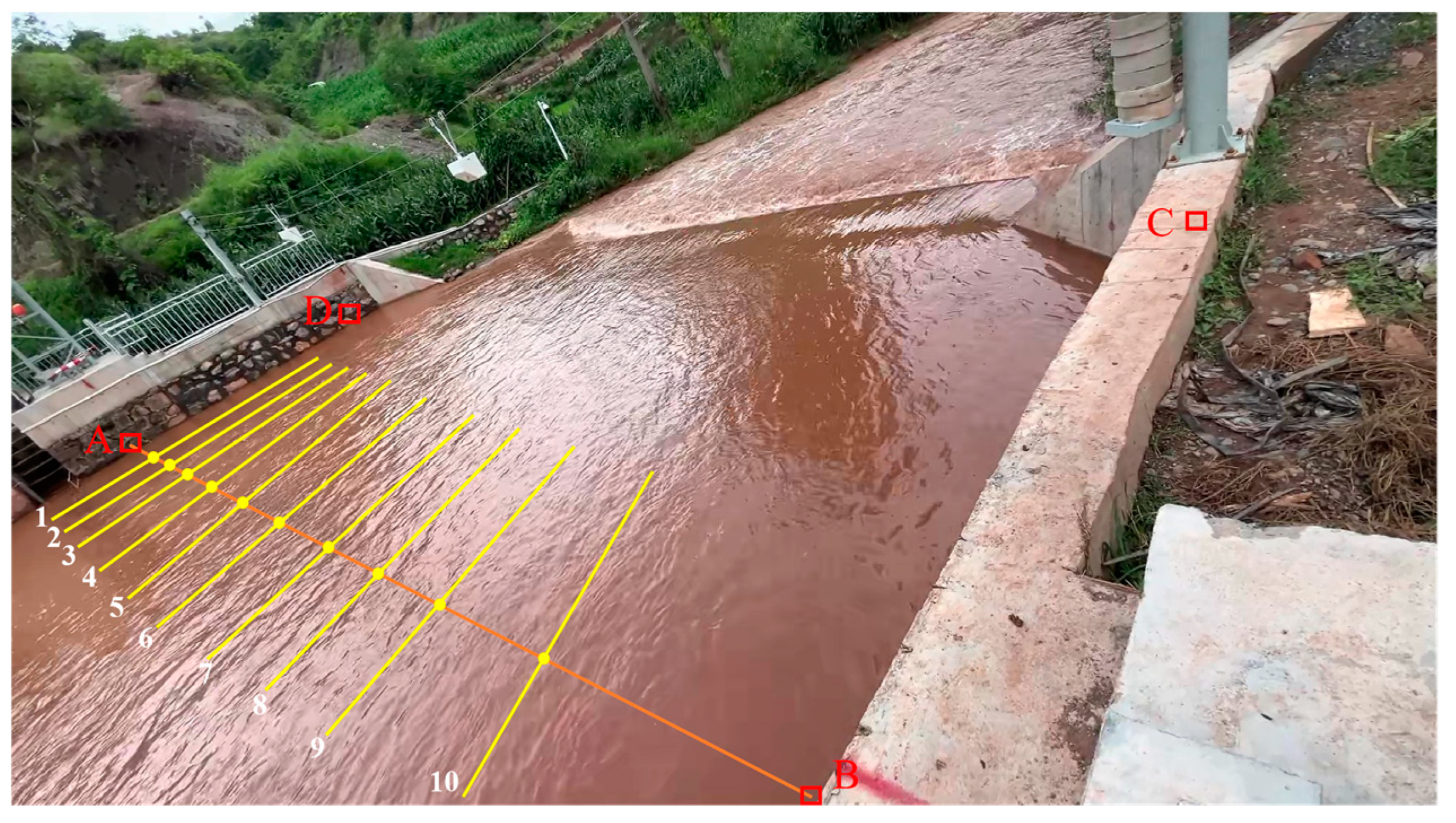
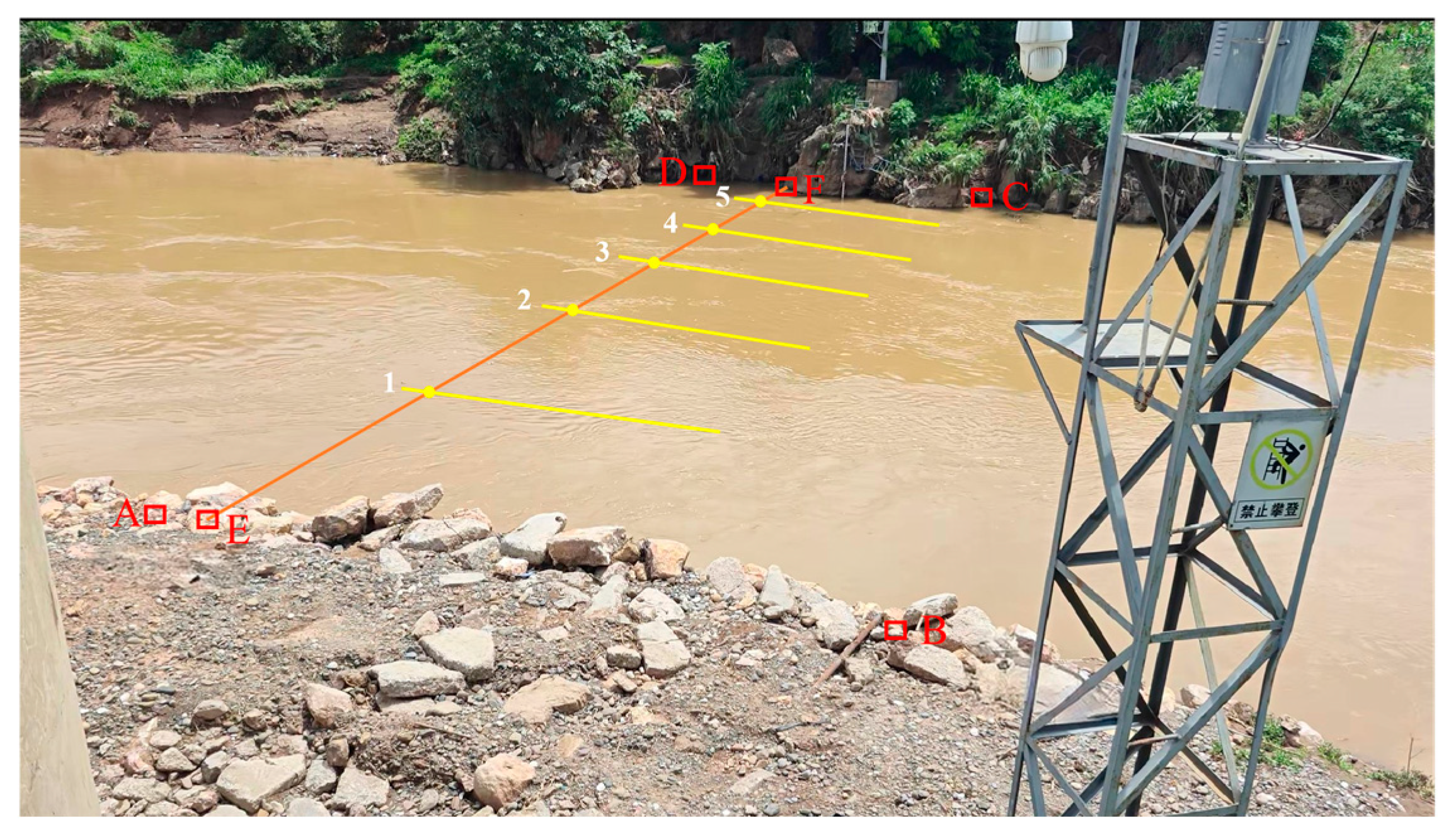
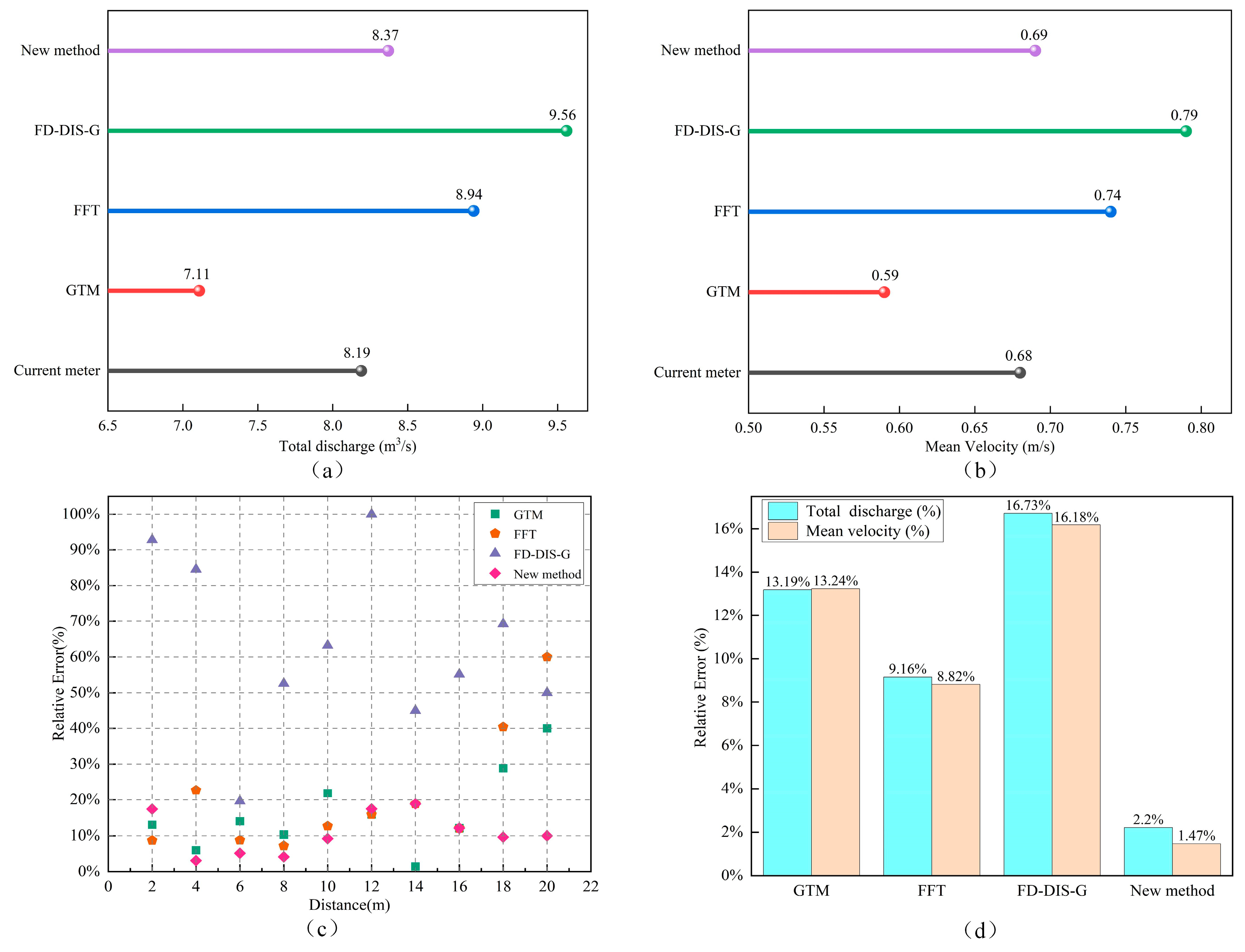
3.3.1. Experiment in an Artificially Repaired River

In order to verify the actual measurement effect of the proposed method, the Agu hydrology station located in Yimen County, Yuxi City, Yunnan Province is selected as the experimental site. Agu station has been artificially repaired, the river section is regular, and the velocity is stable. According to the annual measurement records of the hydrology station, the velocity coefficient on the bank is 0.75, and the surface velocity coefficient is 0.89. The camera view for capturing video is shown in Figure 9; the points A, B, C, and D, marked with red boxes, represent the location of the selected ground calibration points, and AB is the cross-section line. The velocimetry points represented by yellow solid points are set at distances of 2 m, 4 m, 6 m, 8 m, 10 m, 12 m, 14 m, 16 m, 18 m, and 20 m from point A, respectively, and are sequentially numbered from No. 1 to No. 10. The yellow lines are velocimetry lines laid at each measuring point.
A Hikvision DS-2DC7423 camera is fixed at distances of 24.2 m, 2.7 m, 8.5 m, 29.3 m from points A, B, C, and D, respectively, to record 5s of river video images, and the frame rate is 60 fps. Table 6 presents the cross-section data and values measured by the LS25-1 current meter. The results and errors derived from various methods are shown in Table 7. The intuitive comparison results and errors of vertical mean velocity, total discharge, and mean velocity are depicted in Figure 10.
The total discharge and mean velocity measured by the proposed method are 8.37 m3/s and 0.69 m/s, respectively. The absolute errors are 0.18 m3/s for discharge and 0.01 m/s for mean velocity, with relative errors of 2.20% and 1.47%, respectively. Compared with the GTM, FFT, and FD-DIS-G methods, the accuracy of discharge is increased by 10.99%, 6.96%, and 14.53%, and the accuracy of mean velocity is increased by 11.77%, 7.35%, and 14.71%, respectively, which indicates that the results of the new method are closest to the true value of the current meter and exhibits a high degree of consistency. For individual velocity measurement points, as shown in Figure 10c, the relative errors of the vertical mean velocity are maintained below 10% at points 2, 3, 4, 5, 9, and 10, and identical to those obtained by the FFT method at velocimetry points 7 and 8, and the relative errors are kept within the range of 12% to 19%, and the high accuracy of the measurements is still maintained even in the case of the most serious influence of the illumination, which confirms that it has good robustness and stability. In contrast, the GTM and FFT methods perform at a moderate level, while the measurement values and error fluctuations of FD-DIS-G are the largest, indicating that the stability is poor. The error of one velocimetry point is as high as 100%, which is attributed to the sensitivity to environmental noisy conditions of the FD-DIS-G method, and it can be clearly seen that the presence of a significant uneven illumination in the video of the river leads to a large measurement deviation of FD-DIS-G at each point. Its robustness needs to be improved.
Beyond that, the running time of the FD-DIS-G method is the shortest, only 32.75 s, followed by the BGT method (50.96 s) and the FFT method (67.03 s), while the time of the new proposed method is 115.43 s, which is much slower than the other methods. Deep Learning takes a long time to learn the data during the training phase, but after the training is completed, its advantage for improving precision is obvious, so the running efficiency of the proposed method can be ignored in actual measurement work.

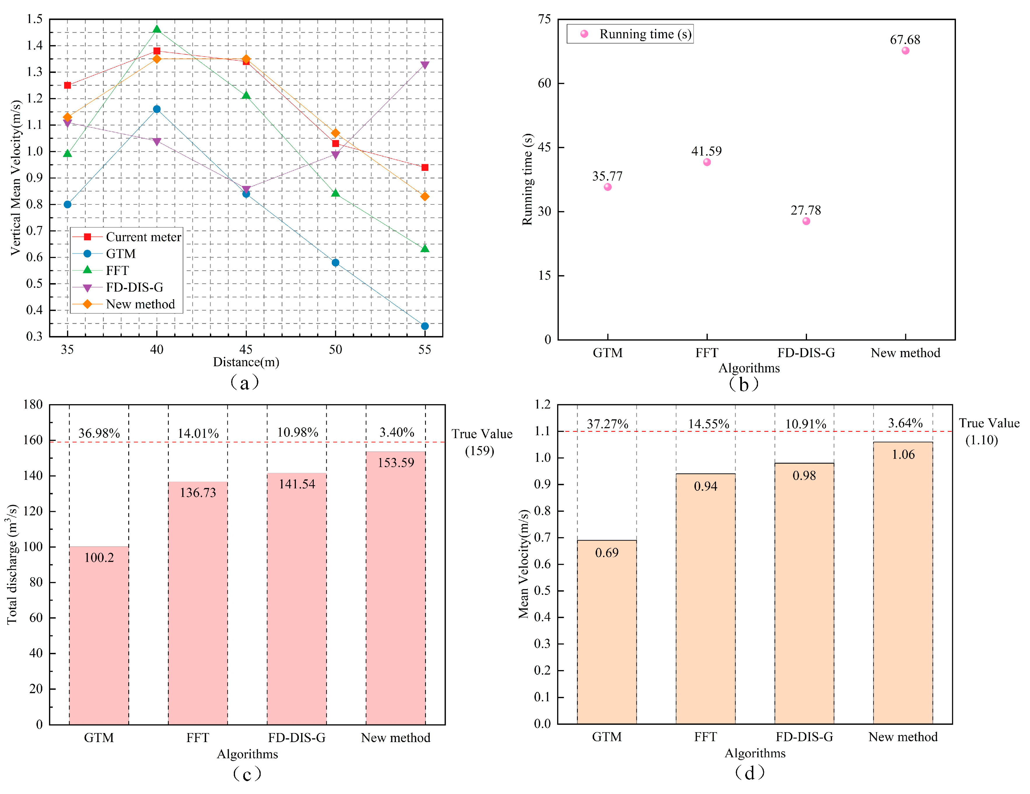
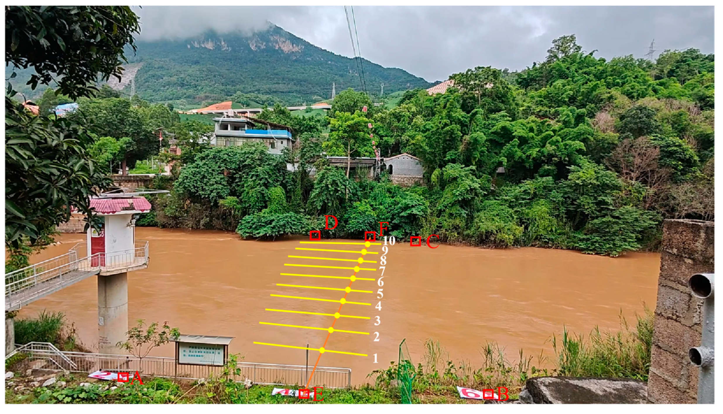
3.3.2. Experiment in Natural Rivers

To assess the applicability of the new proposed method in natural rivers, a verification experiment is conducted at Panxi hydrology station, located in Huaning County, Yuxi City, Yunnan Province, where the banks are irregular, there are many rocks at the bottom of the river, and vortices are generated in some areas of the water surface. According to the years of measurement experience of the hydrology station, the velocity coefficients of the left and right banks are 0.80 and 0.70, respectively, and the surface velocity coefficient is 0.88. As shown in Figure 11, the ground calibration points, marked with red boxes A, B, C, and D, are set on both sides of the river, and E to F is designed as the cross-section line; the five yellow solid points are velocimetry points, which are set at the distances 35 m, 40 m, 45 m, 50 m, 55 m away from point E, respectively, and named as No. 1 to No. 5 in turn. Furthermore, the yellow velocimetry lines are arranged at equal intervals along the direction of water flow.
A Hikvision DS-2DC1225-I3/I5 camera is used to record a 15 s river video at 25 frames per second from a location that is 13.1 m away from point A, 4.5 m away from point B, 36.4 m away from point C, and 44.8 m away from point D. Table 8 provides a detailed presentation of the cross-section data and the measurements recorded by the LS25-1 current meter. The measured results of the comparison experiments conducted by different methods at the same time period and the calculated errors compared with the true values of LS25-1 are presented in Table 9. Figure 12 displays the comparison of different methods.
It can be concluded from the experimental data that the discharge and mean velocity measured by the proposed method are 153.59 m3/s and 1.06 m/s, respectively. When compared to the true values of the current meter, the absolute and relative errors of discharge are 5.41 m3/s and 3.40%, and the absolute and relative errors of mean velocity are 0.04 m/s and 3.64%. The accuracy of these measurements surpasses that of the GTM, FFT, and FD-DIS-G methods. As depicted in Figure 12a, there is significant fluctuation in the measured values of the vertical flow velocity measured by GTM, FFT, and FD-DIS-G at each velocity measurement point, and the vertical mean velocity measured by the new method has a very high consistency with the measured results of the current meter, and the relative errors are within 12%, with a maximum error of 11.70%. At the middle three velocimetry points, the absolute errors of vertical mean velocity are 0.03 m/s, 0.01 m/s, and 0.04 m/s, with relative errors of 2.17%, 0.75%, and 3.88%, respectively. The error fluctuations are the most minimal, indicating an overall superior performance. However, the velocimetry points close to the banks are affected by the lens aberration of the camera equipment, which makes the errors relatively large and is not conducive to improving measurement accuracy. Nonetheless, even in these cases, the measurement errors are still lower than those of the other three methods.
Figure 12b clearly shows the time consumption of the four algorithms. Compared with the BGT, FFT, and FD-DIS-G methods, the running time of the new method is the longest. However, it can provide more reliable measurement results, and the increased time is completely acceptable in the monitoring work of hydrological stations.
The above two sets of experiments demonstrate that the proposed method is well-suited for monitoring river velocity and discharge in both artificial and natural rivers, and the reliable measurement results can be obtained in complex natural environments. Further research and verification are required to establish its applicability under other river conditions.
The wide universality of the proposed method is further confirmed at the Mengxing hydrological station in Lincang City, Yunnan province. The edge of the river bank is covered with vegetation and weeds, and there are standing signs and guardrails along the shore. During the measurement process, a DS-2DC1225-I3/I5 camera produced by Hikvision is installed at a location that is 39.4 m, 35.8 m, 80.3 m, and 85.6 m away from points A, B, C, and D, respectively. A 20 s river video is recorded at a frame rate of 25 frames per second to capture the flow characteristics in detail. The velocity coefficient of the bank is 0.70, and the surface velocity coefficient is 0.90. Figure 13 shows the layout of the ground calibration points A, B, C, and D, as well as the 10 velocity-measuring lines, and EF is regarded as the cross-section line; E is the starting point, while F is the end point. The measured points named as No. 1 to No. 10 in turn are positioned at intervals of 4 m, as shown in the yellow solid points in the figure. Table 10 presents the cross-section data and the true values obtained from the LS25-3A current meter at the velocimetry points. Table 11 provides a comparative analysis of the measured results and the errors associated with several methods, including the proposed one.
The measurement results of the proposed method have proven to be the most precise. Specifically, the measured total discharge is 86.11 m3/s with a relative error of 2.37%, which is 10.31% and 6.14% higher than that of GTM and FFT. In terms of mean velocity, the relative error of the proposed method is only 1.87%, which is 10.28% and 6.54% lower than that of other methods, respectively, and its stability and accuracy are improved to a great extent. It is noted that the error of vertical mean velocity at the last velocimetry point reaches 104.76%, which is because the point is far away from the lens, and the flow field near the bank is chaotic, resulting in the generated space-time images of the river having more noise components and less effective texture information, whereas the relative errors at the remaining measurement points are all controlled within 28%. Although the measured errors of the vertical mean velocity of the GTM and FFT methods are lower than those of the new proposed method at certain points, the overall measurement effect of these two methods is not ideal. The comprehensive analysis of three sets of experimental results indicates that the proposed method can realize reliable measurement and has good stability, and the development of this technology makes it possible for STIV technology to be more widely used and popularized in the monitoring of velocity.

4. Conclusions

A river velocity and discharge measurement method based on improved ShuffleNetV2 is proposed in this study. It utilizes image classification to detect the river texture angle without image processing, and enhances the ability to extract image information in complex river scenes by adjusting and optimizing the network structure and introducing the BAM attention mechanism, which effectively solves the problems of traditional STIV in complex noisy environments such as accuracy and robustness. The training experiment results of the improved ShuffleNetV2 on the dataset show that the TOP1 accuracy is 64.69%, and the TOP5 accuracy is 90.56%. The three sets of experiments indicate that the river discharge and mean velocity are the closest to the true values measured by the current meter. Specifically, the relative errors of the discharge and mean velocity in the Agu artificial river are 2.20% and 1.47%, respectively. In the Panxi and Mengxing natural rivers, the measured relative errors in discharge are 3.40% and 2.37%, respectively, and the measured relative errors in mean velocity are 3.64% and 1.87%, respectively. Compared with the existing BGT, FFT, and FD-DIS-G methods, the proposed method is more effective and stable and confirms the potential of deep learning technology in the hydrological field. It not only provides a new technical means, but also promotes the construction and development of intelligent hydrology.
However, the proposed method still has some limitations in practical application. Future research should focus on collecting more diversified river video image data to cover different geographical features and climatic conditions, expanding the scope and variety of datasets, and conducting validation experiments in more river environments to further improve the generalization ability and adaptability of the model. In addition, we have only researched rivers with turbid water and a flow rate of about 1 m/s. Further work can be attempted to apply this method to cases with faster flow rates or clearer water to verify the advantages of the method.

Author Contributions

Conceptualization, R.L. and J.W.; methodology, R.L.; validation, R.L., J.J. and J.W.; formal analysis, R.L.; investigation, R.L.; resources, D.H., N.L. and X.P.; writing—original draft preparation, R.L.; writing—review and editing, R.L.; visualization, R.L.; supervision, J.J. and J.W.; project administration, J.J. and J.W.; funding acquisition, J.W. All authors have read and agreed to the published version of the manuscript.

Funding

This research was supported by the National Natural Science Foundation of China (No. 62363017) and ‘Yunnan Xingdian Talents Support Plan’ Project (No. KKXY202203006).

Institutional Review Board Statement

Not applicable.

Informed Consent Statement

Not applicable.

Data Availability Statement

The data supporting the findings of this study can be found within the article.

Conflicts of Interest

The authors declare no conflicts of interest.

References

  1. Ju, Z. Research on River Velocity Measurement Based on Video and Image Recognition. Master’s Thesis, Zhejiang University of Technology, Hangzhou, China, 2018. [Google Scholar]
  2. Kimiaghalam, N.; Goharrokhi, M.; Clark, S.P. Assessment of wide river characteristics using an acoustic Doppler current profiler. J. Hydrol. Eng. 2016, 21, 06016012. [Google Scholar] [CrossRef]
  3. Xu, L.; Zhang, Z.; Yan, X.; Wang, H.; Wang, X. Advances of Non-contact Instruments and Techniques for Open-channel Flow Measurements. Water Resour. Inform. 2013, 3, 37–44. [Google Scholar]
  4. Yang, D.; Shao, G.; Hu, W.; Liu, G.; Liang, J.; Wang, H.; Xu, C. Review of image-based river surface velocimetry research. J. Zhejiang Univ. Sci. 2021, 55, 1752–1763. [Google Scholar]
  5. Adrian, R.J. Scattering particle characteristics and their effect on pulsed laser measurements of fluid flow: Speckle velocimetry vs particle image velocimetry. Appl. Opt. 1984, 23, 1690–1691. [Google Scholar] [CrossRef] [PubMed]
  6. Fujita, I.; Muste, M.; Kruger, A. Large-scale particle image velocimetry for flow analysis in hydraulic engineering applications. J. Hydraul. Res. 1998, 36, 397–414. [Google Scholar] [CrossRef]
  7. Khalid, M.; Pénard, L.; Mémin, E. Optical flow for image-based river velocity estimation. Flow Meas. Instrum. 2019, 65, 110–121. [Google Scholar] [CrossRef]
  8. Fujita, I.; Tsubaki, R. A Novel Free-Surface Velocity Measurement Method Using Spatio-Temporal Images. In Proceedings of the 2002 Hydraulic Measurements and Experimental Method Specialty Conference, Estes Park, CO, USA, 28 July–1 August 2002; pp. 1–7. [Google Scholar]
  9. Fujita, I.; Watanabe, H.; Tsubaki, R. Development of a non-intrusive and efficient flow monitoring technique: The space-time image Velocimetry (STIV). Int. J. River Basin Manag. 2007, 5, 105–114. [Google Scholar] [CrossRef]
  10. Fujita, I.; Notoya, Y.; Tani, K.; Tateguchi, S. Efficient and accurate estimation of water surface velocity in STIV. Environ. Fluid Mech. 2019, 19, 1363–1378. [Google Scholar] [CrossRef]
  11. Zhen, Z.; Huabao, L.; Yang, Z.; Jian, H. Design and evaluation of an FFT-based space-time image velocimetry (STIV) for time-averaged velocity measurement. In Proceedings of the 2019 14th IEEE International Conference on Electronic Measurement & Instruments, Changsha, China, 1–3 November 2019; pp. 503–514. [Google Scholar]
  12. Zhao, H.; Chen, H.; Liu, B.; Liu, W.; Xu, C.Y.; Guo, S.; Wang, J. An improvement of the Space-Time Image Velocimetry combined with a new denoising method for estimating river discharge. Flow Meas. Instrum. 2021, 77, 101864. [Google Scholar] [CrossRef]
  13. Lu, J.; Yang, X.; Wang, J. Velocity Vector Estimation of Two-Dimensional Flow Field Based on STIV. Sensors 2023, 23, 955. [Google Scholar] [CrossRef] [PubMed]
  14. Yuan, Y.; Che, G.; Wang, C.; Yang, X.; Wang, J. River video flow measurement algorithm with space-time image fusion of object tracking and statistical characteristics. Meas. Sci. Technol. 2024, 35, 055301. [Google Scholar] [CrossRef]
  15. Watanabe, K.; Fujita, I.; Iguchi, M.; Hasegawa, M. Improving Accuracy and Robustness of Space-Time Image Velocimetry (STIV) with Deep Learning. Water 2021, 13, 2079. [Google Scholar] [CrossRef]
  16. Li, H.; Zhang, Z.; Chen, L.; Meng, J.; Sun, Y.; Cui, W. Surface space-time image velocimetry of river based on residual network. J. Hohai Univ. 2023, 51, 118–128. [Google Scholar]
  17. Huang, Y.; Chen, H.; Huang, K.; Chen, M.; Wang, J.; Liu, B. Optimization of Space-Time image velocimetry based on deep residual learning. Measurement 2024, 232, 114688. [Google Scholar] [CrossRef]
  18. Zhang, Z.; Li, H.; Yuan, Z.; Dong, R.; Wang, J. Sensitivity analysis of image filter for space-time image velocimetry in frequency domain. Chin. J. Sci. Instrum. 2022, 43, 43–53. [Google Scholar]
  19. Ma, N.; Zhang, X.; Zheng, H.T.; Sun, J. ShuffleNetV2: Practical Guidelines for Efficient CNN Architecture Design. In Proceedings of the 15th European Conference on Computer Vision, Munich, Germany, 8–14 September 2018; pp. 122–138. [Google Scholar]
  20. Zhang, X.; Zhou, X.; Lin, M.; Sun, J. ShuffleNet: An Extremely Efficient Convolutional Neural Network for Mobile Devices. In Proceedings of the 2018 IEEE/CVF Conference on Computer Vision and Pattern Recognition, Salt Lake City, UT, USA, 18–23 June 2018; pp. 6848–6856. [Google Scholar]
  21. Park, J.; Woo, S.; Lee, J.Y.; Kweon, I.S. Bam: Bottleneck Attention Module. arXiv 2018, arXiv:1807.06514. [Google Scholar]
  22. GB 50179-2015; Code for Liquid Flow Measurement in Open Channels. Beijing China Planning Publishing House: Beijing, China, 2015. (In Chinese)
  23. Wang, Q.; Wu, B.; Zhu, P.; Li, P.; Zuo, W.; Hu, Q. ECA-Net: Efficient channel attention for deep convolutional neural networks. In Proceedings of the 2020 IEEE/CVF Conference on Computer Vision and Pattern Recognition, Seattle, WA, USA, 13–19 June 2020; pp. 11534–11542. [Google Scholar]
  24. Woo, S.; Park, J.; Lee, J.Y.; Kweon, I.S. Cbam: Convolutional block attention module. In Proceedings of the 15th European Conference on Computer Vision (ECCV), Munich, Germany, 8–14 September 2018; pp. 3–19. [Google Scholar]
  25. Hu, J.; Shen, L.; Sun, G. Squeeze-and-excitation networks. In Proceedings of the IEEE Conference on Computer Vision and Pattern Recognition, Salt Lake City, UT, USA, 18–23 June 2018; pp. 7132–7141. [Google Scholar]
  26. He, K.; Zhang, X.; Ren, S.; Sun, J. Deep residual learning for image recognition. In Proceedings of the 2016 IEEE Conference on Computer Vision and Pattern Recognition, Las Vegas, NV, USA, 27–30 June 2016; pp. 770–778. [Google Scholar]
  27. Huang, G.; Liu, Z.; Van Der Maaten, L.; Weinberger, K.Q. Densely connected convolutional networks. In Proceedings of the 2017 IEEE Conference on Computer Vision and Pattern Recognition, Honolulu, HI, USA, 21–26 July 2017; pp. 4700–4708. [Google Scholar]
  28. Sandler, M.; Howard, A.; Zhu, M.; Zhmoginov, A.; Chen, L.C. Mobilenetv2: Inverted residuals and linear bottlenecks. In Proceedings of the 2018 IEEE/CVF Conference on Computer Vision and Pattern Recognition, Salt Lake City, UT, USA, 18–23 June 2018; pp. 4510–4520. [Google Scholar]
  29. Tan, M.; Le, Q. Efficientnetv2: Smaller models and faster training. In Proceedings of the 38th International Conference on Machine Learning, PMLR, Virtual, 18–24 July 2021; pp. 10096–10106. [Google Scholar]
  30. Han, K.; Wang, Y.; Tian, Q.; Guo, J.; Xu, C.; Xu, C. Ghostnet: More features from cheap operations. In Proceedings of the 2020 IEEE/CVF Conference on Computer Vision and Pattern Recognition, Seattle, WA, USA, 13–19 June 2020; pp. 1580–1589. [Google Scholar]
  31. Wang, J.; Zhu, R.; Zhang, G.; He, X.; Cai, R. Image Flow Measurement Based on the Combination of Frame Difference and Fast and Dense Optical Flow. Adv. Eng. Sci. 2022, 54, 195–207. [Google Scholar]
  32. Kroeger, T.; Timofte, R.; Dai, D.; Van Gool, L. Fast optical flow using dense inverse search. In Proceedings of the 14th European Conference on Computer Vision, Amsterdam, The Netherlands, 11–14 October 2016; pp. 471–488. [Google Scholar]
Figure 1. Schematic diagram of space-time image synthesis.
Applsci 15 04865 g001
Figure 2. The process of FFT.
Applsci 15 04865 g002
Figure 3. Dataset images of different types.
Applsci 15 04865 g003
Figure 4. Basic structure of ShuffleNetV2.
Applsci 15 04865 g004
Figure 5. Overall structure of the improved ShuffleNetV2_2.0.
Applsci 15 04865 g005
Figure 6. BAM attention module.
Applsci 15 04865 g006
Figure 7. Schematic diagram of river cross-section.
Applsci 15 04865 g007
Figure 8. Module structure improvement of ShuffleNetV2_2.0. (a) Module structure of model 0; (b) module structure of models 1 to 3.
Applsci 15 04865 g008
Figure 9. Ground calibration points and velocimetry lines in Agu.
Applsci 15 04865 g009
Figure 11. Ground calibration points and velocimetry lines in Panxi.
Applsci 15 04865 g011
Figure 10. The results and analysis of different methods. (a) Results of the total discharge; (b) results of the mean velocity; (c) errors of the vertical mean velocity; (d) errors of the total discharge and mean velocity.
Applsci 15 04865 g010
Figure 12. The results and analysis of different methods. (a) Results of the vertical mean velocity; (b) comparison of running time; (c) results and errors of total discharge; (d) results and errors of mean velocity.
Applsci 15 04865 g012
Figure 13. Ground calibration points and velocimetry lines in Mengxing.
Applsci 15 04865 g013
Table 1. Dataset distributions.
TypeImage ClassTotal
NormalExposureTurbulenceBlurSynthetic
Train set/sheet810810810162040508100
Test set/sheet1621621623248101620
Total/sheet972972972194448609720
Table 2. Experimental results of ShuffleNetV2 series.
ModelTOP1/%TOP5/%Params/MFLOPs/G
ShuffleNetV2_0.551.3685.120.430.04
ShuffleNetV2_1.053.0985.861.350.16
ShuffleNetV2_1.555.6287.102.590.32
ShuffleNetV2_2.058.7089.815.560.63
Table 3. Ablation experiment results of ShuffleNetV2_2.0.
ModelLite_1 × 1K_Size = 5BAMTOP1/%TOP5/%Param/MFLOPs/G
0 58.7089.815.560.63
1 60.7490.934.030.41
2 61.6790.624.110.43
364.6990.564.440.45
Table 4. Effects of different attention mechanisms on model performance.
Attention MechanismTOP1/%TOP5/%Params/MFLOPs/G
-61.6790.624.110.43
ECA60.7489.514.110.43
CBAM61.1788.644.420.43
SE62.5388.954.270.43
BAM64.6990.564.440.45
Table 5. Comparison of experimental results of different networks.
ModelTOP1/%TOP5/%Param/MFLOPs/G
ResNet3464.1490.7421.373.68
DenseNet62.3590.007.042.90
MobileNetV258.4089.262.330.33
EfficientNetV262.5390.8620.282.90
GhostNetV158.2187.354.010.15
ShuffleNetV258.7089.815.560.63
Improved64.6990.564.440.45
Table 6. Data of cross-section and the LS25-1 current meter in Agu.
PointsStarting
Distance/(m)
Depth/(m)Vertical Mean Velocity/(m/s)Partial Mean Velocity/(m/s)Partial Area/(m2)Partial
Discharge/(m3/s)
0 (shore)
0–2 0.521.220.59
No. 120.540.69
2–4 0.831.010.84
No. 240.480.97
4–6 0.970.960.93
No. 360.480.97
6–8 0.970.990.96
No. 480.510.97
8–10 0.921.020.94
No. 5100.530.87
10–12 0.751.180.89
No. 6120.600.63
12–14 0.661.280.85
No. 7140.610.69
14–16 0.641.160.74
No. 8160.530.58
16–18 0.551.050.58
No. 9180.480.52
18–20 0.461.010.47
No. 10200.520.40
20–23 0.301.240.37
23 (shore)
Cross–section area/(m2): 12.12
Discharge/(m3/s): 8.19
Mean velocity/(m/s): 0.68
Table 7. Comparison of measured results and errors of different methods in Agu.
IndicatorsPointsMeasured Values/(m/s)Relative Error/(%)
Current MeterGTMFFTFD-
DIS-G
New MethodGTMFFTFD-
DIS-G
New Method
Vertical mean velocity /(m/s)No. 10.690.600.750.050.8113.04%8.70%92.75%17.39%
No. 20.970.911.190.151.006.19%22.68%84.54%3.09%
No. 30.970.831.060.781.0214.43%8.80%19.59%5.15%
No. 40.970.871.041.480.9310.31%7.22%52.58%4.12%
No. 50.870.680.981.420.9521.84%12.64%63.22%9.20%
No. 60.630.530.531.260.7415.87%15.87%100.00%17.46%
No. 70.690.680.561.000.561.45%18.84%44.93%18.84%
No. 80.580.650.510.900.5112.07%12.07%55.17%12.07%
No. 90.520.370.730.880.4728.85%40.38%69.23%9.62%
No. 100.400.240.640.600.4440.00%60.00%50.00%10.00%
Discharge/(m3/s)8.197.118.949.568.3713.19%9.16%16.73%2.20%
Mean velocity/(m/s)0.680.590.740.790.6913.24%8.82%16.18%1.47%
Table 8. Data of cross-section and the LS25-1 current meter in Panxi.
PointsStarting
Distance/(m)
Depth/(m)Vertical Mean Velocity/(m/s)Partial Mean Velocity/(m/s)Partial Area/(m2)Partial
Discharge/(m3/s)
23.6 (shore)
30–35 0.8832.828.9
No. 1354.461.25
35–40 1.3223.931.5
No. 2405.101.38
40–45 1.3625.034.0
No. 3454.971.34
45–50 1.1825.530.1
No. 4505.301.03
50–55 0.9827.527.0
No. 5555.700.94
55–57 0.7510.47.80
57 (shore)
Cross-section area/(m2): 145.00
Discharge/(m3/s): 159.00
Mean velocity/(m/s): 1.10
Table 9. Comparison of measured results and errors of different methods in Panxi.
IndicatorsPointsMeasured Values/(m/s)Relative Error/(%)
Current MeterGTMFFTFD-
DIS-G
New MethodGTMFFTFD-
DIS-G
New Method
Vertical mean
velocity/(m/s)
No. 11.250.800.991.111.1336.00%20.80%11.20%9.60%
No. 21.381.161.461.041.3515.94%5.80%24.64%2.17%
No. 31.340.841.210.861.3537.31%9.70%35.82%0.75%
No. 41.030.580.840.991.0743.69%18.45%3.88%3.88%
No. 50.940.340.631.330.8363.83%32.98%41.49%11.70%
Discharge/(m3/s)159.00100.20136.73141.54153.5936.98%14.01%10.98%3.40%
Mean velocity/(m/s)1.100.690.940.981.0637.27%14.55%10.91%3.64%
Table 10. Data of cross-section and the LS25-3A current meter.
PointsStarting
Distance/(m)
Depth/(m)Vertical Mean Velocity/(m/s)Partial Mean Velocity/(m/s)Partial Area/(m2)Partial
Discharge/(m3/s)
18.1 (shore)
21–24 0.327.132.28
No. 1242.020.45
24–28 0.707.725.40
No. 2281.860.96
28–32 1.127.848.78
No. 3322.081.28
32–36 1.348.0410.80
No. 4361.941.40
36–40 1.397.6010.60
No. 5401.861.38
40–44 1.387.3610.20
No. 6441.811.38
44–48 1.367.249.85
No. 7481.811.35
48–52 1.387.3610.20
No. 8521.881.40
52–56 1.307.7610.10
No. 9562.011.21
56–60 0.927.687.07
No. 10601.840.63
60–63 0.446.632.92
64.5 (shore)
Cross-section area/(m2): 82.40
Discharge/(m3/s): 88.20
Mean velocity/(m/s): 1.07
Table 11. Comparison of measured results and errors of different methods in Mengxing.
IndicatorsPointsMeasured Values/(m/s)Relative Error
Current MeterGTMFFTNew MethodGTMFFTNew Method
Vertical mean velocity/(m/s)No. 10.450.210.240.5553.33%46.66%22.22%
No. 20.961.201.230.7025.00%28.13%27.08%
No. 31.280.881.250.9731.25%2.34%24.22%
No. 41.400.851.231.1339.29%12.14%19.29%
No. 51.380.781.201.2143.48%13.04%12.32%
No. 61.381.461.221.235.80%11.59%10.87%
No. 71.352.041.221.2251.11%9.63%9.63%
No. 81.401.051.321.3725.00%5.71%2.14%
No. 91.211.231.081.431.65%10.74%18.18%
No. 100.630.420.521.2933.33%17.46%104.76%
Discharge/(m3/s)88.2077.0280.6986.1112.68%8.51%2.37%
Mean velocity/(m/s)1.070.940.981.0512.15%8.41%1.87%
Disclaimer/Publisher’s Note: The statements, opinions and data contained in all publications are solely those of the individual author(s) and contributor(s) and not of MDPI and/or the editor(s). MDPI and/or the editor(s) disclaim responsibility for any injury to people or property resulting from any ideas, methods, instructions or products referred to in the content.

