A Preference Model-Based Surrogate-Assisted Constrained Multi-Objective Evolutionary Algorithm for Expensively Constrained Multi-Objective Problems

Abstract

In the context of expensive constraint multi-objective problems, it is evident that the feasible domain shapes and sizes of different problems vary considerably. The difficulty in finding optimal solutions presents a significant challenge in ensuring the surrogate-assisted evolutionary algorithm’s feasibility, convergence, and diversity. To more effectively address the distinctive characteristics of the feasible domain and objective function across a range of problems, we have developed a Kriging-based surrogate-assisted evolutionary algorithm tailored to the current population’s preferences. The algorithm can optimize the population according to the current population’s requirements. Additionally, considering the varying degrees of accuracy observed in the surrogate models at different stages, this paper employs a dynamic approach to the number of surrogate model evaluations, contingent on the accuracy of the current surrogate model. Two types of Pareto frontier search are distinguished: unconstrained and constrained. Moreover, distinct fill sampling strategies are devised in accordance with the specific optimization requirements of the current population. After assessing the proposed solutions, the discrepancy between the actual fitness value and the surrogate model’s prediction is calculated.The discrepancy is used to modify the number of evaluations conducted on the surrogate model. In order to illustrate the algorithm’s efficacy, it is benchmarked against the current state-of-the-art algorithms on various test problems. The experimental results demonstrate that the proposed algorithm performs better than other advanced methods.

1. Introduction

Real-world engineering optimization problems often involve many conflicting objectives and some constraints [1]. A constrained multi-objective optimization problem (CMOP) with inequality constraints can be expressed as:

$$\begin{array}{cc}\hfill & \mathrm{minimize}F\left(x\right)={\left(f_1\left(x\right),\dots ,f_m\left(x\right)\right)}^T,\hfill \\ \hfill & \mathrm{s}.\mathrm{t}.g_j\left(x\right)\le 0,j\in \{1,2,\dots ,n\},\hfill \\ \hfill & x\in {\mathbb{R}}^d\hfill \end{array}$$

(1)

where $x={\left[\begin{array}{c}{x}_1,x_2,\dots ,x_D\end{array}\right]}^T$ is a d-dimensional decision variable, $f_1\left(x\right),\dots ,f_m\left(x\right)$ is the objective function to be optimized, and $g_j\left(x\right)$ is the first $\mathfrak{j}$ inequality constraint. For CMOP, constraint violation (CV) can be computed in the following way:

$$\mathrm{CV}\left(x\right)=\sum _{j=1}^{n}max(0,g_j\left(x\right))$$

(2)

A feasible solution refers to a solution whose CV value is less than or equal to 0. When a solution $x^{\ast }$ outperforms solution x on all objectives, $x^{\ast }$ dominates x. If $x^{\ast }$ is not dominated by other solutions, $x^{\ast }$ is called a non-dominated solution. The set of objective vectors formed by non-dominated solutions is called the constrained Pareto front. The goal of CMOP is to find the constrained Pareto front (CPF). There are a large number of constrained multi-objective problems in engineering problems in the real world. Some of these problems require expensive computational costs when being solved, such as fuel cell vehicle design [2], wire manufacturing [3], and space system design [4]. These types of problem are called expensive constrained multi-objective problems.

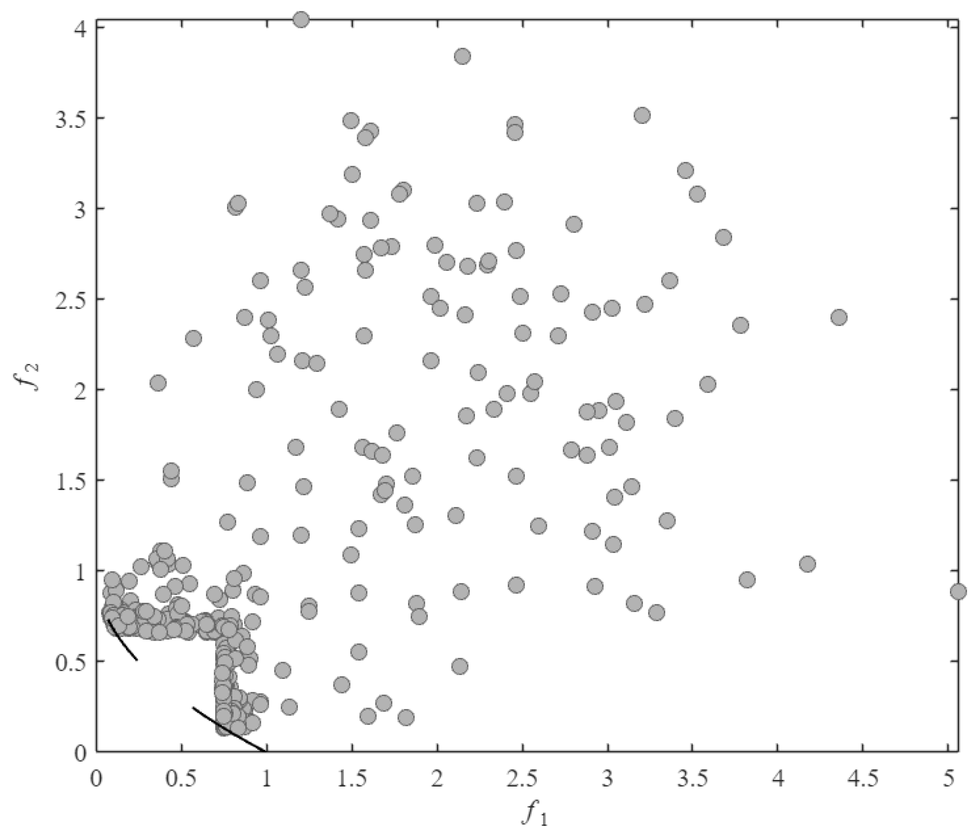
The ECMOP requires the algorithm to find the optimal solution under limited computational resources. However, the feasible domain is extremely narrow in MW1, which makes it difficult for the algorithm to find the feasible domain quickly. Meanwhile, the feasible domain of the problem is very broad for CF1 if the computational resources are heavily used in the constraint-value dominated search process, and the algorithm often falls into local convergence, making it difficult to approach the Pareto frontier. Therefore, the algorithm must use different search strategies for different feasible domains under different feasible domain conditions. In the case that the feasible domain is narrow and difficult to find, the algorithm needs to find the feasible domain with as few evaluations as possible, and in the case that there are already enough individuals in the feasible domain, it will not obtain good results if it pays too much attention to the convergence and feasibility. However, due to the limitation of computational resources, it is difficult for the algorithm to search for the optimal solution in a large decision space, requiring the algorithm to converge quickly to find the feasible domain. On the other hand, the complexity of CPF makes it difficult to explore the feasible domain with a limited number of solutions, which requires the algorithm to have good diversity.

Evolutionary algorithms are widely used in constrained multi-objective problems due to their advantages, such as simple implementation and strong search ability [5]. Constrained multi-objective evolutionary algorithms require using a large number of function evaluations to search the objective space to ensure the good performance of the algorithm. However, for ECMOPs, where the number of available function evaluations is limited, traditional constrained multi-objective evolutionary algorithms are not adept at generating solutions that meet the requirements [6].

In order to solve such problems, many researchers have used surrogate models instead of real evaluation functions to produce suitable solutions within a limited number of evaluations; this method is called surrogate-assisted MOEAs (SA-MOEAs). SA-MOEAs have become a promising direction in recent years [7] that has received increasing attention. Commonly used surrogate models in recent years include artificial neural networks and support vector machines [8,9], radial basis functions [10], and Gaussian regression (Kriging) [11]. The Kriging model is a stochastic model and, due to its good approximation ability to nonlinear functions with stochastic properties [12], it is one of the most representative and potential surrogate modeling methods in the field of surrogate-assisted evolutionary algorithms [13,14]. Surrogate-assisted evolutionary algorithms guide the search process of the algorithm by using existing solutions that have been evaluated with real functions to build surrogate models to predict the performance of the unevaluated ones. The use of surrogate models allows the algorithm to explore the decision space more fully within the constraints of a limited number of real evaluations and greatly reduces the amount of computation due to the computationally inexpensive nature of surrogate models.

SA-MOEA needs to find the optimal solution under the limitation of only a few evaluation times. Therefore, the strategy of the evolutionary algorithm needs to be improved to adapt to SA-MOEA [15]. The mainstream improvement directions can be divided into three types: offspring generation, surrogate model management, and fill sampling criteria. In terms of offspring generation, KTA2 [16] uses an archived population to generate multiple sets of candidate solutions to ensure the diversity and convergence of the population. In order to meet the preference requirements within a limited number of evaluations, K-RVEA [17] uses the angle penalty distance to balance the diversity and convergence of solutions in decision space and dynamically adjust the reference vector distribution simultaneously. In terms of surrogate model management. In order to improve the prediction accuracy of the surrogate model, MOEA/D-EGO [18] adopts the idea based on decomposition and uses the MOEA/D algorithm to decompose the multi-objective problem into multiple single-objective problems and establishes a surrogate model separately for each single-objective problem. K-RVEA utilized the uncertain information of the Kriging model to design the training data selection strategy for the Kriging model in order to improve the performance of Kriging. In terms of the fill sampling criterion, CSEA [8] uses the surrogate model to predict the dominant relationship between the candidate solution and the reference solution and selects the dominant solution for real function evaluation. ABSAEA [19] uses two fill sampling criteria; one of them selects the non-inferior solution to enhance the convergence of the population, and the other selects the solution with the maximum uncertainty to enhance the diversity of the population.

For ECMOPs, another problem that SAMOEA needs to solve is how to optimize the objectives under the premise of meeting the constraint conditions [20]. For SA-MOEA, predicting both the constraint values and the objective values simultaneously often leads to a large prediction error of the surrogate model [21], especially when there is an overlap between the constrained Pareto front and the unconstrained Pareto front. However, not predicting the constraint values often leads to the algorithm being unable to find the feasible region and making it difficult to search for effective feasible solutions. Therefore, SA-MOEA needs to use appropriate constraint handling techniques to balance the optimization of objective values and the satisfaction of constraint conditions.

In ECMOPs, the feasible domain of the problem may be extremely small, and then the algorithm needs to accelerate the convergence to ensure that the feasible domain can be found with limited computational resources; however, existing algorithms such as KTS [22] that only consider the correlation between the constraints and the objective values are unable to accelerate the convergence in this case. On the other hand, if the algorithm focuses too much on finding the feasible domain in the early stage, the algorithm may fall into localized convergence and fail to cross the feasible domain to converge to the CPF.

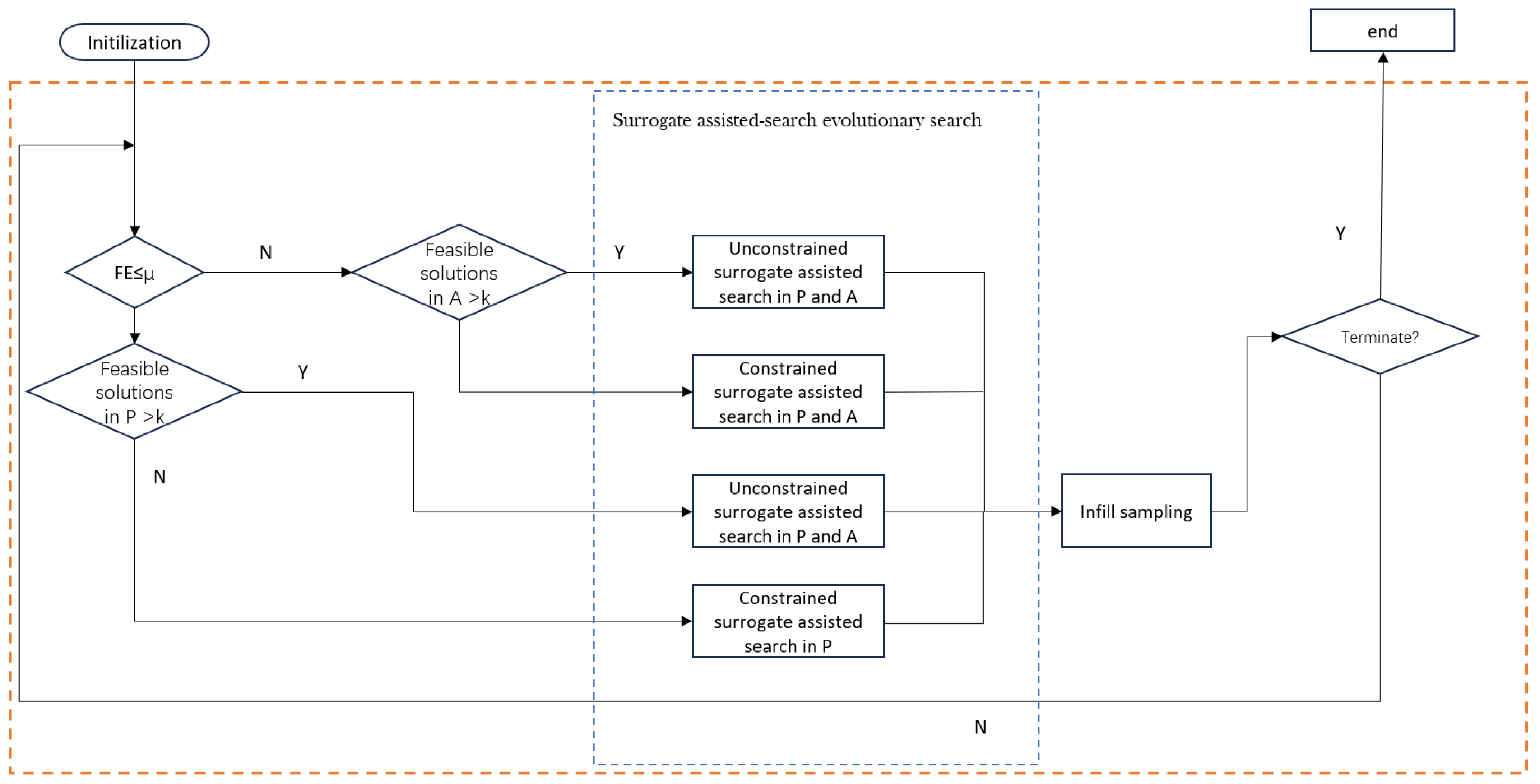
To solve the above problems, we propose a preference model-based surrogate-assisted constrained multi-objective evolutionary algorithm, which performs different offspring generation strategies based on the current difficulty of finding a feasible solution. In addition, a surrogate model management strategy is used to adjust the surrogate model evaluation strategy and the new offspring selection strategy according to the performance of the current surrogate model. Specifically, this paper’s contributions are as follows:

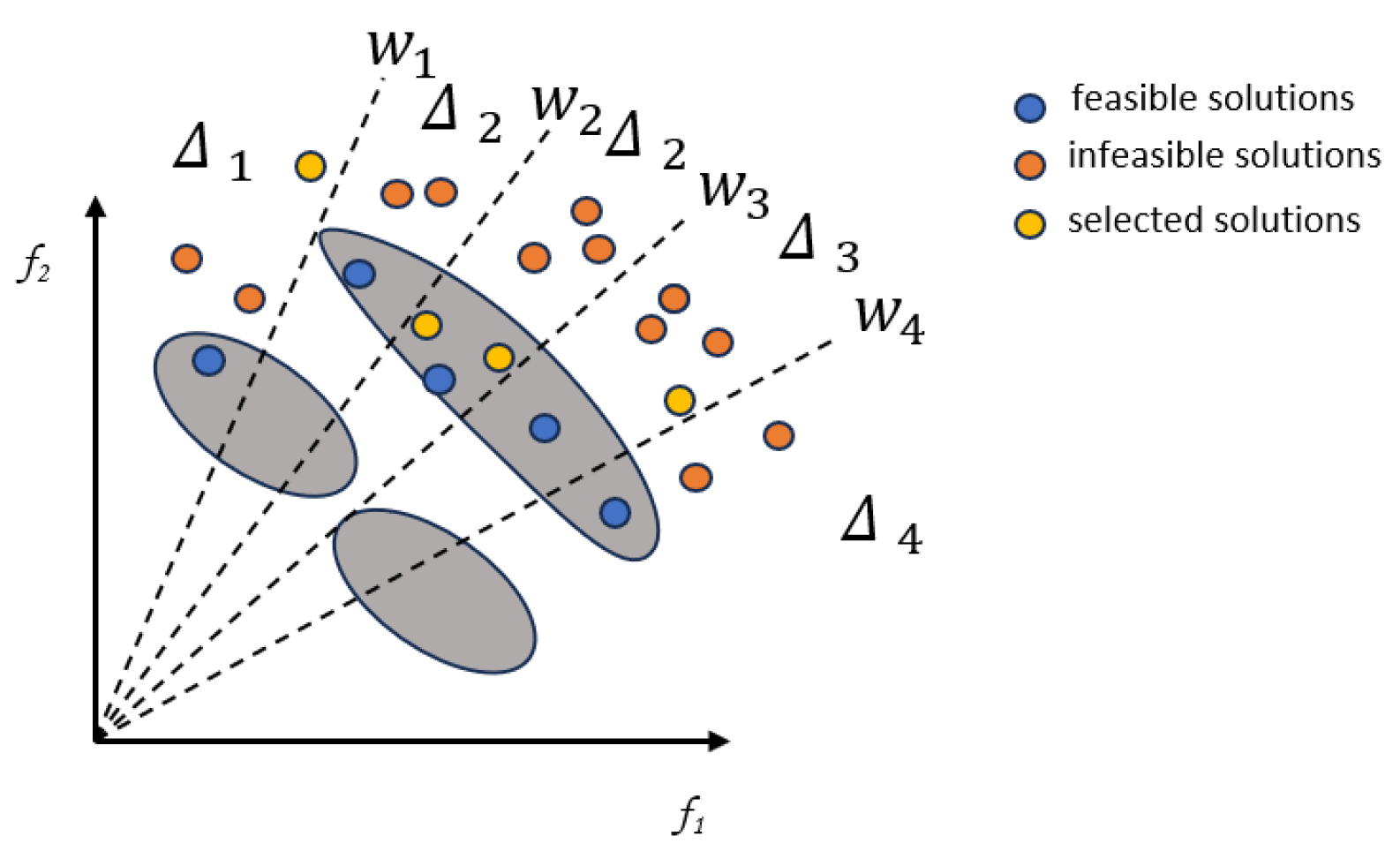
• To meet the optimization requirements of the population at different stages, we propose a multi-preference search model based on evolutionary demands. In the early stage of evolution, the waste of computing resources is reduced by rapidly converging to the feasible region. In the middle stage of evolution, for the feasibility search requirements of the population, a feasible solution archive and constrained preference strategy are used to help the population cross infeasible regions. For the diversity requirements of the population, the objective value preference algorithm is used to help the population get rid of local optima. In the later stage, the model balances diversity and convergence demands to facilitate the exploration and exploitation of feasible regions.
• In surrogate-assisted evolutionary algorithms, the accuracy of the surrogate model plays a crucial role in the algorithm’s performance. To better utilize the surrogate model for evaluating newly generated solutions, a strategy to modify the number of predictions of the surrogate model based on the prediction error of the current realistically evaluated solutions is proposed.
• Target constrained Pareto frontier search and unconstrained Pareto frontier search address the different optimization needs of populations. Convergence to the feasible domain is accelerated by auxiliary populations when the main population lacks feasible solutions and is converted to objective-value dominated to converge across the feasible domain to the unconstrained Pareto front (UPF) when there are sufficient feasible solutions.

2. Preliminaries

2.1. Kriging

In this study, we use the Kriging model to approximate the objective function and constraint functions. As a typical surrogate model, Kriging can effectively fit complex functions and provide uncertainty estimates for the prediction results. The dynamic evaluation strategy relies on the prediction accuracy and uncertainty information of the Kriging model. By monitoring the model prediction errors (such as the mean square error and the feasibility misclassification rate), it dynamically adjusts the usage frequency of the surrogate model. When the model reliability is low, the number of surrogate evaluations is reduced to prevent it from misleading the search direction. When the reliability is high, the number of surrogate evaluations is increased to save computational resources. The mathematical model of the Kriging model can be expressed as:

$$y\left(x\right)=f\left(x\right)+ϵ$$

(3)

where $ϵ\sim \mathcal{N}(\mu ,{\sigma }_n^2)$ is a uniformly distributed Gaussian noise and $\mu$ and $\sigma$ are two constants independent of x.

Given the collected data $X=\{x_1,x_2,\dots ,x_N\}$ and its corresponding output $Y=\{y\left(x_1\right),y\left(x_2\right),\dots ,y\left(x_N\right)\}$, for an unevaluated point $z^{\ast }$, the estimated output $y\left(z^{\ast }\right)$, the mean $\overline{f}\left(z^{\ast }\right)$, and the variance ${\sigma }^2$ are calculated as follows:

$$\overline{f}\left(z^{\ast }\right)=\psi \left(z^{\ast }\right)+k_{\ast }^{\top }{(K+{\sigma }_n^{2}I)}^{-1}(Y-\psi \left(X\right))$$

(4)

$${\sigma }^2\left(z^{\ast }\right)=k(z^{\ast },z^{\ast })-k_{\ast }^{\top }{(K+{\sigma }_n^{2}I)}^{-1}{k}_{\ast }$$

(5)

Among others, X is the average vector of X, the mean vector of $k^{\ast }$ is the average vector of X, and $z^{\ast }$ is the vector of covariances between K, where K is the covariance matrix of X. The covariance matrix of two data points is measured using the squared exponential function as the covariance function of X and $X^{\prime }$. The similarity between the two data points X and $X^{\prime }$ is given by:

$$k(x,x^{\prime })=\theta exp\left(-{\displaystyle \frac{1}{2{\ell }^2}}{(x-x^{\prime })}^{\top }(x-x^{\prime })\right).$$

(6)

Predicting the mean $\overline{f}\left(z^{\ast }\right)$ is directly used as $y\left(z^{\ast }\right)$, the predicted value, and the predicted variance ${\sigma }^2\left[f\left(z^{\ast }\right)\right]$ represents the uncertainty. The hyperparameters in the covariance function can be obtained by maximizing the log-marginal likelihood function as follows:

$$logp(Y\mid X)=-{\displaystyle \frac{1}{2}}{(Y-m\left(X\right))}^{\top }{(K+{\delta }_n^{2}I)}^{-1}(Y-m\left(X\right))-{\displaystyle \frac{1}{2}}log|K+{\delta }_n^{2}I|-{\displaystyle \frac{N}{2}}log2\pi .$$

(7)

2.2. Co-Evolution

In this study, we introduce the co-evolutionary algorithm into the multi-preference search mode based on evolutionary demand. Through the co-evolution of the main population and the auxiliary population, the overall optimization performance is enhanced. This collaborative mechanism enables the algorithm to dynamically balance feasibility and convergence at different stages of evolution. The cooperative co-evolutionary algorithm is an optimization method based on evolutionary algorithms. Its main aim is to decompose a complex problem into several relatively simple sub-problems, solve these sub-problems separately, and then combine their solutions to obtain the overall solution. During this process, the solutions of different sub-problems interact with each other through cooperation and competition, thereby optimizing the overall problem.

The basic steps of the co-evolutionary algorithm are as follows:

Problem decomposition: Decompose the original problem into multiple subproblems. These sub-problems should be relatively independent and can be solved relatively easily.

Individual representation: Designing a suitable individual representation for each subproblem, usually by encoding the solution of the subproblem as an individual.

Subproblem solving: Use evolutionary algorithms (e.g., Genetic Algorithm, Particle Swarm Algorithm, etc.) to solve each subproblem separately, and get the local optimal solution of each subproblem.

Merging and competition: Combining locally optimal solutions to individual subproblems and influencing each other competitively or collaboratively to further optimize those solutions.

Iterative optimization: The above steps are repeated until the stopping condition is reached (e.g., the maximum number of iterations is reached, the convergence condition is satisfied, etc.).

The advantage of the co-evolutionary algorithm is that it can deal with complex, high-dimensional problems and make full use of the structural information of the problem to improve the solution efficiency. It is often used in multi-objective optimization, large-scale optimization, and optimization problems with complex structures.

3. Proposed Methodology

In this section, we propose a surrogate-assisted multi-preference constrained multi-objective evolutionary algorithm (SA-MPCMOEA) designed to address complex constrained multi-objective optimization problems (CMOPs). The primary goal of SA-MPCMOEA is to balance the evolution between feasible and infeasible solutions, facilitating the population to efficiently approach the constrained Pareto front while considering the trade-offs between objective values and constraint violations. Feng et al. [23] proposed the idea of a multi-preference model. This paper designs three different preference models according to the computational resources consumed by the algorithm and the ratio of diversity, convergence, and feasibility, as shown in Figure 1. It uses different offspring generation strategies for each model to guide the evolutionary direction of the population.

3.1. Overview of SA-MPCMOEA

Algorithm 1 summarizes the main procedure of SA-MPCMOEA. In the evolutionary process, SA-MPCMOEA relies on the following three key mechanisms:

• Multi-preference search mode based on evolutionary demand: To coordinate the trade-off between constraint feasibility and objective optimization across different stages of evolution, three preference-based search modes are proposed and switched adaptively based on population feedback. Mode 1 emphasizes the rapid discovery of feasible solutions. Mode 2 simultaneously guides the population toward both the constrained Pareto front and the unconstrained Pareto front. Mode 3 focuses on accelerating convergence when sufficient feasible solutions exist. This mechanism enhances the algorithm’s ability to balance feasibility and optimality across different evolution phases.
• Dynamic assessment strategy: In each generation: Candidate solutions are first evaluated by the surrogate models in terms of both objective and constraint functions. Their prediction confidence is then estimated based on model errors. When the surrogate prediction is reliable, more solutions are evaluated using the surrogate models to save computational resources. Otherwise, the proportion of real evaluations is increased to prevent misleading search directions.This strategy achieves a dynamic balance between solution accuracy and computational efficiency, improving overall optimization performance.
• Fill sampling strategy based on optimization requirements: During the population update phase: A hybrid sampling scheme is adopted, combining uncertainty maximization with potential promising solutions. The former enhances global model performance. The latter steers the population toward potentially optimal regions. Candidate solutions that are too close to the current population are excluded. This improves the diversity and spatial distribution of the population and avoids premature convergence.

These three components work in synergy throughout different stages of surrogate-assisted evolution, enabling SA-MPCMOEA to demonstrate enhanced adaptability and convergence performance on constrained multimodal multi-objective optimization problems.

Algorithm 1 Pseudo-code for the proposed algorithm

Require: Population P; archive A Ensure: P; A; New samples O   1: $C_{\mathrm{pop}}\leftrightarrow P$   2: $w=1$; $w_{\max }=10$   3: Train global model for objective functions and constraint functions.   4: $\mathrm{Search-mode}=\mathrm{condition}(P,A)$   5: while $w\le w_{\max }$ do   6:    if $\mathrm{Search-mode}=0$ then   7:       $\mathrm{Parents}\leftarrow \mathrm{Matingselection}0(P,A)$   8:    else if $\mathrm{Search-mode}=1$ then   9:       $\mathrm{Parents}\leftarrow \mathrm{Matingselection}1\left(P\right)$ 10:    else 11:       $\mathrm{Parents}\leftarrow \mathrm{Matingselection}2(P,A)$ 12:    end if 13:    $\mathrm{Off}\leftarrow \mathrm{Reproduction}\left(\mathrm{Parents}\right)$ 14:    Evaluate Off using surrogate models. 15:    $w_{\max }=\mathrm{Changewmax}$ 16:    Update $C_{\mathrm{pop}}$ with Off. 17: end while 18: $X\leftarrow \mathrm{Sampling}(P,A)$ 19: Add X to P.

3.2. Multi-Preference Search Mode Based on Evolutionary Demand

Constrained multi-objective optimization problems (CMOPs) often contain conflicting objectives and constraint satisfaction requirements. The algorithms’ different preferences for handling objective optimization and constraint optimization at different stages of population evolution directly affect the viability, diversity, and convergence of the population. It is challenging for CMOPs to maintain a balance between using objective information to accelerate convergence and locating feasible regions. Thus, to address the above challenges, we use a multi-preference model to rationalize the scheduling of offspring generation for populations. Based on the idea of the multi-preference model proposed by [24], this paper designs three different preference models according to the computational resources consumed by the algorithm and the ratio of diversity, convergence, and feasibility, as shown in Figure 1. Different offspring generation strategies are used for each model to guide the evolutionary direction of the population.

$$\begin{array}{c}\hfill search\_mode=\left\{\begin{array}{cc}1,\hfill & \mathrm{if}\mathrm{FE}<\alpha ·\mathrm{maxFE}\wedge \mathrm{feasible}\left(P\right)<k,\hfill \\ 3,\hfill & \mathrm{if}\mathrm{FE}<\alpha ·\mathrm{maxFE}\wedge \mathrm{feasible}\left(P\right)\ge k,\hfill \\ 2,\hfill & \mathrm{if}\mathrm{FE}\ge (1-\alpha )·\mathrm{maxFE}\wedge \mathrm{feasible}\left(A\right)<k,\hfill \\ 3,\hfill & \mathrm{if}\mathrm{FE}\ge (1-\alpha )·\mathrm{maxFE}\wedge \mathrm{feasible}\left(A\right)\ge k.\hfill \end{array}\right.\end{array}$$

(8)

where FE represents the number of function evaluations currently used, maxFE represents the maximum number of function evaluations, $\alpha$ is the threshold adjustment parameter, and feasible(·) represents the number of feasible solutions in the population.

3.2.1. Search Mode 1: Angle-Based Convergence Model for Feasible Domains

In Mode 1, the main population P is responsible for exploring the feasible domain, and the auxiliary population A is used to store the feasible solutions of P. A sampling strategy based on the direction of convergence is designed to enhance the convergence of P and feasible selection pressure. In the decision space, based on the solution $x_1$, two convergence directions are formed by the lower bounds L and $x_1$ and the upper bound U and $x_1$.

$$\begin{array}{cc}\hfill v^{(l,x_1)}& =x_1-L\hfill \end{array}$$

(9)

$$\begin{array}{cc}\hfill v^{(u,x_1)}& =x_1-U\hfill \end{array}$$

(10)

Afterwards, the solution is generated by sampling at different step sizes in the direction of convergence:

$$\begin{array}{cc}\hfill X_j^{(l,X_1)}& =L+s_j^l·{\displaystyle \frac{v^{(l,X_1)}}{\parallel v^{(l,X_1)}\parallel }}\hfill \end{array}$$

(11)

$$\begin{array}{cc}\hfill X_k^{(u,X_1)}& =U+s_k^u·{\displaystyle \frac{v^{(u,X_1)}}{\parallel v^{(u,X_1)}\parallel }}\hfill \end{array}$$

(12)

where $s_j^l$ and $s_k^u\in [0,\parallel U-L\parallel ]$ denote the step size, j and k denote the first j times and the k times sampling, and $\parallel ·\parallel$ denotes the Euclidean distance.

3.2.2. Search Mode 2: Co-Evolutionary Search Model

In Mode 2, the main population and the auxiliary population are respectively used to explore the satisfaction demands of constraint conditions and the optimization demands of objective values. After the main population P and the auxiliary population A independently generate offspring solutions, the main population selects the solution with a lower CV value to approach the constrained Pareto front, and the auxiliary population selects the solution with a better objective value to approach the unconstrained Pareto front. In the population update operation, the main population P is first combined with the auxiliary population A. For updating P, feasible solutions are prioritized; if insufficient feasible solutions exist, the solution with the smallest CV value is selected. For updating A, non-dominated sorting and crowded distance are used to select individuals with better diversity and convergence to help the population cross the feasible region and improve diversity.

3.2.3. Search Mode 3: Feasible Domain-Assisted Exploration Search Model

Population P in Mode 3 continues to evolve, driven by feasibility criteria, and population A is designed to help the population explore unexplored areas of population P. The two mating parents are from population P and population A. The offspring are produced from population P and population A and are used to renew population P and population A.

Population A does not consider constraint values and is driven by diversity and convergence information. Population A is mixed with child Q to generate a mixed population H. The solutions in population H and population P are then compared with a reference vector based on the reference vector $w_i$ of the subregion ${\Delta }_i$ associated with them. For each subregion, if no solution exists in population P, the optimal non-dominated solution in H is selected in population A. The optimal non-dominated solution in H is then selected in population A.

Figure 2 illustrates the individual selection mechanism of Model 3. In the diagram, blue dots represent individuals selected by Population P, while yellow dots denote those selected by Population A.

3.3. Dynamic Assessment Strategy

In expensive problems, due to limited computational resources, it is necessary to conserve computational resources by evaluating candidate solutions using surrogate models. The reliability of the surrogate model varies for different stages of the algorithm. When the reliability of the surrogate model is low, the objective values and constraint violations obtained by evaluating the candidate solutions using the surrogate model may have large errors with the real values, and it is difficult to truly reflect the superiority of a candidate solution among all the offspring solutions, which leads to the algorithm selecting a solution that cannot help the population to advance to the CPF, which results in a waste of real evaluation resources. Therefore, when the reliability of the surrogate model is low, the number of surrogate evaluations of the surrogate model should be reduced to avoid misleading the direction of population evolution. To this end, this paper dynamically adjusts the number of model evaluations according to the mean square error (MSE) of the surrogate model prediction results and the results of the real evaluation with the evaluation errors. The error bounds in Kriging models are determined by the MSE and the correlation index. The MSE is used to evaluate the prediction accuracy of the model, with a lower MSE indicating a better fit [25]. When the prediction error rate is high, the reliability of the surrogate model is considered to be low. At this point, the number of surrogate model evaluations is reduced, and when the surrogate model evaluation error rate is low, the number of surrogate model evaluations is increased. In [26], Song et al. proved that the change of $w_{\max }$ will greatly affect the performance of the surrogate-assisted evolutionary algorithm.

$$w_{\max }=\lambda \left({\displaystyle \frac{1}{{\sum }_{i=1}^S{\mathrm{MSE}}_i}}\right)$$

(13)

where $w_{\max }$ is the maximum number of evaluations of the surrogate model, S is the number of candidate solutions, and $\lambda$ is the scaling factor.

3.4. Fill Sampling Strategy Based on Optimization Requirements

The newly generated solutions serve two purposes for the surrogate model-assisted evolutionary algorithm: (1) They can select candidate solutions with maximum uncertainty as training data to improve the accuracy of the surrogate model. (2) They can select candidate solutions that outperform the current evaluation under feasible rules, i.e., potentially good solutions, to find optimal solutions [16,17,27].

One of the advantages of the Kriging model is that it can provide not only a prediction of the unknown function but also an estimate of the error in the prediction. The solution with the largest error in the predicted value is the maximum uncertainty solution, indicating that the surrogate model has low confidence in its predictions around that solution. Sampling such solutions can improve the global accuracy of the surrogate model. Potentially good solutions are located around the approximate landscape [28]. Sampling such solutions can help the population find the optimal solution.

Based on the above considerations, the solution for true function evaluation in surrogate-assisted evolutionary algorithms should take both factors into account. To accelerate the speed of the population to find a feasible solution and avoid the population from falling into a local optimum, the solutions whose distance from the current population in the decision space is less than a set value are eliminated to optimize the distribution of the population in the decision space. The search for the optimal solution in this paper is measured by calculating the convergence information and diversity information of the solution. Among them, $S_1$ is used to solve the CPF search problem.

$$S_1\left(x\right)=\mathrm{argmax}\left(R_x+{\displaystyle \frac{1}{\mathrm{dist}(x,x^{\prime })+2}}\right)$$

(14)

where $R_x$ denotes the number of individuals that x dominates, $\mathrm{dist}(x,x^{\prime })$ denotes the Euclidean distance between the solutions x and $x^{\prime }$, and ${\displaystyle \frac{1}{\mathrm{dist}(x,x^{\prime })+2}}$ represents the diversity information of the solution x. After that, we divide the candidate solutions into k clusters using the k-nearest neighbor algorithm and select a solution with minimum fitness from each cluster for expensive evaluation.

For the UPF (Unconstrained Pareto Front) exploration, we give the objective function a higher priority and therefore do not consider the constraint values. Thus, in the $S_1$ diversity information, we multiply the distance by the difference of the constraint values.

$$S_2\left(x\right)=\mathrm{argmax}\left(R_x+{\displaystyle \frac{CV\left(x\right)-CV\left(x^{\prime }\right)}{\mathrm{dist}(x,x^{\prime })+2}}\right)$$

(15)

4. Experimental Setup

In this paper, to demonstrate the ability of SA-MPCMOEA to solve expensive constrained multi-objective problems, two test suites, CF and LIRCMOP, are used to compare SA-MPCMOEA with the current state-of-the-art algorithms. The number of decision variables is set to 10 for all test instances. It is assumed that the evaluation of their objectives and constraints is expensive. The performance of the algorithms is evaluated using IGD metrics

$$\mathrm{IGD}(S_f,S^{\ast })={\displaystyle \frac{1}{|S^{\ast }|}}\sum _{x\in S^{\ast }}\mathrm{dis}(x,S_f)$$

(16)

where $\mathrm{dis}(x,S_f)$ denotes the minimum Euclidean distance from x to $S_f$ and $|S^{\ast }|$ denotes the number of points in $S^{\ast }$. A total of 10,000 reference points are used to compute the IGD values. Smaller IGD values indicate better convergence and diversity of the algorithm’s non-dominated set.

The hypervolume (HV) is a metric used to measure the volume of the objective space covered by a solution set relative to a reference point. A larger HV value indicates that the solution set obtained by the algorithm covers a wider range of the true Pareto front, demonstrating better solution quality and algorithm efficiency. The HV calculation method is shown in the following equation:

$$HV\left(A\right)=\lambda \left(\bigcup _{i=1}^{\left|S\right|}{v}_i\right)$$

(17)

where $\lambda$ denotes the Lebesgue measure, S represents the non-dominated solution set, and $v_i$ represents the hypervolume formed by the reference point and the non-dominated solutions. In this paper, we adopt the nadir point method for reference point selection, which uses the maximum value of all objective functions as the reference point. The advantage of the HV indicator lies in its ability to be calculated without prior knowledge of the true Pareto front of test problems, making it particularly suitable for real-world applications.

To ensure the fairness of the experiments, the parameter settings for all compared algorithms are configured as follows:

• All algorithms are independently executed 30 times.
• The maximum number of real function evaluations for each algorithm is set to 1000.
• The population size is uniformly set to 100 across all test problems.

4.1. Experiments Results

In this section, our algorithm SA-MPCMOEA is compared with the following state-of-the-art algorithms: The proposed SA-MPCMOEA was empirically compared with six state-of-the-art CMOEAs: CTAEA [29], RVEAa [30], ABSAEA, CCMO, and NSGA-II. to examine its performance.

All compared algorithms were implemented in MATLAB (R2023a) within the PlatEMO platform [31] and executed on a computer equipped with a 13th Gen Intel Core i5-13400 2.50 GHz CPU and the Microsoft Windows 10 operating system.

• CTAEA balances convergence, diversity, and feasibility by maintaining two collaborative archives: the convergence-oriented archive (CA) and the diversity-oriented archive (DA). By adaptively selecting individuals from these archives based on their distinct evolutionary states to generate offspring solutions, the algorithm achieves superior performance on constrained multi-objective optimization problems.
• RVEAa employs a reference vector regeneration strategy to address constrained many-objective optimization problems with irregular PFs (Pareto Fronts) and utilizes the angle-penalized distance to maintain a balance between convergence and diversity.
• ABSAEA employs an adaptive Bayesian surrogate-assisted evolutionary algorithm to address expensive multi-objective optimization problems, where the hyperparameters of the acquisition function are dynamically tuned to select candidate solutions for real function evaluations, thereby reducing the computational cost of evaluations.
• CMOEAD ensures the diversity of solutions by performing niching operations on individuals within the population. Through the adaptive updating of reference points, the CMOEAD algorithm can simultaneously search for multiple Pareto-optimal points in a single run to achieve efficient exploration.
• NSGA-II improves computational efficiency by utilizing fast non-dominated sorting and an enhanced dominance mechanism. Owing to its selection operator, which constructs the mating pool based on fitness and distribution characteristics, the algorithm achieves well-distributed solution sets across most optimization problems while demonstrating superior convergence performance near the true Pareto-optimal front in practical scenarios.

4.1.1. The Computational Complexity of SA-MPCMOEA

When using the Kriging model, the time complexity of the algorithm is mainly determined by the surrogate model training. The model training of Kriging requires the calculation of the inverse of the covariance matrix, and the time complexity is $O\left(N^3\right)$, where N is the population size. The independent modeling of each objective function increases the total training cost to $O\left(M{N}^3\right)$ (M is the dimension of the objective function). In each iteration, the surrogate prediction of the offspring individuals requires $O\left(MN\right)$ time (traversing M models, and the single prediction complexity of each model is $O\left(N\right)$). The overall complexity is $O(M{N}^3+TMN)$, where T is the number of iterations. As shown in

Table 1. Runtime comparison.

Problem	M	D	NSGAII	RVEAa	CTAEA	CCMO	ABSAEA	SA-MPCMOEA
CF1	2	10	6.89 × ${10}^{-2}$ (s)	5.04 × ${10}^{-1}$ (s)	1.66 × ${10}^{+0}$ (s)	2.05 × ${10}^{-1}$ (s)	8.89 × ${10}^{+0}$ (s)	1.07 × ${10}^{+1}$ (s)
CF2	2	10	2.35 × ${10}^{-2}$ (s)	3.51 × ${10}^{-2}$ (s)	1.49 × ${10}^{+0}$ (s)	1.57 × ${10}^{-1}$ (s)	1.48 × ${10}^{+2}$ (s)	1.52 × ${10}^{+2}$ (s)
CF3	2	10	1.84 × ${10}^{-2}$ (s)	3.35 × ${10}^{-2}$ (s)	1.32 × ${10}^{+0}$ (s)	1.39 × ${10}^{-1}$ (s)	1.22 × ${10}^{+2}$ (s)	1.35 × ${10}^{+2}$ (s)
CF4	2	10	1.99 × ${10}^{-2}$ (s)	3.72 × ${10}^{-2}$ (s)	1.55 × ${10}^{+0}$ (s)	1.44 × ${10}^{-1}$ (s)	4.06 × ${10}^{+1}$ (s)	1.98 × ${10}^{+2}$ (s)
CF5	2	10	2.05 × ${10}^{-2}$ (s)	3.72 × ${10}^{-2}$ (s)	1.57 × ${10}^{+0}$ (s)	1.49 × ${10}^{-1}$ (s)	1.26 × ${10}^{+2}$ (s)	1.78 × ${10}^{+2}$ (s)
CF6	2	10	2.34 × ${10}^{-2}$ (s)	3.93 × ${10}^{-2}$ (s)	1.54 × ${10}^{+0}$ (s)	1.63 × ${10}^{-1}$ (s)	1.33 × ${10}^{+2}$ (s)	1.30 × ${10}^{+2}$ (s)
CF7	2	10	2.11 × ${10}^{-2}$ (s)	3.64 × ${10}^{-2}$ (s)	1.47 × ${10}^{+0}$ (s)	1.33 × ${10}^{-1}$ (s)	3.21 × ${10}^{+1}$ (s)	4.06 × ${10}^{+1}$ (s)
CF8	3	10	4.64 × ${10}^{-2}$ (s)	4.74 × ${10}^{-2}$ (s)	1.19 × ${10}^{+0}$ (s)	1.23 × ${10}^{-1}$ (s)	4.17 × ${10}^{+1}$ (s)	6.55 × ${10}^{+1}$ (s)
CF9	3	10	1.96 × ${10}^{-2}$ (s)	4.12 × ${10}^{-2}$ (s)	1.30 × ${10}^{+0}$ (s)	1.26 × ${10}^{-1}$ (s)	4.27 × ${10}^{+1}$ (s)	8.77 × ${10}^{+1}$ (s)
CF10	3	10	3.25 × ${10}^{-2}$ (s)	3.58 × ${10}^{-2}$ (s)	1.07 × ${10}^{+0}$ (s)	1.13 × ${10}^{-1}$ (s)	4.78 × ${10}^{+1}$ (s)	6.97 × ${10}^{+1}$ (s)
LIRCMOP1	2	30	2.11 × ${10}^{-1}$ (s)	1.78 × ${10}^{-1}$ (s)	1.43 × ${10}^{+0}$ (s)	1.92 × ${10}^{-1}$ (s)	4.97 × ${10}^{+3}$ (s)	9.03 × ${10}^{+3}$ (s)
LIRCMOP2	2	30	9.55 × ${10}^{-2}$ (s)	5.96 × ${10}^{-2}$ (s)	1.26 × ${10}^{+0}$ (s)	1.16 × ${10}^{-1}$ (s)	2.90 × ${10}^{+3}$ (s)	8.85 × ${10}^{+3}$ (s)
LIRCMOP3	2	30	8.72 × ${10}^{-2}$ (s)	5.07 × ${10}^{-2}$ (s)	1.06 × ${10}^{+0}$ (s)	1.12 × ${10}^{-1}$ (s)	8.42 × ${10}^{+2}$ (s)	9.17 × ${10}^{+3}$ (s)
LIRCMOP4	2	30	8.50 × ${10}^{-2}$ (s)	4.59 × ${10}^{-2}$ (s)	1.08 × ${10}^{+0}$ (s)	1.12 × ${10}^{-1}$ (s)	8.72 × ${10}^{+2}$ (s)	6.85 × ${10}^{+2}$ (s)
LIRCMOP5	2	30	6.00 × ${10}^{-2}$ (s)	5.49 × ${10}^{-2}$ (s)	1.38 × ${10}^{+0}$ (s)	1.49 × ${10}^{-1}$ (s)	1.57 × ${10}^{+3}$ (s)	3.88 × ${10}^{+2}$ (s)
LIRCMOP6	2	30	5.42 × ${10}^{-2}$ (s)	5.29 × ${10}^{-2}$ (s)	1.39 × ${10}^{+0}$ (s)	1.47 × ${10}^{-1}$ (s)	1.16 × ${10}^{+3}$ (s)	5.63 × ${10}^{+3}$ (s)
LIRCMOP7	2	30	5.66 × ${10}^{-2}$ (s)	4.76 × ${10}^{-2}$ (s)	1.29 × ${10}^{+0}$ (s)	1.46 × ${10}^{-1}$ (s)	1.71 × ${10}^{+3}$ (s)	3.10 × ${10}^{+2}$ (s)
LIRCMOP8	2	30	5.66 × ${10}^{-2}$ (s)	4.72 × ${10}^{-2}$ (s)	1.30 × ${10}^{+0}$ (s)	1.47 × ${10}^{-1}$ (s)	5.71 × ${10}^{+2}$ (s)	6.30 × ${10}^{+3}$ (s)
LIRCMOP9	2	30	5.10 × ${10}^{-2}$ (s)	4.75 × ${10}^{-2}$ (s)	1.36 × ${10}^{+0}$ (s)	1.46 × ${10}^{-1}$ (s)	4.60 × ${10}^{+2}$ (s)	7.08 × ${10}^{+2}$ (s)
LIRCMOP10	2	30	5.12 × ${10}^{-2}$ (s)	5.50 × ${10}^{-2}$ (s)	1.38 × ${10}^{+0}$ (s)	1.45 × ${10}^{-1}$ (s)	5.36 × ${10}^{+2}$ (s)	1.04 × ${10}^{+3}$ (s)
LIRCMOP11	2	30	5.18 × ${10}^{-2}$ (s)	5.01 × ${10}^{-2}$ (s)	1.45 × ${10}^{+0}$ (s)	1.45 × ${10}^{-1}$ (s)	7.55 × ${10}^{+2}$ (s)	2.58 × ${10}^{+3}$ (s)
LIRCMOP12	2	30	5.38 × ${10}^{-2}$ (s)	4.80 × ${10}^{-2}$ (s)	1.37 × ${10}^{+0}$ (s)	1.56 × ${10}^{-1}$ (s)	1.31 × ${10}^{+3}$ (s)	5.33 × ${10}^{+1}$ (s)
LIRCMOP13	3	30	5.59 × ${10}^{-2}$ (s)	6.31 × ${10}^{-2}$ (s)	1.67 × ${10}^{+0}$ (s)	1.47 × ${10}^{-1}$ (s)	2.72 × ${10}^{+4}$ (s)	1.14 × ${10}^{+4}$ (s)
LIRCMOP14	3	30	5.05 × ${10}^{-2}$ (s)	5.43 × ${10}^{-2}$ (s)	1.46 × ${10}^{+0}$ (s)	1.49 × ${10}^{-1}$ (s)	1.03 × ${10}^{+3}$ (s)	1.35 × ${10}^{+4}$ (s)

, SA-MPCMOEA is compared with other algorithms on CF test problems and LIRCMOP test problems, respectively. Using 1000 evaluations, each algorithm is independently run once.

4.1.2. Result on CF Test Suit

The comparative results of SA-MPCMOEA and other algorithms on the CF test problems [32] are presented in

Table 2. Performance comparison of different algorithms on CF problems.

Problem	M	D	NSGAII	RVEAa	CTAEA	CCMO	ABSAEA	SA-MPCMOEA
CF1	2	10	2.6034 × ${10}^{-1}$ (3.31 × ${10}^{-2}$) −	3.7454 × ${10}^{-1}$ (2.15 × ${10}^{-1}$) −	2.6208 × ${10}^{-1}$ (2.84 × ${10}^{-2}$) −	1.5170 × ${10}^{-1}$ (1.70 × ${10}^{-2}$) =	1.2604 × ${10}^{-1}$ (1.39 × ${10}^{-2}$) +	1.4323 × ${10}^{-1}$ (3.39 × ${10}^{-2}$)
CF2	2	10	5.8261 × ${10}^{-1}$ (1.21 × ${10}^{-1}$) −	1.9134 × ${10}^{-1}$ (8.21 × ${10}^{-2}$) −	5.9542 × ${10}^{-1}$ (1.45 × ${10}^{-1}$) −	2.7130 × ${10}^{-1}$ (6.11 × ${10}^{-2}$) −	1.7853 × ${10}^{-1}$ (8.15 × ${10}^{-2}$) −	9.3409 × ${10}^{-2}$ (3.66 × ${10}^{-2}$)
CF3	2	10	5.0399 × ${10}^{+0}$ (1.04 × ${10}^{+0}$) −	1.4482 × ${10}^{+0}$ (4.08 × ${10}^{-1}$) =	5.1533 × ${10}^{+0}$ (1.19 × ${10}^{+0}$) −	2.3337 × ${10}^{+0}$ (5.44 × ${10}^{-1}$) −	8.8452 × ${10}^{-1}$ (2.85 × ${10}^{-1}$) +	1.3541 × ${10}^{+0}$ (1.92 × ${10}^{-1}$)
CF4	2	10	2.2062 × ${10}^{+0}$ (5.80 × ${10}^{-1}$) −	4.9490 × ${10}^{-1}$ (4.29 × ${10}^{-1}$) −	2.3354 × ${10}^{+0}$ (5.26 × ${10}^{-1}$) −	8.1789 × ${10}^{-1}$ (2.25 × ${10}^{-1}$) −	4.0095 × ${10}^{-1}$ (1.56 × ${10}^{-1}$) −	2.1887 × ${10}^{-1}$ (1.13 × ${10}^{-1}$)
CF5	2	10	8.5810 × ${10}^{+0}$ (1.19 × ${10}^{+0}$) −	2.5154 × ${10}^{+0}$ (3.58 × ${10}^{+0}$) −	8.6420 × ${10}^{+0}$ (1.45 × ${10}^{+0}$) −	3.8500 × ${10}^{+0}$ (7.35 × ${10}^{-1}$) −	1.5993 × ${10}^{+0}$ (1.06 × ${10}^{+0}$) =	1.4593 × ${10}^{+0}$ (6.88 × ${10}^{-1}$)
CF6	2	10	2.7177 × ${10}^{+0}$ (6.39 × ${10}^{-1}$) −	3.0682 × ${10}^{-1}$ (9.76 × ${10}^{-2}$) −	2.4063 × ${10}^{+0}$ (6.63 × ${10}^{-1}$) −	6.0600 × ${10}^{-1}$ (1.99 × ${10}^{-1}$) −	2.1663 × ${10}^{-1}$ (9.33 × ${10}^{-2}$) −	1.0405 × ${10}^{-1}$ (5.11 × ${10}^{-2}$)
CF7	2	10	9.2139 × ${10}^{+0}$ (1.61 × ${10}^{+0}$) −	2.6008 × ${10}^{+0}$ (1.77 × ${10}^{+0}$) −	9.5777 × ${10}^{+0}$ (1.53 × ${10}^{+0}$) −	4.7972 × ${10}^{+0}$ (9.56 × ${10}^{-1}$) −	2.6581 × ${10}^{+0}$ (2.23 × ${10}^{+0}$) −	1.6372 × ${10}^{+0}$ (8.31 × ${10}^{-1}$)
CF8	3	10	1.3560 × ${10}^{+1}$ (7.63 × ${10}^{+0}$) −	9.8810 × ${10}^{-1}$ (8.48 × ${10}^{-1}$) −	1.2076 × ${10}^{+1}$ (7.59 × ${10}^{+0}$) −	3.2466 × ${10}^{+0}$ (4.24 × ${10}^{+0}$) −	5.1684 × ${10}^{-1}$ (1.64 × ${10}^{-1}$) =	5.3287 × ${10}^{-1}$ (1.54 × ${10}^{-1}$)
CF9	3	10	1.8522 × ${10}^{+0}$ (5.46 × ${10}^{-1}$) −	3.8735 × ${10}^{-1}$ (1.01 × ${10}^{-1}$) −	1.7399 × ${10}^{+0}$ (5.81 × ${10}^{-1}$) −	6.4976 × ${10}^{-1}$ (1.32 × ${10}^{-1}$) −	2.6450 × ${10}^{-1}$ (5.69 × ${10}^{-2}$) =	2.4954 × ${10}^{-1}$ (7.98 × ${10}^{-2}$)
CF10	3	10	1.9259 × ${10}^{+1}$ (0.00 × ${10}^{+0}$) =	3.8359 × ${10}^{+0}$ (2.43 × ${10}^{+0}$) =	NaN (NaN)	2.2408 × ${10}^{+1}$ (9.05 × ${10}^{+0}$) −	2.1613 × ${10}^{+0}$ (1.33 × ${10}^{+0}$) +	5.6216 × ${10}^{+0}$ (2.63 × ${10}^{+0}$)
+/−/=			0/9/1	0/8/2	0/9/0	0/9/1	3/4/3

.

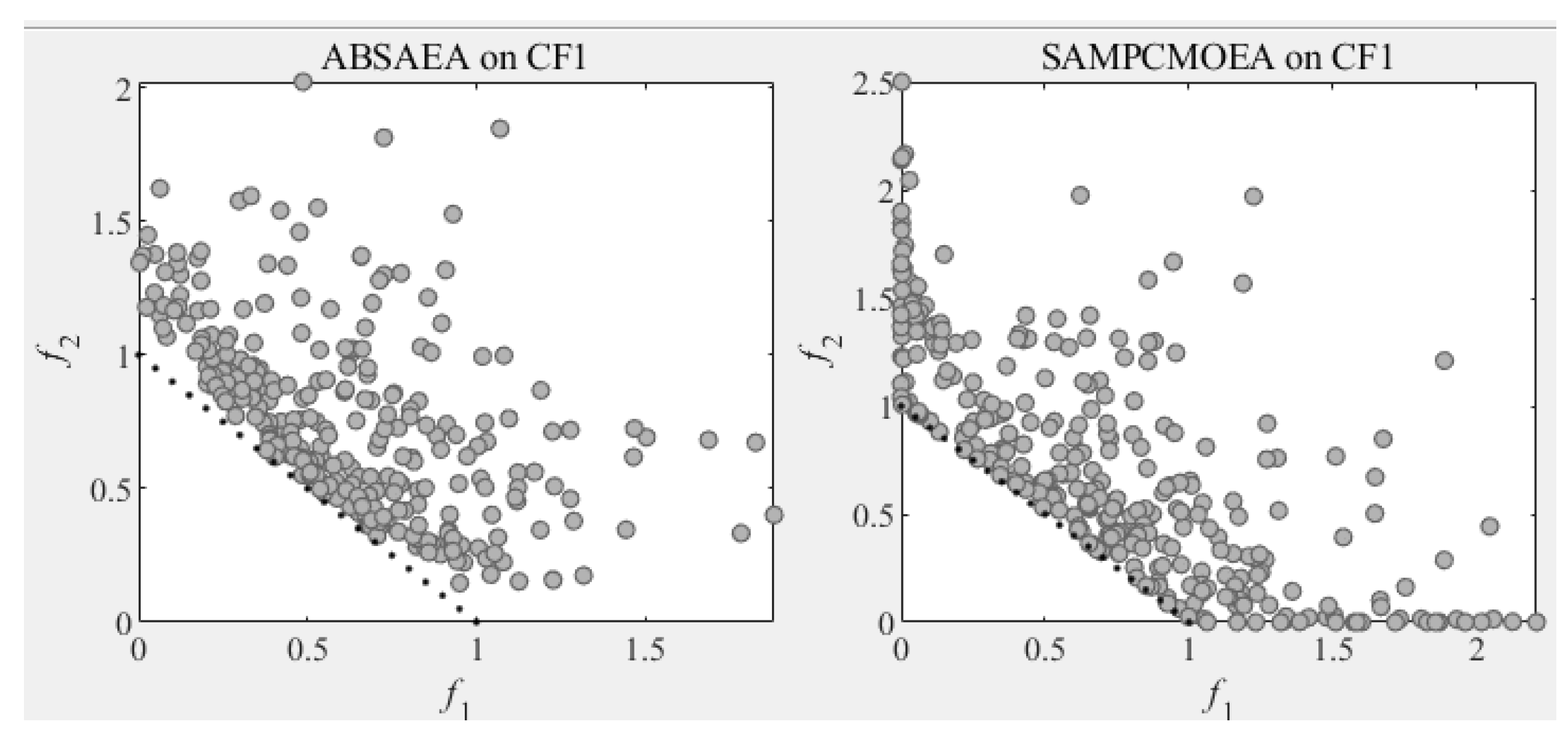
As shown in Table 2, the SA-MPCMOEA algorithm demonstrates a significant advantage across the CF benchmark problems. Among all compared algorithms, SA-MPCMOEA is only outperformed by ABSAEA on three problems (CF1, CF3, and CF10) in terms of IGD values because the feasible region of the problem is relatively large in CF1, CF3, and CF10. SA-MPCMOEA starts to focus on the diversity of the population after finding a sufficient number of feasible solutions, as shown in Figure 3, while maintaining superiority or equivalent performance on the remaining seven problems. Notably, SA-MPCMOEA exhibits exceptional performance on complex constrained problems (CF2, CF4, CF6, and CF7), particularly in the equality-constrained problem CF7, where it achieves the best results, highlighting its robust constraint-handling capability. In high-dimensional problems (CF8, CF9, and CF10), the infeasible regions disrupt the feasible domains, leading to the inferior performance of other algorithms compared to SA-MPCMOEA and ABSAEA. Benefiting from the angle-based convergence model for feasible domains, SA-MPCMOEA efficiently traverses complex and vast search spaces, rapidly crossing infeasible regions to locate feasible solutions.

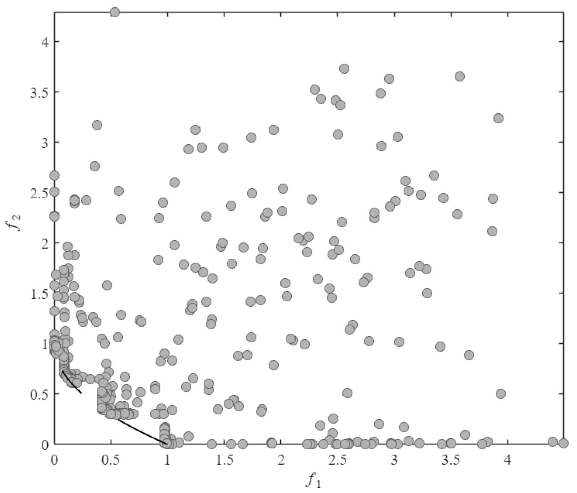
As observed in Figure 4 and Figure 5, SA-MPCMOEA effectively prevents population convergence toward CPF gap regions through its constraint-dominated exploration mechanism when handling problems with a discontinuous constrained Pareto front. Compared to ABSAEA, SA-MPCMOEA achieves more uniform distribution along the CPF, demonstrating superior diversity preservation capabilities in maintaining solution spread.

4.1.3. Result on LIRCMOP Test Suit

The comparative results of SA-MPCMOEA and other algorithms on the LIRCMOP [33] high-dimensional complex constrained multi-objective optimization problems are summarized in

Table 3. Performance comparison of different algorithms on LIRCMOP problems.

Problem	M	D	NSGAII	RVEAa	CTAEA	CCMO	ABSAEA	SA-MPCMOEA
LIRCMOP1	2	30	NaN (NaN)	NaN (NaN)	NaN (NaN)	NaN (NaN)	NaN (NaN)	3.6013 × ${10}^{-1}$ (0.00 × ${10}^{+0}$)
LIRCMOP2	2	30	NaN (NaN)	NaN (NaN)	NaN (NaN)	3.1961 × ${10}^{-1}$ (6.96 × ${10}^{-4}$) =	NaN (NaN)	3.1757 × ${10}^{-1}$ (1.06 × ${10}^{-2}$)
LIRCMOP3	2	30	NaN (NaN)	NaN (NaN)	NaN (NaN)	3.5369 × ${10}^{-1}$ (1.18 × ${10}^{-3}$) =	NaN (NaN)	3.6029 × ${10}^{-1}$ (1.53 × ${10}^{-2}$)
LIRCMOP4	2	30	NaN (NaN)	NaN (NaN)	NaN (NaN)	3.2779× ${10}^{-1}$ (0.00× ${10}^{+0}$) =	NaN (NaN)	3.3316 × ${10}^{-1}$ (1.63 × ${10}^{-2}$)
LIRCMOP5	2	30	1.7325 × ${10}^{+1}$ (2.36 × ${10}^{+0}$) −	4.1995 × ${10}^{+0}$ (1.28 × ${10}^{+0}$) +	8.9478 × ${10}^{+0}$ (1.39 × ${10}^{+0}$) −	7.2675 × ${10}^{+0}$ (1.50 × ${10}^{+0}$) +	1.9014 × ${10}^{+1}$ (2.15 × ${10}^{+0}$) −	7.3039 × ${10}^{+0}$ (9.32 × ${10}^{+0}$)
LIRCMOP6	2	30	1.6264 × ${10}^{+1}$ (2.39 × ${10}^{+0}$) −	4.0626 × ${10}^{+0}$ (9.52 × ${10}^{-1}$) +	8.7980 × ${10}^{+0}$ (1.51 × ${10}^{+0}$) −	7.2434 × ${10}^{+0}$ (1.24 × ${10}^{+0}$) +	1.8519 × ${10}^{+1}$ (2.49 × ${10}^{+0}$) −	7.3403 × ${10}^{+0}$ (9.78 × ${10}^{+0}$)
LIRCMOP7	2	30	1.5999 × ${10}^{+1}$ (2.52 × ${10}^{+0}$) −	4.6797 × ${10}^{+0}$ (1.32 × ${10}^{+0}$) +	7.8052 × ${10}^{+0}$ (1.14 × ${10}^{+0}$) −	7.2302 × ${10}^{+0}$ (1.22 × ${10}^{+0}$) −	1.8492 × ${10}^{+1}$ (1.65 × ${10}^{+0}$) −	4.7424 × ${10}^{+0}$ (8.06 × ${10}^{+0}$)
LIRCMOP8	2	30	1.5889 × ${10}^{+1}$ (2.42 × ${10}^{+0}$) =	4.8693 × ${10}^{+0}$ (1.97 × ${10}^{+0}$) =	8.3657 × ${10}^{+0}$ (1.38 × ${10}^{+0}$) =	7.1009 × ${10}^{+0}$ (1.52 × ${10}^{+0}$) =	1.8826 × ${10}^{+1}$ (1.95 × ${10}^{+0}$) −	9.2717 × ${10}^{+0}$ (9.50 × ${10}^{+0}$)
LIRCMOP9	2	30	1.5754 × ${10}^{+1}$ (3.16 × ${10}^{+0}$) −	4.7197 × ${10}^{+0}$ (1.37 × ${10}^{+0}$) −	8.4257 × ${10}^{+0}$ (1.32 × ${10}^{+0}$) −	6.8731 × ${10}^{+0}$ (1.57 × ${10}^{+0}$) −	1.7969 × ${10}^{+1}$ (2.25 × ${10}^{+0}$) −	2.7887 × ${10}^{+0}$ (1.14 × ${10}^{+0}$)
LIRCMOP10	2	30	1.0453 × ${10}^{+1}$ (1.73 × ${10}^{+0}$) −	3.4833 × ${10}^{+0}$ (8.82 × ${10}^{-1}$) =	6.0258 × ${10}^{+0}$ (1.20 × ${10}^{+0}$) −	5.1884 × ${10}^{+0}$ (8.26 × ${10}^{-1}$) −	1.1640 × ${10}^{+1}$ (1.31 × ${10}^{+0}$) −	3.0880 × ${10}^{+0}$ (1.37 × ${10}^{+0}$)
LIRCMOP11	2	30	1.0600 × ${10}^{+1}$ (1.70 × ${10}^{+0}$) −	3.4460 × ${10}^{+0}$ (8.01 × ${10}^{-1}$) −	6.2910 × ${10}^{+0}$ (9.61 × ${10}^{-1}$) −	5.3804 × ${10}^{+0}$ (1.06 × ${10}^{+0}$) −	1.1039 × ${10}^{+1}$ (1.62 × ${10}^{+0}$) −	2.4054 × ${10}^{+0}$ (7.41 × ${10}^{-1}$)
LIRCMOP12	2	30	1.5241 × ${10}^{+1}$ (2.14 × ${10}^{+0}$) −	4.5272 × ${10}^{+0}$ (1.15 × ${10}^{+0}$) −	7.8408 × ${10}^{+0}$ (1.47 × ${10}^{+0}$) −	6.7924 × ${10}^{+0}$ (1.30 × ${10}^{+0}$) −	1.6270 × ${10}^{+1}$ (2.66 × ${10}^{+0}$) −	2.5452 × ${10}^{+0}$ (8.22 × ${10}^{-1}$)
LIRCMOP13	3	30	1.2593 × ${10}^{+1}$ (1.14 × ${10}^{+0}$) −	3.5675 × ${10}^{+0}$ (7.43 × ${10}^{-1}$) +	8.4538 × ${10}^{+0}$ (1.05 × ${10}^{+0}$) −	6.7355 × ${10}^{+0}$ (8.28 × ${10}^{-1}$) −	1.3159 × ${10}^{+1}$ (1.35 × ${10}^{+0}$) −	4.8287 × ${10}^{+0}$ (1.01 × ${10}^{+0}$)
LIRCMOP14	3	30	1.2370 × ${10}^{+1}$ (1.11 × ${10}^{+0}$) −	3.5857 × ${10}^{+0}$ (7.56 × ${10}^{-1}$) +	8.2773 × ${10}^{+0}$ (1.06 × ${10}^{+0}$) −	6.7323 × ${10}^{+0}$ (6.40 × ${10}^{-1}$) −	1.2608 × ${10}^{+1}$ (1.70 × ${10}^{+0}$) −	4.7442 × ${10}^{+0}$ (1.30 × ${10}^{+0}$)
+/−/=			0/9/1	5/3/2	0/9/1	2/7/4	0/10/0

. As shown in LIRCMOP1–LIRCMOP4, where feasible regions are extremely limited, all compared algorithms fail to converge due to their inability to traverse infeasible regions before exhausting computational resources. In contrast, SA-MPCMOEA successfully obtains feasible solutions by leveraging its dynamic assessment strategy, which enables the surrogate model to efficiently screen candidate solutions and prioritize promising regions, thereby minimizing unnecessary real function evaluations and validating the robustness of its constraint-handling mechanism in extreme scenarios. For more complex problems (LIRCMOP5–LIRCMOP12), SA-MPCMOEA significantly outperforms conventional algorithms in most cases, although it slightly underperforms RVEAa on LIRCMOP5 and LIRCMOP6. These results highlight SA-MPCMOEA’s superior search efficiency in high-dimensional discontinuous feasible domains, particularly in balancing exploration–exploitation trade-offs under severe constraint conflicts.

4.1.4. Ablation Experiments

To verify the proposed methods in SA-MPCMOEA, this paper conducted ablation experiments for verification. The verification methods were divided into four algorithms: the SA-MPCMMOEA algorithm proposed in this paper; SA-MPCMOEA/MP without multi-preference modeling; SA-MPCMOEA/MP, which uses tournament selection [34] to generate offsprings; SA-MPCMOEA/FS without fill sampling strategy, which uses non-dominated sorting to select non-dominated candidate solutions for real function evaluation; SA-MPCMOEA/DA without dynamic assessment strategy, which uses a fixed $w_{\max }$ of 20.

The four methods were run ten times independently on the CF test suit using the same random seeds. As shown in

Table 4. Albation experiments.

Problem	M	D	SA-MPCMOEA/MP	SA-MPCMOEA/FS	SA-MPCMOEA/DA	SA-MPCMOEA
CF1	2	10	2.1823 × ${10}^{-1}$ (3.92 × ${10}^{-2}$) −	2.1162 × ${10}^{-1}$ (5.74 × ${10}^{-2}$) −	1.7174 × ${10}^{-1}$ (1.22 × ${10}^{-2}$) −	1.4121 × ${10}^{-1}$ (3.12 × ${10}^{-2}$)
CF2	2	10	4.9262 × ${10}^{-1}$ (5.46 × ${10}^{-2}$) −	2.9244 × ${10}^{-1}$ (7.91 × ${10}^{-2}$) −	2.5221 × ${10}^{-1}$ (5.89 × ${10}^{-2}$) −	8.5247 × ${10}^{-2}$ (2.42 × ${10}^{-2}$)
CF3	2	10	4.0202 × ${10}^{+0}$ (1.06 × ${10}^{+0}$) −	3.4833 × ${10}^{+0}$ (2.29 × ${10}^{+0}$) −	2.2313 × ${10}^{+0}$ (4.66 × ${10}^{-1}$) −	1.3271 × ${10}^{+0}$ (2.03 × ${10}^{-1}$)
CF4	2	10	1.9443 × ${10}^{+0}$ (9.35 × ${10}^{-1}$) −	1.3150 × ${10}^{+0}$ (1.21 × ${10}^{+0}$) −	7.3013 × ${10}^{-1}$ (2.07 × ${10}^{-1}$) −	2.2093 × ${10}^{-1}$ (1.14 × ${10}^{-1}$)
CF5	2	10	7.6384 × ${10}^{+0}$ (1.81 × ${10}^{+0}$) −	6.1379 × ${10}^{+0}$ (3.87 × ${10}^{+0}$) −	3.6262 × ${10}^{+0}$ (9.75 × ${10}^{-1}$) −	1.3844 × ${10}^{+0}$ (9.26 × ${10}^{-1}$)
CF6	2	10	2.0121 × ${10}^{+0}$ (1.11 × ${10}^{+0}$) −	1.3078 × ${10}^{+0}$ (1.40 × ${10}^{+0}$) −	5.4343 × ${10}^{-1}$ (1.50 × ${10}^{-1}$) −	1.0460 × ${10}^{-1}$ (5.29 × ${10}^{-2}$)
CF7	2	10	8.5245 × ${10}^{+0}$ (1.11 × ${10}^{+0}$) −	6.2220 × ${10}^{+0}$ (2.80 × ${10}^{+0}$) −	4.6888 × ${10}^{+0}$ (9.64 × ${10}^{-1}$) −	2.0088 × ${10}^{+0}$ (1.04 × ${10}^{+0}$)
CF8	3	10	1.6278 × ${10}^{+1}$ (5.28 × ${10}^{+0}$) −	1.6270 × ${10}^{+1}$ (1.05 × ${10}^{+1}$) −	3.6543 × ${10}^{+0}$ (2.87 × ${10}^{+0}$) −	6.1440 × ${10}^{-1}$ (1.87 × ${10}^{-1}$)
CF9	3	10	1.6294 × ${10}^{+0}$ (4.55 × ${10}^{-1}$) −	1.4433 × ${10}^{+0}$ (6.68 × ${10}^{-1}$) −	6.9324 × ${10}^{-1}$ (2.66 × ${10}^{-1}$) −	2.4295 × ${10}^{-1}$ (5.13 × ${10}^{-2}$)
CF10	3	10	2.7535 × ${10}^{+1}$ (0.00 × ${10}^{+0}$) =	2.2928 × ${10}^{+1}$ (0.00 × ${10}^{+0}$) =	2.2475 × ${10}^{+1}$ (1.15 × ${10}^{+1}$) −	4.2232 × ${10}^{+0}$ (1.17 × ${10}^{+0}$)
LIRCMOP1	2	30	NaN (NaN)	NaN (NaN)	4.0109 × ${10}^{-1}$ (4.66 × ${10}^{-2}$) =	3.6564 × ${10}^{-1}$ (0.00 × ${10}^{+0}$)
LIRCMOP2	2	30	NaN (NaN)	NaN (NaN)	3.3127 × ${10}^{-1}$ (0.00 × ${10}^{+0}$) =	3.2676 × ${10}^{-1}$ (4.45 × ${10}^{-3}$)
LIRCMOP3	2	30	NaN (NaN)	NaN (NaN)	NaN (NaN)	3.6335 × ${10}^{-1}$ (1.62 × ${10}^{-2}$)
LIRCMOP4	2	30	NaN (NaN)	NaN (NaN)	NaN (NaN)	3.3483 × ${10}^{-1}$ (1.22 × ${10}^{-2}$)
LIRCMOP5	2	30	2.1375 × ${10}^{+1}$ (2.04 × ${10}^{+0}$) −	1.0841 × ${10}^{+1}$ (1.29 × ${10}^{+0}$) −	6.9482 × ${10}^{+0}$ (1.32 × ${10}^{+0}$) =	5.0636 × ${10}^{+0}$ (7.81 × ${10}^{+0}$)
LIRCMOP6	2	30	2.1236 × ${10}^{+1}$ (3.02 × ${10}^{+0}$) =	9.7064 × ${10}^{+0}$ (1.62 × ${10}^{+0}$) =	7.0131 × ${10}^{+0}$ (1.23 × ${10}^{+0}$) =	1.2372 × ${10}^{+1}$ (1.04 × ${10}^{+1}$)
LIRCMOP7	2	30	2.0203 × ${10}^{+1}$ (2.07 × ${10}^{+0}$) −	1.1022 × ${10}^{+1}$ (1.95 × ${10}^{+0}$) =	6.4165 × ${10}^{+0}$ (1.60 × ${10}^{+0}$) =	5.8323 × ${10}^{+0}$ (8.08 × ${10}^{+0}$)
LIRCMOP8	2	30	2.0622 × ${10}^{+1}$ (3.70 × ${10}^{+0}$) =	1.0739 × ${10}^{+1}$ (1.34 × ${10}^{+0}$) =	6.4919 × ${10}^{+0}$ (1.01 × ${10}^{+0}$) =	1.2300 × ${10}^{+1}$ (9.83 × ${10}^{+0}$)
LIRCMOP9	2	30	2.0811 × ${10}^{+1}$ (1.96 × ${10}^{+0}$) −	7.6338 × ${10}^{+0}$ (1.81 × ${10}^{+0}$) −	6.7216 × ${10}^{+0}$ (1.60 × ${10}^{+0}$) −	2.7581 × ${10}^{+0}$ (1.36 × ${10}^{+0}$)
LIRCMOP10	2	30	1.2485 × ${10}^{+1}$ (1.77 × ${10}^{+0}$) −	6.1121 × ${10}^{+0}$ (9.54 × ${10}^{-1}$) −	5.2160 × ${10}^{+0}$ (9.23 × ${10}^{-1}$) −	2.4071 × ${10}^{+0}$ (8.77 × ${10}^{-1}$)
LIRCMOP11	2	30	1.3157 × ${10}^{+1}$ (1.86 × ${10}^{+0}$) −	5.6243 × ${10}^{+0}$ (8.20 × ${10}^{-1}$) −	4.7513 × ${10}^{+0}$ (5.97 × ${10}^{-1}$) −	2.8277 × ${10}^{+0}$ (8.45 × ${10}^{-1}$)
LIRCMOP12	2	30	1.9571 × ${10}^{+1}$ (2.51 × ${10}^{+0}$) −	7.1770 × ${10}^{+0}$ (1.69 × ${10}^{+0}$) −	7.3464 × ${10}^{+0}$ (1.35 × ${10}^{+0}$) −	3.1852 × ${10}^{+0}$ (1.44 × ${10}^{+0}$)
LIRCMOP13	3	30	1.5271 × ${10}^{+1}$ (9.65 × ${10}^{-1}$) −	5.6422 × ${10}^{+0}$ (1.11 × ${10}^{+0}$) =	6.5524 × ${10}^{+0}$ (7.34 × ${10}^{-1}$) −	4.7136 × ${10}^{+0}$ (9.17 × ${10}^{-1}$)
LIRCMOP14	3	30	1.4478 × ${10}^{+1}$ (9.25 × ${10}^{-1}$) −	4.8583 × ${10}^{+0}$ (1.04 × ${10}^{+0}$) =	6.5147 × ${10}^{+0}$ (9.97 × ${10}^{-1}$) −	4.9073 × ${10}^{+0}$ (1.02 × ${10}^{+0}$)
+/−/=			0/17/3	0/14/6	0/16/6

, among the 24 problems, SA-MPCMOEA achieved the optimal value or a value close to the optimal value.

In the experiments, SA-MPCMOEA/MP performed the worst because the control of search direction in ECMOPs has an important impact on the algorithm’s performance, generating offspring without considering the current evolutionary needs of the population, which leads to a waste of computational resources.

In the experiments, the performance of SA-MPCMOEA is better than that of SA-MPCMOEA/FS in 18 problems and is similar in 6 problems. The fill sampling strategy is responsible for selecting candidate solutions for real function evaluation. A good fill sampling strategy needs to select candidate solutions that can optimize the surrogate model and guide the population search. The fill sampling strategy based on optimization requirements effectively selects solutions with the greatest potential for evaluation, avoiding the population from getting trapped in local optima.

In the experiments, SA-MPCMOEA outperformed SA-MPCMOEA/DA in 16 problems, and the performance was similar in 6 problems. In surrogate-assisted evolutionary algorithms, a larger number of surrogate model evaluations means generating more candidate solutions to explore the decision space. However, as the number of surrogate model evaluations increases, the error of the approximate objective values obtained by evaluating the newly generated candidate solutions through the surrogate model also increases, which may mislead the population to evolve in the wrong direction.

4.1.5. Parameter Sensitivity Analysis Experiments

There are three parameters in SA-MPCMOEA: the threshold adjustment parameter ($\alpha$), the threshold number of feasible solutions in Populations P and A (k), and the scaling factor ($\lambda$). Different parameter values may affect the performance of SA-MPCMOEA. Therefore, we conduct experiments in the CF test suit to analyze the parameter sensitivity of SA-MPCMOEA.

In order to test the impact of different $\alpha$ values on the algorithm performance, we set $\alpha$ to 0.2, 0.25, 0.3, 0.35, and 0.4 respectively, with k = 30 and $\lambda$ = 20.

As shown in

Table 5. Parameter analysis of $\alpha$.

Problem	M	D	$\mathit{\alpha }=0.2$	$\mathit{\alpha }=0.3$	$\mathit{\alpha }=0.35$	$\mathit{\alpha }=0.4$	$\mathit{\alpha }=0.25$
CF1	2	10	2.4925 × ${10}^{-1}$ (3.17 × ${10}^{-2}$) −	2.5510 × ${10}^{-1}$ (2.33 × ${10}^{-2}$) −	2.5659 × ${10}^{-1}$ (5.82 × ${10}^{-2}$) −	2.5544 × ${10}^{-1}$ (6.18 × ${10}^{-2}$) −	1.4121 × ${10}^{-1}$ (3.12 × ${10}^{-2}$)
CF2	2	10	3.0625 × ${10}^{-1}$ (2.94 × ${10}^{-1}$) −	2.7987 × ${10}^{-1}$ (3.56 × ${10}^{-1}$) =	1.7263 × ${10}^{-1}$ (1.66 × ${10}^{-1}$) =	2.1536 × ${10}^{-1}$ (1.63 × ${10}^{-1}$) =	8.5247 × ${10}^{-2}$ (2.42 × ${10}^{-2}$)
CF3	2	10	1.3899 × ${10}^{+0}$ (2.45 × ${10}^{-1}$) =	1.4399 × ${10}^{+0}$ (1.21 × ${10}^{-1}$) =	1.4074 × ${10}^{+0}$ (1.89 × ${10}^{-1}$) =	1.9324 × ${10}^{+0}$ (1.54 × ${10}^{+0}$) =	1.3271 × ${10}^{+0}$ (2.03 × ${10}^{-1}$)
CF4	2	10	1.0948 × ${10}^{+0}$ (1.43 × ${10}^{+0}$) =	1.4166 × ${10}^{+0}$ (1.25 × ${10}^{+0}$) −	5.3098 × ${10}^{-1}$ (6.13 × ${10}^{-1}$) =	1.9587 × ${10}^{+0}$ (1.86 × ${10}^{+0}$) −	2.2093 × ${10}^{-1}$ (1.14 × ${10}^{-1}$)
CF5	2	10	5.0510 × ${10}^{+0}$ (3.87 × ${10}^{+0}$) −	2.9582 × ${10}^{+0}$ (3.78 × ${10}^{+0}$) =	4.1343 × ${10}^{+0}$ (3.29 × ${10}^{+0}$) =	3.6052 × ${10}^{+0}$ (3.18 × ${10}^{+0}$) −	1.3844 × ${10}^{+0}$ (9.26 × ${10}^{-1}$)
CF6	2	10	3.0973 × ${10}^{-1}$ (1.97 × ${10}^{-1}$) −	6.3695 × ${10}^{-1}$ (9.34 × ${10}^{-1}$) −	6.5064 × ${10}^{-1}$ (1.16 × ${10}^{+0}$) −	4.4295 × ${10}^{-1}$ (6.48 × ${10}^{-1}$) −	1.0460 × ${10}^{-1}$ (5.29 × ${10}^{-2}$)
CF7	2	10	6.8255 × ${10}^{+0}$ (4.13 × ${10}^{+0}$) −	1.0554 × ${10}^{+1}$ (4.60 × ${10}^{+0}$) −	5.6953 × ${10}^{+0}$ (3.32 × ${10}^{+0}$) −	6.4106 × ${10}^{+0}$ (3.90 × ${10}^{+0}$) −	2.0088 × ${10}^{+0}$ (1.04 × ${10}^{+0}$)
CF8	3	10	7.0009 × ${10}^{-1}$ (3.25 × ${10}^{-1}$) =	6.5450 × ${10}^{-1}$ (1.31 × ${10}^{-1}$) =	2.5903 × ${10}^{+0}$ (6.09 × ${10}^{+0}$) =	3.2203 × ${10}^{+0}$ (7.45 × ${10}^{+0}$) =	6.1440 × ${10}^{-1}$ (1.87 × ${10}^{-1}$)
CF9	3	10	9.0204 × ${10}^{-1}$ (1.40 × ${10}^{+0}$) =	2.6558 × ${10}^{-1}$ (6.41 × ${10}^{-2}$) =	4.7639 × ${10}^{-1}$ (6.80 × ${10}^{-1}$) =	4.2306 × ${10}^{-1}$ (3.00 × ${10}^{-1}$) =	2.4295 × ${10}^{-1}$ (5.13 × ${10}^{-2}$)
CF10	3	10	8.2532 × ${10}^{+0}$ (5.25 × ${10}^{+0}$) =	1.1580 × ${10}^{+1}$ (0.00 × ${10}^{+0}$) =	1.4719 × ${10}^{+1}$ (9.39 × ${10}^{+0}$) =	NaN (NaN)	4.2232 × ${10}^{+0}$ (1.17 × ${10}^{+0}$)
+/−/=			0/5/5	0/4/6	0/3/7	0/5/4

, the performance is best when $\alpha$ = 0.25, and the worst when $\alpha$ = 0.4. This may be because, when $\alpha$ = 0.4, the algorithm uses too many computational resources to meet the convergence condition, causing the algorithm to be prone to getting trapped in local optima.

After that, we adjust k to verify the influence of the threshold of the number of feasible solutions in the population. k is set to 10, 20, 30, 40, and 50, respectively, with $\alpha$ = 0.25 and $\lambda$ = 20. It can be seen in

Table 6. Parameter analysis of k.

Problem	M	D	k = 10	k = 30	k = 40	k = 50	k = 20
CF1	2	10	2.4857 × ${10}^{-1}$ (3.81 × ${10}^{-2}$) −	2.5048 × ${10}^{-1}$ (5.02 × ${10}^{-2}$) −	2.4363 × ${10}^{-1}$ (5.21 × ${10}^{-2}$) −	2.8368 × ${10}^{-1}$ (3.07 × ${10}^{-2}$) −	1.4121 × ${10}^{-1}$ (3.12 × ${10}^{-2}$)
CF2	2	10	2.6061 × ${10}^{-1}$ (3.47 × ${10}^{-1}$) =	2.4819 × ${10}^{-1}$ (2.10 × ${10}^{-1}$) −	2.0105 × ${10}^{-1}$ (2.26 × ${10}^{-1}$) =	2.4197 × ${10}^{-1}$ (1.73 × ${10}^{-1}$) −	8.5247 × ${10}^{-2}$ (2.42 × ${10}^{-2}$)
CF3	2	10	1.2758 × ${10}^{+0}$ (2.35 × ${10}^{-1}$) =	1.3732 × ${10}^{+0}$ (1.39 × ${10}^{-1}$) =	1.5471 × ${10}^{+0}$ (3.99 × ${10}^{-1}$) =	2.1090 × ${10}^{+0}$ (2.00 × ${10}^{+0}$) =	1.3271 × ${10}^{+0}$ (2.03 × ${10}^{-1}$)
CF4	2	10	1.6025 × ${10}^{+0}$ (1.30 × ${10}^{+0}$) −	1.6142 × ${10}^{+0}$ (2.08 × ${10}^{+0}$) −	2.2987 × ${10}^{+0}$ (1.70 × ${10}^{+0}$) −	1.1774 × ${10}^{+0}$ (1.51 × ${10}^{+0}$) =	2.2093 × ${10}^{-1}$ (1.14 × ${10}^{-1}$)
CF5	2	10	6.0988 × ${10}^{+0}$ (4.54 × ${10}^{+0}$) −	2.3684 × ${10}^{+0}$ (9.33 × ${10}^{-1}$) −	3.7901 × ${10}^{+0}$ (4.18 × ${10}^{+0}$) =	3.1222 × ${10}^{+0}$ (3.84 × ${10}^{+0}$) =	1.3844 × ${10}^{+0}$ (9.26 × ${10}^{-1}$)
CF6	2	10	1.1022 × ${10}^{+0}$ (1.61 × ${10}^{+0}$) −	1.8757 × ${10}^{-1}$ (7.21 × ${10}^{-2}$) −	7.5297 × ${10}^{-1}$ (1.68 × ${10}^{+0}$) −	2.3044 × ${10}^{-1}$ (7.12 × ${10}^{-2}$) −	1.0460 × ${10}^{-1}$ (5.29 × ${10}^{-2}$)
CF7	2	10	7.2996 × ${10}^{+0}$ (3.50 × ${10}^{+0}$) −	4.9177 × ${10}^{+0}$ (3.85 × ${10}^{+0}$) =	6.5657 × ${10}^{+0}$ (2.90 × ${10}^{+0}$) −	4.1699 × ${10}^{+0}$ (3.39 × ${10}^{+0}$) =	2.0088 × ${10}^{+0}$ (1.04 × ${10}^{+0}$)
CF8	3	10	3.9178 × ${10}^{+0}$ (8.05 × ${10}^{+0}$) −	5.5117 × ${10}^{-1}$ (1.23 × ${10}^{-1}$) =	4.2027 × ${10}^{+0}$ (1.00 × ${10}^{+1}$) =	1.0040 × ${10}^{+1}$ (1.16 × ${10}^{+1}$) =	6.1440 × ${10}^{-1}$ (1.87 × ${10}^{-1}$)
CF9	3	10	1.0973 × ${10}^{+0}$ (1.28 × ${10}^{+0}$) =	2.5924 × ${10}^{-1}$ (7.68 × ${10}^{-2}$) =	2.9727 × ${10}^{-1}$ (8.14 × ${10}^{-2}$) =	2.5747 × ${10}^{-1}$ (8.62 × ${10}^{-2}$) =	2.4295 × ${10}^{-1}$ (5.13 × ${10}^{-2}$)
CF10	3	10	1.5188 × ${10}^{+1}$ (1.78 × ${10}^{+1}$) =	1.5761 × ${10}^{+1}$ (1.89 × ${10}^{+0}$) =	5.3147 × ${10}^{+0}$ (2.03 × ${10}^{-2}$) =	NaN (NaN)	4.2232 × ${10}^{+0}$ (1.17 × ${10}^{+0}$)
+/−/=			0/6/4	0/5/5	0/4/6	0/3/6

that different k values will have an impact on the performance of SA-MPCMOEA. This may be because, when the feasible solution threshold k is too large, the algorithm fails to enter search mode 3 to explore the feasible region.

Finally, we analyze the influence of the value of the scaling factor $\lambda$ on the SA-MPCMOEA; we set $\lambda$ to 10, 15, 20, 25, 30 respectively, with $\alpha$ = 0.25 and k = 20. The value of $\lambda$ controls the maximum number of evaluations that the surrogate model can use and affects the number of offspring solutions generated. As can be seen from

Table 7. Parameter analysis of $\lambda$.

Problem	M	D	$\mathit{\lambda }=10$	$\mathit{\lambda }=15$	$\mathit{\lambda }=25$	$\mathit{\lambda }=30$	$\mathit{\lambda }=20$
CF1	2	10	2.7441 × ${10}^{-1}$ (4.67 × ${10}^{-2}$) −	2.7262 × ${10}^{-1}$ (3.44 × ${10}^{-2}$) −	2.0100 × ${10}^{-1}$ (5.67 × ${10}^{-2}$) −	2.0188 × ${10}^{-1}$ (6.08 × ${10}^{-2}$) −	1.4121 × ${10}^{-1}$ (3.12 × ${10}^{-2}$)
CF2	2	10	1.2762 × ${10}^{-1}$ (7.12 × ${10}^{-2}$) =	1.3824 × ${10}^{-1}$ (1.32 × ${10}^{-1}$) =	9.9596 × ${10}^{-2}$ (4.20 × ${10}^{-2}$) =	1.5557 × ${10}^{-1}$ (1.63 × ${10}^{-1}$) =	8.5247 × ${10}^{-2}$ (2.42 × ${10}^{-2}$)
CF3	2	10	1.3204 × ${10}^{+0}$ (1.66 × ${10}^{-1}$) =	1.4661 × ${10}^{+0}$ (2.24 × ${10}^{-1}$) =	1.4114 × ${10}^{+0}$ (1.29 × ${10}^{-1}$) =	1.2198 × ${10}^{+0}$ (2.00 × ${10}^{-1}$) =	1.3271 × ${10}^{+0}$ (2.03 × ${10}^{-1}$)
CF4	2	10	1.8122 × ${10}^{+0}$ (1.76 × ${10}^{+0}$) −	1.3671 × ${10}^{+0}$ (1.79 × ${10}^{+0}$) −	7.1356 × ${10}^{-1}$ (1.45 × ${10}^{+0}$) =	7.1239 × ${10}^{-1}$ (1.01 × ${10}^{+0}$) −	2.2093 × ${10}^{-1}$ (1.14 × ${10}^{-1}$)
CF5	2	10	5.1700 × ${10}^{+0}$ (4.17 × ${10}^{+0}$) −	2.7547 × ${10}^{+0}$ (2.72 × ${10}^{+0}$) =	3.5414 × ${10}^{+0}$ (1.99 × ${10}^{+0}$) −	3.0458 × ${10}^{+0}$ (1.32 × ${10}^{+0}$) −	1.3844 × ${10}^{+0}$ (9.26 × ${10}^{-1}$)
CF6	2	10	5.5590 × ${10}^{-1}$ (8.84 × ${10}^{-1}$) −	2.6182 × ${10}^{-1}$ (1.21 × ${10}^{-1}$) −	1.6195 × ${10}^{-1}$ (3.37 × ${10}^{-2}$) −	1.8275 × ${10}^{-1}$ (5.03 × ${10}^{-2}$) −	1.0460 × ${10}^{-1}$ (5.29 × ${10}^{-2}$)
CF7	2	10	6.5987 × ${10}^{+0}$ (5.06 × ${10}^{+0}$) −	3.9304 × ${10}^{+0}$ (2.54 × ${10}^{+0}$) −	4.5462 × ${10}^{+0}$ (4.40 × ${10}^{+0}$) =	4.8315 × ${10}^{+0}$ (3.85 × ${10}^{+0}$) −	2.0088 × ${10}^{+0}$ (1.04 × ${10}^{+0}$)
CF8	3	10	4.0225 × ${10}^{+0}$ (5.86 × ${10}^{+0}$) −	5.5388 × ${10}^{-1}$ (1.47 × ${10}^{-1}$) =	4.9554 × ${10}^{-1}$ (8.43 × ${10}^{-2}$) =	5.3954 × ${10}^{-1}$ (1.60 × ${10}^{-1}$) =	6.1440 × ${10}^{-1}$ (1.87 × ${10}^{-1}$)
CF9	3	10	9.8814 × ${10}^{-1}$ (9.59 × ${10}^{-1}$) −	2.2229 × ${10}^{-1}$ (4.68 × ${10}^{-2}$) =	2.1615 × ${10}^{-1}$ (3.77 × ${10}^{-2}$) =	2.6666 × ${10}^{-1}$ (7.57 × ${10}^{-2}$) =	2.4295 × ${10}^{-1}$ (5.13 × ${10}^{-2}$)
CF10	3	10	1.4387 × ${10}^{+1}$ (0.00 × ${10}^{+0}$) =	1.1678 × ${10}^{+1}$ (8.81 × ${10}^{+0}$) =	1.2103 × ${10}^{+1}$ (6.50 × ${10}^{+0}$) −	1.1029 × ${10}^{+1}$ (4.92 × ${10}^{+0}$) −	4.2232 × ${10}^{+0}$ (1.17 × ${10}^{+0}$)
+/−/=			0/7/3	0/4/6	0/4/6	0/6/4

, the effect is best when the value of $\lambda$ is 20. This may be because, at this time, the algorithm can generate as many offspring solutions as possible under the condition of a relatively high surrogate model accuracy. When $\lambda$ = 30, the performance of the algorithm begins to decline. This may be because the algorithm generates offspring solutions when the surrogate model has poor accuracy, which misleads the filling sampling strategy.

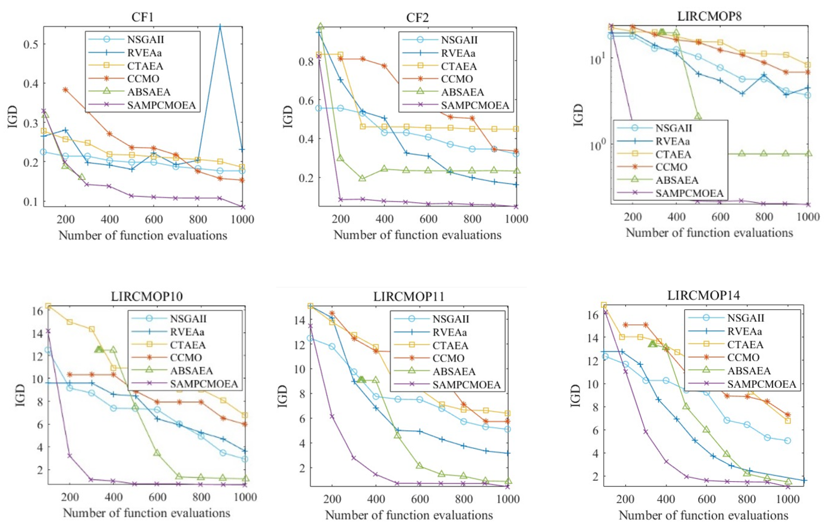
4.1.6. IGD Value Convergence Experiment

In order to demonstrate the convergence curves of the SA-MPCMOEA algorithm compared to other algorithms in terms of the IGD value, we conducted a convergence analysis in CF1, CF2, LIRCMOP8, LIRCMOP10, LIRCMOP11, and LIRCMOP14, respectively. For each test problem, we selected 6 values from 1000 function evaluations to show the convergence variation of the algorithm.

As can be seen in Figure 6, SA-MPCMOEA converges faster than other algorithms when in search mode 1, which demonstrates the effectiveness of the angle-based convergence model. This is mainly because, given limited computational resources, there are fewer individuals available to explore the feasible region. If the algorithm cannot converge quickly to reduce the search range, the population will spend some computational resources on ineffective exploration.

4.1.7. Real-World Case Study

In order to verify the ability of SA-MPCMOEA to solve practical application problems, we conduct verification respectively in RW1 (Pressure Vessel Design), RW2 (Simply Supported I-beam Design), RW3 (Cantilever Beam Design), RW4 (Crash Energy Management for High-speed Trains), and RW5 (Water Resources Management). The mathematical expressions of these five engineering design problems can be found in [35]. In each problem, it is necessary to find the minimum value of different objective functions.

From

Table 8. Performance comparison on RWMOP benchmark problems.

Problem	M	D	NSGA-II	RVEAa	CTAEA	CCMO	ABSAEA	SA-MPCMOEA
RWMOP1	2	4	3.612 × ${10}^{+5}$ (4.93 × ${10}^{+3}$) =	NaN (NaN)	5.998 × ${10}^{+5}$ (4.57 × ${10}^{+5}$) =	3.623 × ${10}^{+5}$ (2.91 × ${10}^{+3}$) =	3.635 × ${10}^{+5}$ (2.78 × ${10}^{+3}$) =	4.392 × ${10}^{+5}$ (1.73 × ${10}^{+5}$)
RWMOP2	2	4	34.92 (33.4) −	220.3 (35.7) −	2.508 (2.08) =	35.56 (33.1) −	35.96 (30.9) −	2.790 (3.06)
RWMOP3	2	2	0.0240 (0.0668) =	1.461 (0.517) −	0.0187 (0.0186) =	0.0240 (0.0668) =	0.7997 (0.583) −	0.0170 (0.0254)
RWMOP4	2	6	1.005 (0.402) −	3.259 (0.468) −	1.181 (0.466) −	1.018 (0.241) −	0.9617 (0.566) −	0.0161 (2.58× ${10}^{-8}$)
RWMOP5	5	3	2.381 × ${10}^{+6}$ (0.072 × ${10}^{+6}$) −	2.530 × ${10}^{+6}$ (0.035 × ${10}^{+6}$) −	2.477 × ${10}^{+6}$ (0.061 × ${10}^{+6}$) −	2.292 × ${10}^{+6}$ (0.126 × ${10}^{+6}$) =	2.359 × ${10}^{+6}$ (0.133 × ${10}^{+6}$) =	2.275 × ${10}^{+6}$ (0.080 × ${10}^{+6}$)
Statistical Summary			0/3/2	0/4/0	0/2/3	0/2/3	0/3/2

, it can be seen that SA-MPCMOEA has achieved the optimal solution or near-optimal solution in all practical engineering problems, demonstrating its applicability in solving practical engineering problems.

5. Conclusions

This paper proposes SA-MPCMOEA, a Kriging-assisted evolutionary algorithm based on a multi-preference model designed to address expensive, constrained multi-objective optimization problems. SA-MPCMOEA dynamically determines subsequent optimization operations by analyzing the current population distribution state. In Mode 1, the algorithm employs an angle-based convergence strategy to rapidly guide the population toward feasible regions using angular distribution information, thereby reducing computational resource waste. Mode 2 enhances convergence performance by driving the main population P and auxiliary population A to approximate the constrained Pareto front and the unconstrained Pareto front, respectively, achieving preference decoupling between objective functions and constraints. Under Mode 3, while maintaining the constraint compliance of population P, the auxiliary population A strengthens exploration capabilities in underdeveloped regions through constraint-free search mechanisms guided by diversity and convergence metrics coupled with hybrid update strategies. Additionally, the dynamic evaluation strategy and novel filling sampling criterion enable effective screening of high-quality candidate solutions, allowing the algorithm to allocate expensive evaluation resources to truly promising individuals. Collectively, SA-MPCMOEA achieves a balanced optimization between objective pursuit and constraint satisfaction in computationally expensive scenarios. The code for SA-MPCMOEA can be found at https://github.com/AMA123-sx/AMA (accessed on 28 March 2025).