Research on Defect Detection of Bare Film in Landfills Based on a Temperature Spectrum Model

Abstract

Due to the construction damage of high-density polyethylene film (HDPE) during the early stages of landfill construction and missed or faulty welding, this paper proposes a method based on the synchronous characteristic temperature differences between defective and intact areas of HDPE film. An image feature-edge-picking algorithm was used to detect various defects. First, under the action of a continuous heat source, infrared images of different types of defects on the surface of HDPE films were collected, and we recorded the temperature of different areas on the film surface. We also analyzed the changes in the temperatures of the complete and defect areas over time and extracted the temperature characteristic curves. Second, the contour characteristics of hidden defects in the weld area were analyzed. The image with the most substantial temperature difference resolution was selected and preliminary noise reduction was performed. Further enhancement of the edges was carried out using the guided image-filtering (GIF) algorithm, which was improved by using the edge-aware weighting in weighted guided image filtering (WGIF) and the weighted aggregation mechanism in weighted aggregated guided image filtering (WAGIF). Finally, the Canny operator was used to detect the edges of the processed images to recognize the contour of the welding defect. The best pixel image was extracted, the pixel comparison relationship was used to quantitatively detect the defect size of the HDPE film and the error between the image defect size and the actual size was analyzed. The experimental results show that the model could identify the surface defects on HDPE film during construction and could obtain the approximate outline and size of the hidden defects in the welding area.

1. Introduction

Currently, rapid economic development speeds up people’s lifestyles and, as a result, the various wastes they generate are increasing [1,2]. As an important destination for waste disposal, landfills also face a severe test [3,4]. Once leakage occurs, they can seriously pollute the surrounding water and soil environment [5]. Therefore, strict standards are required from early-stage design, construction, and testing to later-stage operation monitoring.

Laying an anti-seepage system is one of the important means to hinder diffusion of leachate from landfills. HDPE film is the main anti-seepage material used in landfills [6,7] as it has the advantages of a high anti-seepage coefficient, stable chemical performance, high mechanical strength, long life, and low cost [8].

In the early stages of landfill anti-seepage systems construction, there are two main causes of surface damage to the HDPE film. First, irregular defects on the HDPE film surface can be caused by construction machinery and personnel activities. Second, during the welding of the HDPE film, incorrect welding operation and improper material selection can cause hole defects, missed or faulty welding, and uneven fusion between films. In addition, excessive welding pressure can cause welding seam fractures. The defects in HDPE film caused by these damage factors can cause potential safety hazards in the operation stage of the landfill [9,10].

Methods for evaluating HDPE film defects during the construction stage are mainly divided into destructive [11] and nondestructive assessments. Destructive assessment involves testing the strength of geomembrane samples from the welding area through shear or tensile tests. The test results can be used to guide and set the relevant welding form and parameters, but the detection process may cause secondary damage to the HDPE. Nondestructive assessment is mainly achieved using an electrical method [12,13] or an ultrasound testing method [14]. The electrical method involves installing electrodes beneath the HDPE film and applying a high-voltage power source above the film. When holes or defects exist, detectable current pathways are formed, enabling the identification of damaged locations. However, this electrical detection system features complex architecture and requires preinstalled electrodes, which significantly increases construction costs for landfill sites. The ultrasonic detection method is based on the characteristics of ultrasonic Lamb wave scattering through the damage point, resulting in energy attenuation. The method uses wavelet analysis to define the damage index and, combined with damage imaging, identifies the location of the leakage in the HDPE film. However, the Lamb wave signal is very easy to lose in the background noise. In addition, the method cannot effectively detect defects within the weld seam [15].

Compared with other methods, infrared thermal imaging inspection technology has the advantages of intuitive and easy-to-understand images, fast detection speed, and low cost; it can also achieve efficient and reliable detection of small defects. It has been widely used in the field of nondestructive testing [16,17]. In wastewater treatment plants, defects in HDPE films can be detected by analyzing cloud-induced temperature changes on the film surface. This method requires that the cloud cover lasts for more than 1 min and that the solar radiation drops by more than 400 W/m². However, the duration of cloud cover is unpredictable in natural environments. This unpredictability limits the practical application of this method [18].

In this study, infrared technology was used to detect welding defects on the surface of HDPE film and inside the weld seam based on the characteristics of the simultaneous temperature difference between the defective area and the intact area of HDPE film in a landfill. HDPE film defect edges contain much information [19,20,21], and extracting the defect edges from infrared images can effectively identify the geometric features of the defects. Based on improved guided image filtering and edge detection image processing to solve the problem of measuring the internal defect size of the HDPE film weld seam, a completely different method was used to locate the defect area in the infrared image of the HDPE film.

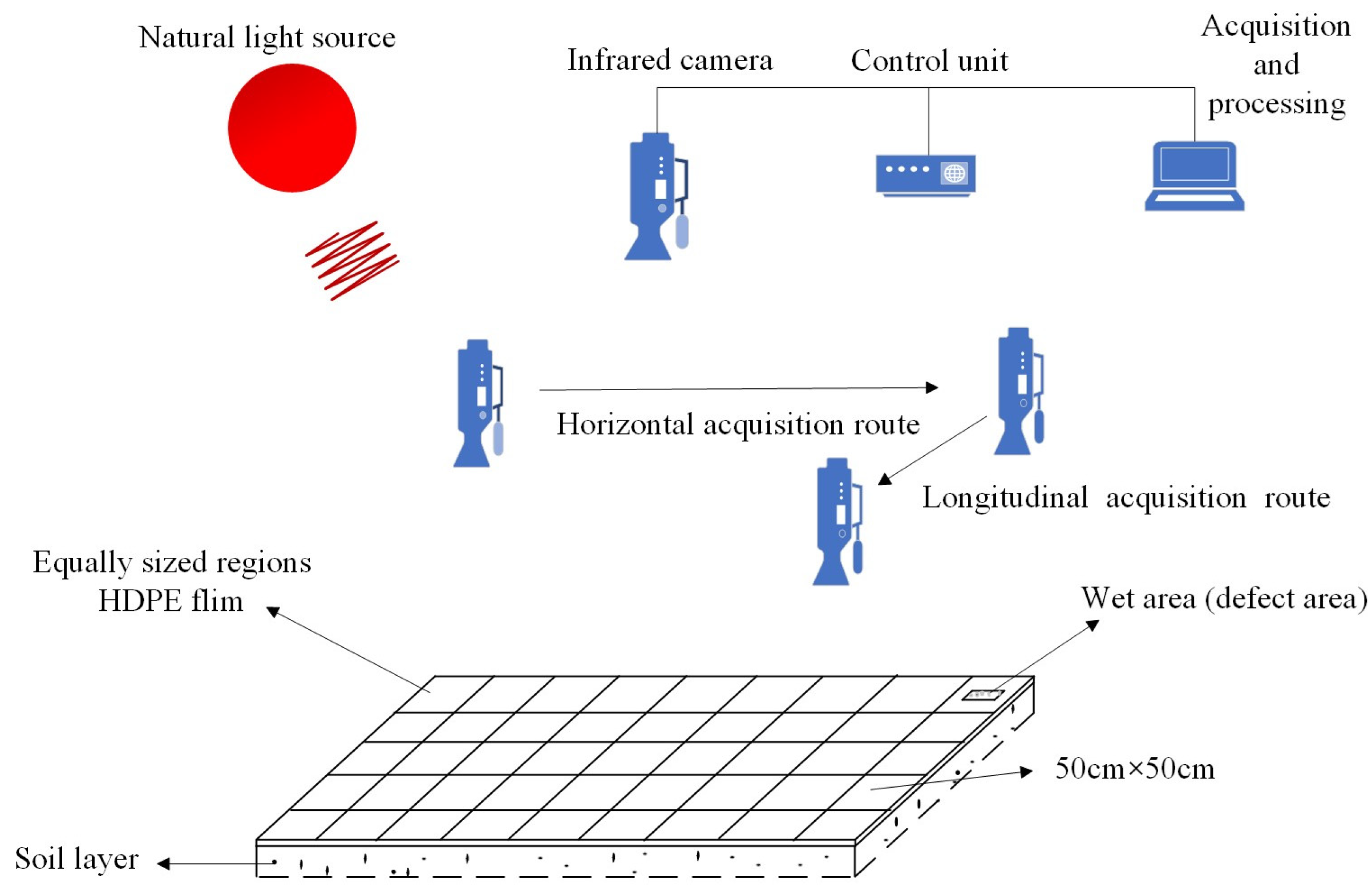
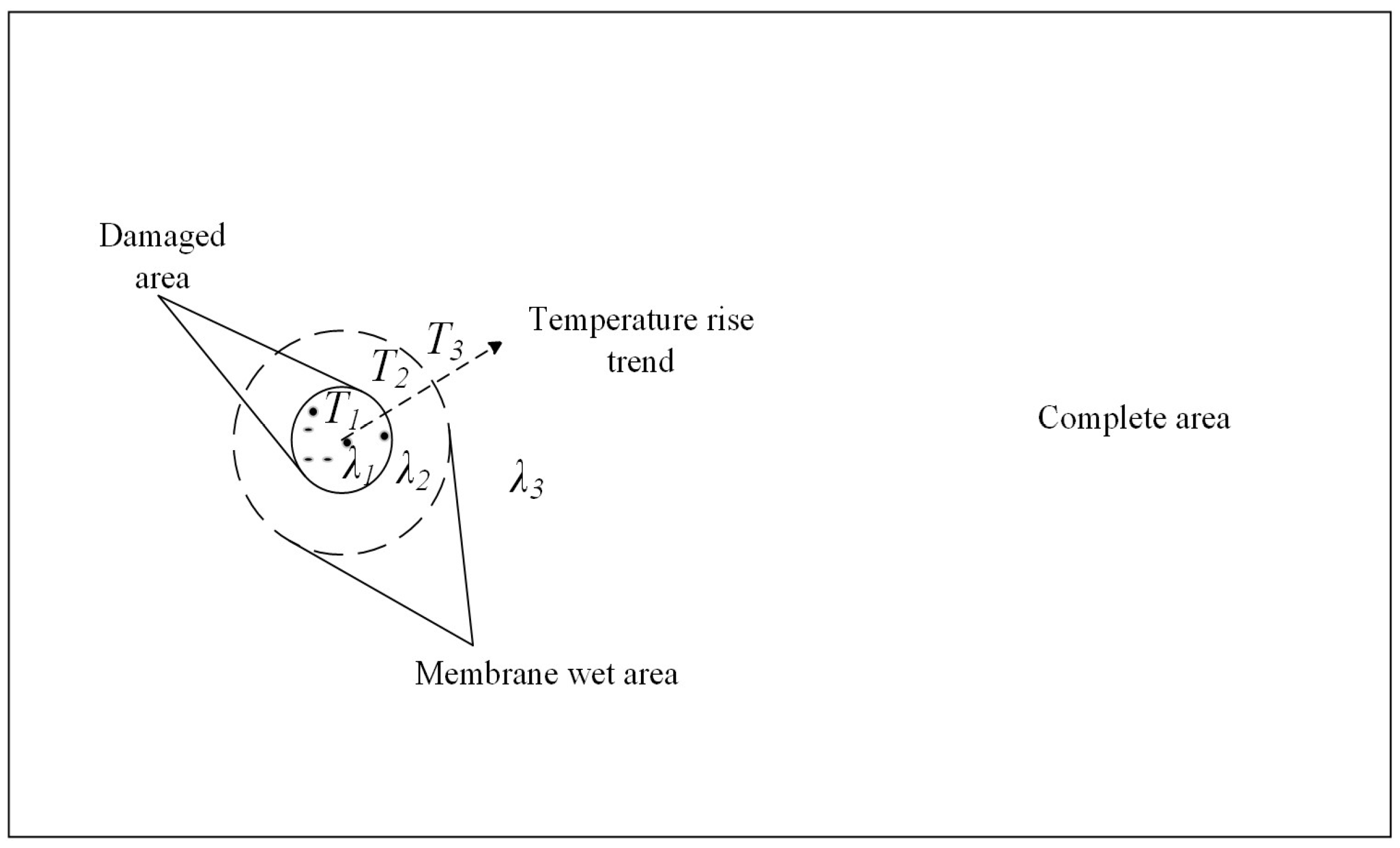
2. Position Detection Principle

The detection principle of bare film defects under a natural light source based on a heat conduction model is as follows: under conditions where natural heat sources are sufficient (as shown in Figure 1, where the sun serves as the natural heat source) and the minimum ambient temperature is 37 °C, the HDPE film after 30 min of exposure is laid over the soil layer and the HDPE film is cooled by sprinkling water (the water temperature was generally maintained at 20–25 °C). Due to the thermal diffusion coefficient of the wet soil layer, below the defect area is different from the unruptured area of the HDPE film. Defective and complete areas will have synchronized temperature difference characteristics, and the location of the defective areas can be identified from the captured infrared images. In the detection process, given the extensive coverage of HDPE films in landfill installations, the HDPE film was divided into equally sized areas (area size is 50 cm × 50 cm) and the surface of a specific area cooled through water flow. An infrared thermal imaging camera was used to capture infrared images of this area until no temperature difference was detected. The above operation was carried out on the entire surface of the HDPE film by means of preset horizontal and longitudinal acquisition routes. The detection principle is shown in Figure 1.

Infrared heat waves follow the heat conduction equation as they propagate through the HDPE film. To detect defects, only heat conduction in the depth direction is considered. When the thermal conductivity is determined, the heat conduction equation is:

$$\nabla \cdot \left[k\nabla T(x,t)\right]-\rho c{\displaystyle \frac{\partial T(x,t)}{\partial t}}=-f(x,t)$$

(1)

For the plane heat source available:

$$f(x,t)=q\delta (x)\delta (t)$$

(2)

Bringing Equation (2) into Equation (1) yields:

$$\left\{\begin{array}{c}{\displaystyle \frac{{\partial }^{2}T(x,t)}{\partial x^2}}-{\displaystyle \frac{1}{\alpha }}{\displaystyle \frac{\partial T(x,t)}{\partial t}}=-{\displaystyle \frac{q}{\lambda }}\delta (x)\delta (t)\\ \alpha =\lambda /\rho c\end{array}\right.$$

(3)

In Formula (3), $x$ is the position in the depth direction, $t$ is the time, $T$ is the temperature, $\alpha$ is the thermal diffusion coefficient of the medium, and $\lambda$ is the thermal conductivity, where ${\lambda }_1$ is the thermal conductivity of moist soil in the broken area; ${\lambda }_2$ is the equivalent thermal conductivity of the area under the joint influence of the HDPE membrane and moist soil; and ${\lambda }_3$ is the thermal conductivity of the unbroken area of the HDPE membrane. $\rho$ is the density, $c$ is the specific heat capacity, and $q$ is heat flux density. When the value of $\lambda$ is larger, the object reacts faster to the change in ambient temperature. The moist soil in the defect area acts as a heat-conducting medium, which has the largest thermal conductivity ${\lambda }_1$ and the fastest response to environmental temperature changes. The humid area under the film is affected by the HDPE and the humid soil, and its equivalent ${\lambda }_2$ value is less than ${\lambda }_1$ and greater than ${\lambda }_3$. Therefore, within a period of time after the sprinkling water cools down, the temperature rise trend is $T_1<T_2<T_3$, as shown in Figure 2.

The relative thermal value is approximated as the difference between the surface temperature of the complete area of the HDPE film ($T_3$) and the defective area ($T_1$), expressed by $\Delta T$ as:

$$\Delta T=T_3-T_1$$

(4)

By analyzing the above formulas, we know that, due to the effect of water flow, when the HDPE film has defects, it will cause fluctuations in the thermal field on the surface of the film, which ultimately affects the infrared radiation detection process.

3. Defect Detection Experiment

3.1. Experimental Materials and Performance Parameters

An infrared thermal imager (Fluke Tis10 9 Hz Thermal Imager, Fluke, Everett, WA, USA) was used; accuracy is ±2 °C, the working temperature is −10 to +50 °C, resolution is 80 × 60, and the infrared thermal imager working band is 7.5–14 μm to meet accuracy claim. HDPE film thickness is 0.15 cm and 0.20 cm, with an emissivity of 0.93 and a transmittance of less than 5%, puncture strength is 249 N, fracture strength is 53 N, thermal conductivity is 0.527 W/(m·k), and the average thermal conductivity of the wet soil layer is 1.052 W/(m·k).

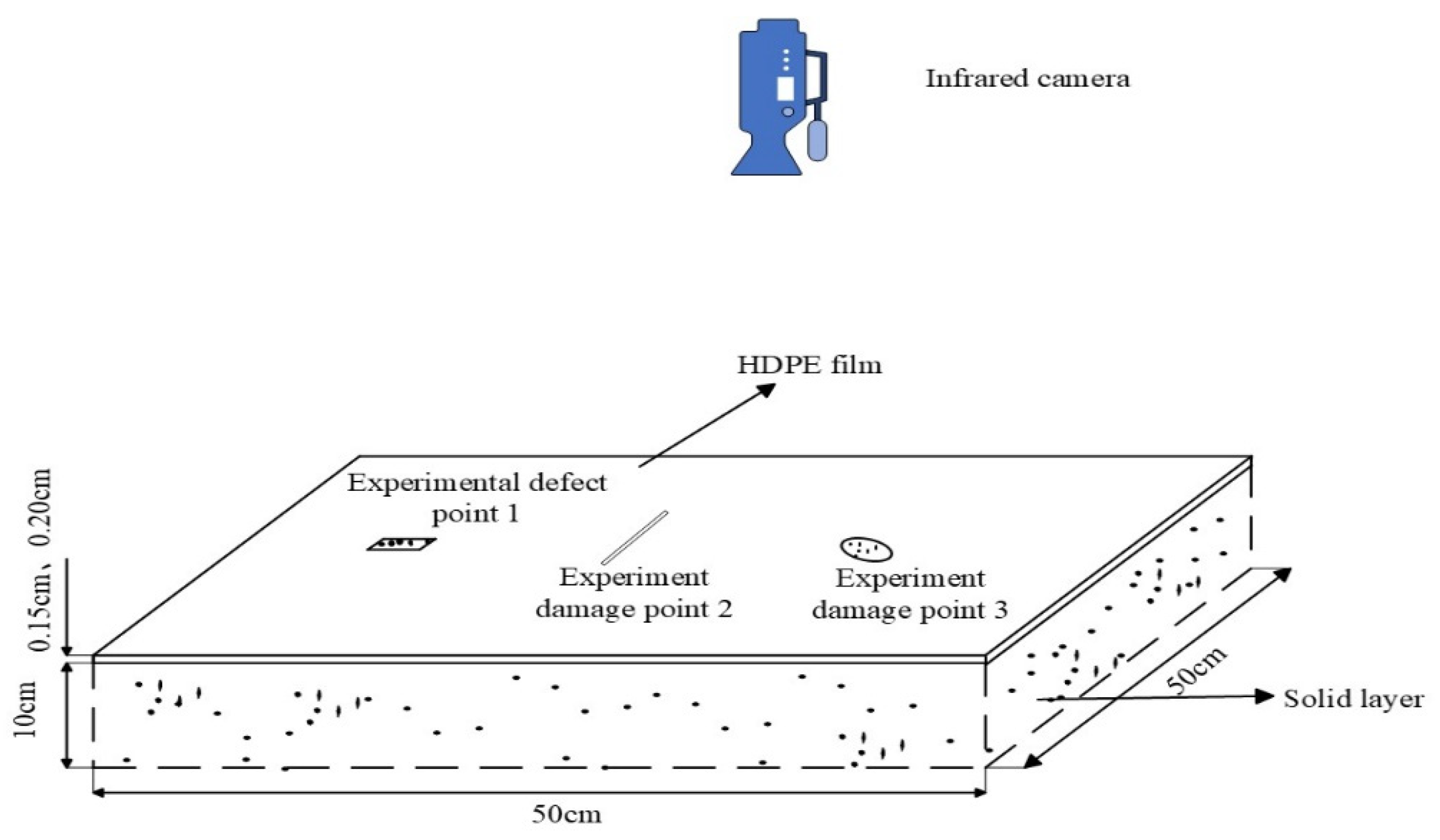
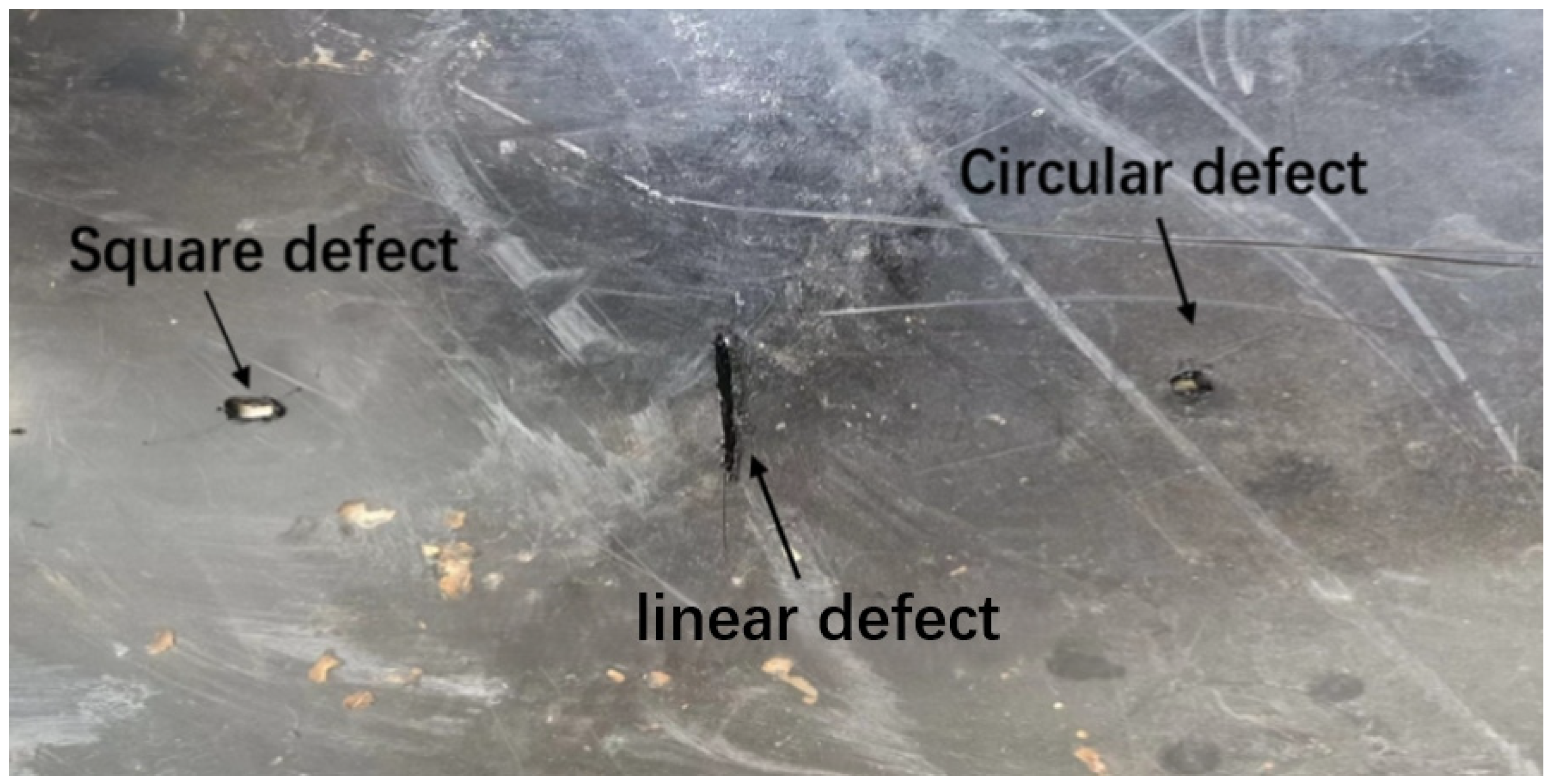
3.2. Test Sample Preparation

All experimental designs, sample preparations, and data collections in this study were independently completed by the authors’ research team. We made an experimental soil box with a size of 50 × 50 × 20 cm, laid HDPE film on the top layer; a natural soil layer with a thickness of 10 cm was laid under the film, as shown in Figure 3. We set defects of different shapes on the surface of HDPE film, and the number of the defect area is 1, 2, and 3; number 1 is a square defect, number 2 is a linear defect, and number 3 is a circular defect, as shown in Figure 4. Detection tests were carried out on HDPE films (thicknesses of 0.15 cm and 0.20 cm) according to the detection principle.

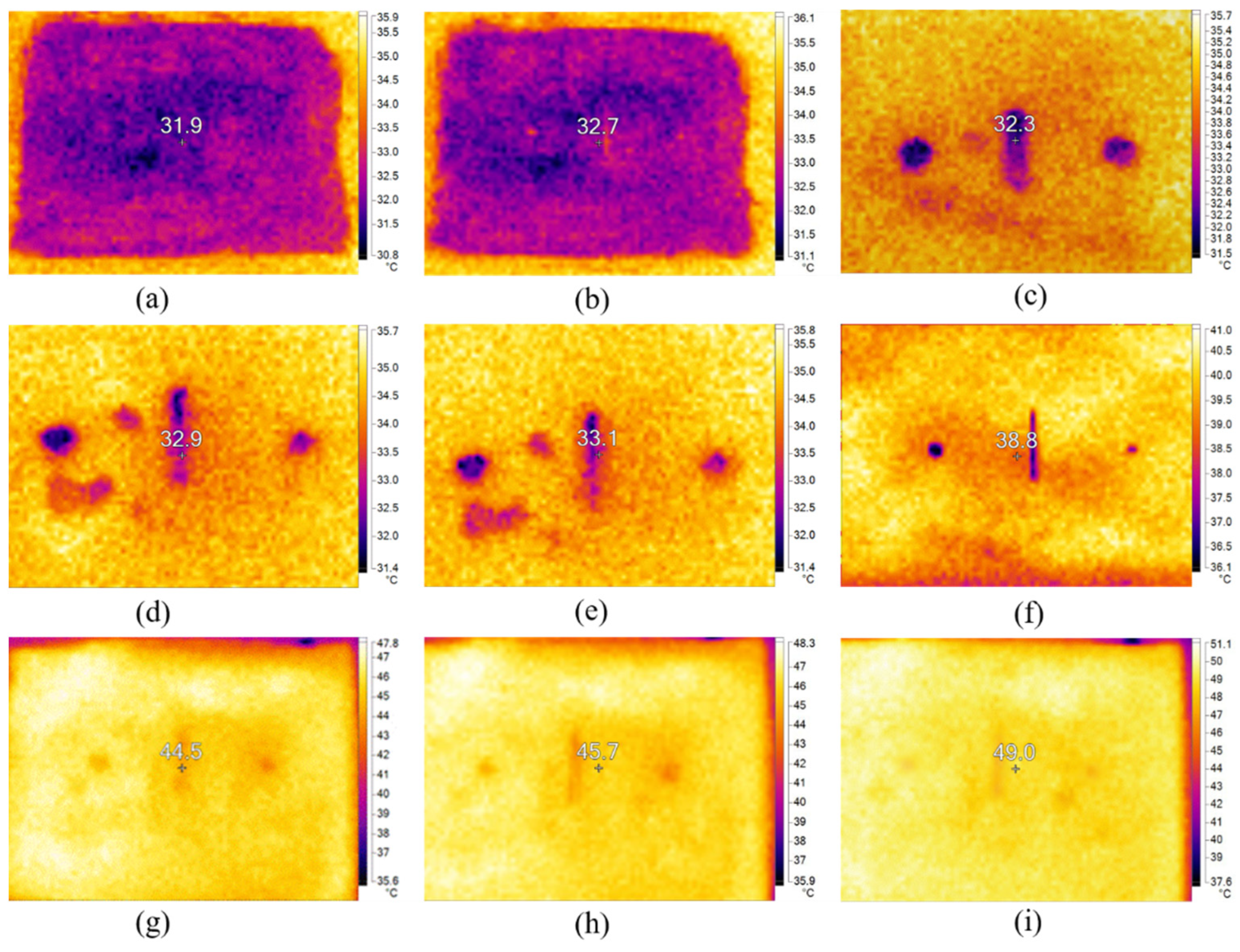
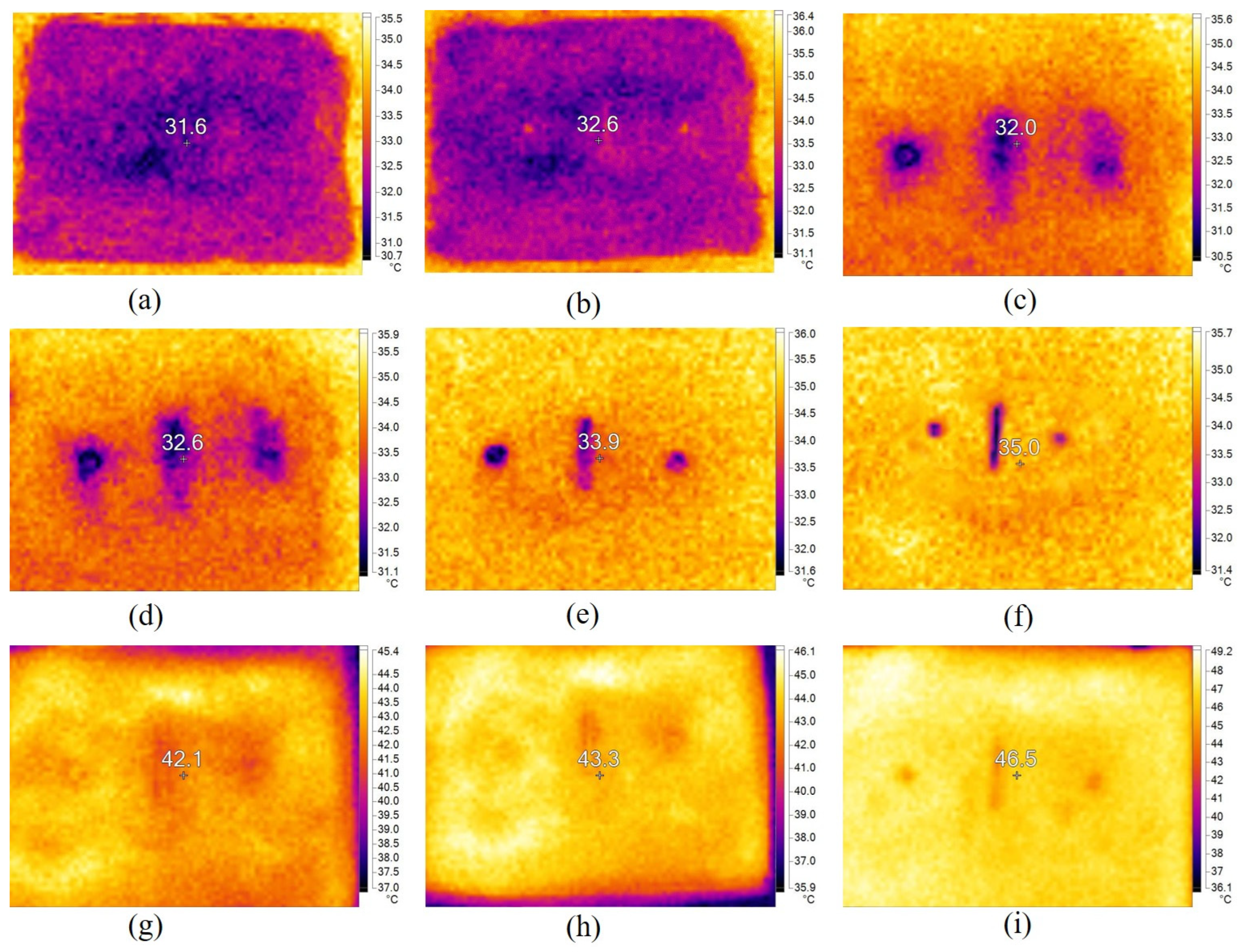
3.3. Test Analysis of Different Thicknesses of HDPE Film

Infrared images of 0.15 cm HDPE film at different heating times are shown in Figure 5; t = 0.0 min means that the HDPE film has just cooled by water flow and the overall temperature of the film surface has dropped. Starting from t = 0.5 min, the defect and complete area begin to show temperature difference characteristics. In the initial cooling stage, the direct contact area of the water flow with the HDPE film complete area is greater than the defect area soil layer, resulting in a decrease in the temperature drop rate of the defect area. Therefore, in Figure 5b, the temperature of the defect area is too high. At t = 10.0 min, the temperature in the complete area is considerably higher than the temperature around the defect area. Due to the convection effect of the heat source and the soil layer in the defect area and the thermal conductivity of the soil layer being greater than the HDPE film, the temperature around the defect area is lower. As shown in Figure 5c, after t = 11 min, under the continuous natural heat source, the temperature around the defect area gradually rises and the defect contour in the infrared image continues to decrease, as shown in Figure 5d–f. Interference areas exist below the square defect and between the square defect and linear defects in Figure 5d,e. This is caused by uneven sprinkling leading to slower temperature rise in interference areas; these areas do not exhibit the purple low-temperature characteristics observed at defects under the same time conditions. The heat capacity is saturated in the t = 20–25 min time period; the temperature of the defective area is similar to that of the intact area, and the infrared edge contour gradually disappears, as shown in Figure 5g–i.

Infrared images of 0.20 cm HDPE film at different heating times are shown in Figure 6. Compared with Figure 5, it can be seen that the defect profile change time of the two HDPE films with different thicknesses is about the same under the condition of sufficient natural heat source, but the defect contour of the 0.20 cm thick HDPE film is blurred at the same time, as shown in Figure 6c–f. The 0.20 cm thick HDPE film, being relatively thick and having a high heat capacity, continues to absorb heat and increase in temperature at t = 20 min. Additionally, there are minor differences in the heating rates across the film’s surface. This causes the defect contours initially formed by temperature differences in the infrared images to gradually blur, as shown in Figure 6g. As the temperature increases, the heat capacity of the HDPE film approaches saturation, leading to a reduction in regional temperature differences. By t = 25 min, the temperature difference between the defective and intact areas becomes similar and the infrared edge contours almost disappear, as shown in Figure 6i.

To further analyze the HDPE film defect status, the temperature data of the defect area and the intact area at different times in Figure 5 and Figure 6 were extracted, as shown in

Table 1. Temperature difference data at different times in the 0.15 cm HDPE film defective–complete area.

Time/min	Defect Areas Average Temperature/°C	Complete Area Average Temperature/°C	Temperature Difference/°C
0	32.6	31.9	0.7
10	31.6	34.8	−3.2
11	32.5	35.6	−3.1
12	33.1	36.5	−3.4
13	33.7	37.5	−3.8
20	44.4	46.3	−1.9
25	47.3	49.0	−1.7

and

Table 2. Temperature difference data at different times in the 0.20 cm HDPE film defective–complete area.

Time/min	Defect Areas Average Temperature/°C	Complete Area Average Temperature/°C	Temperature Difference/°C
0	32.3	31.7	0.6
10	31.4	33.4	−2
11	31.7	34.1	−2.4
12	32.3	34.9	−2.6
13	32.8	35.4	−2.6
20	40.8	42.7	−1.9
25	45.5	46.5	−1.0

, and temperature curves were plotted for analysis. The surface temperature curve of the defective and intact area for Figure 5 is shown in Figure 7 and the surface temperature curve of the defective and intact area for Figure 6 is shown in Figure 8; from Figure 7 and Figure 8, it can be seen that, in the same role of the environment, the two thicknesses of HDPE film defective area and intact area have a similar temperature trend; HDPE film with a thickness of 0.15 cm has a large relative temperature difference value for a period of 10–20 min. It can be seen in Table 1 that, when t = 13 min, the temperature difference is the largest, and the observed results are more obvious. As the film thickness increases, the thermal capacity increases. The HDPE film with a thickness of 0.20 cm takes longer to rise to the same temperature, while the thermal conductivity of the area of the defect does not change significantly. Therefore, the slower rise in temperature of the HDPE film with a thickness of 0.20 cm results in a later and blurrier appearance of the defect contour, and shrinkage occurs during the time period when the temperature difference characteristic is most significant. The time period with larger values of relative temperature difference is 11–18 min, and the largest value of temperature difference between the defective and intact areas is observed at t = 14 min, where the results are more pronounced.

4. HDPE Film Weld Defect Detection Test

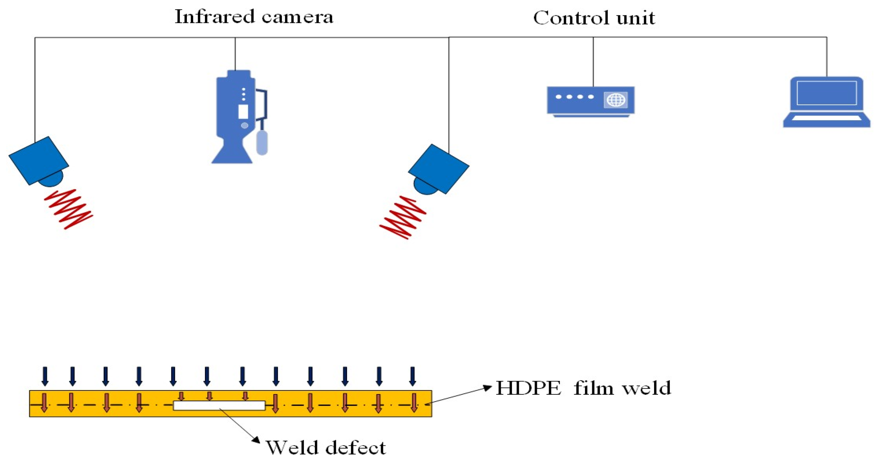
4.1. Improvement of Test Device

Considering the concealment of the defect location at the welding seam, the water flow cooling method cannot identify the edge of the weld contour, which affects the final repair process. Thus, for the defect of the welding seam, the experimental setup needs to be improved. The infrared thermal imaging system device used to detect defects at the welding seam of the HDPE film is shown in Figure 9. The device is composed of two 500 W halogen lamp heating sources, an infrared thermal imager, and a terminal computer. The HDPE film material was heated by a heating source, and an infrared image of the material was collected by a Fluke Tis10 9 Hz thermal imager. The heating source and the infrared thermal imager are fixed at a certain distance from the HDPE film, while ensuring that the infrared thermal imager is perpendicular to the surface of the HDPE film. This setup not only enables sufficient heating of the material but also facilitates full-coverage image acquisition by the infrared thermal imager. Improving the GIF is used to reduce the small noise interference of the image and retain the defect contour [22,23]. Combined with the edge contour extraction technique, important information about the defective area of the rendered image is extracted to establish an infrared thermal imaging system for defect detection of HDPE film.

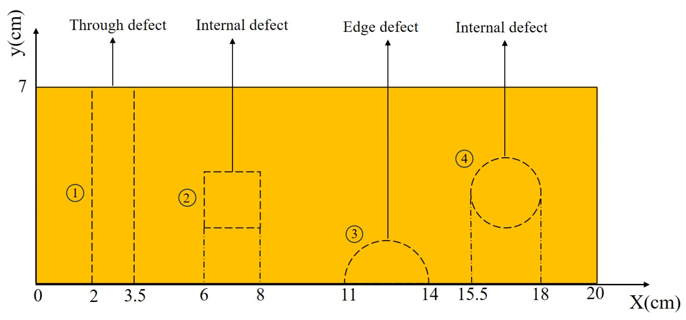
4.2. Preparation of Test Samples

Preparing defects at weld seams of HDPE film, as shown in Figure 10, the number 1 is a through defect and represents the position of the missing welding under actual working conditions. The numbers 2 and 4 are internal defects of the welding seam, and the number 3 is the edge defect. Number 2, number 3, and number 4 represent different types of virtual welding under actual working conditions. Number 1 is a rectangle 7.0 cm long and 1.5 cm wide, number 2 is a square with a side length of 2 cm, number 3 is a semicircle with a radius of 1.75 cm, and number 4 is a circle with a radius of 1.25 cm. After the test began, under the heating effect of the halogen lamp, the infrared thermal imager continuously captured infrared images of the weld area of the HDPE film.

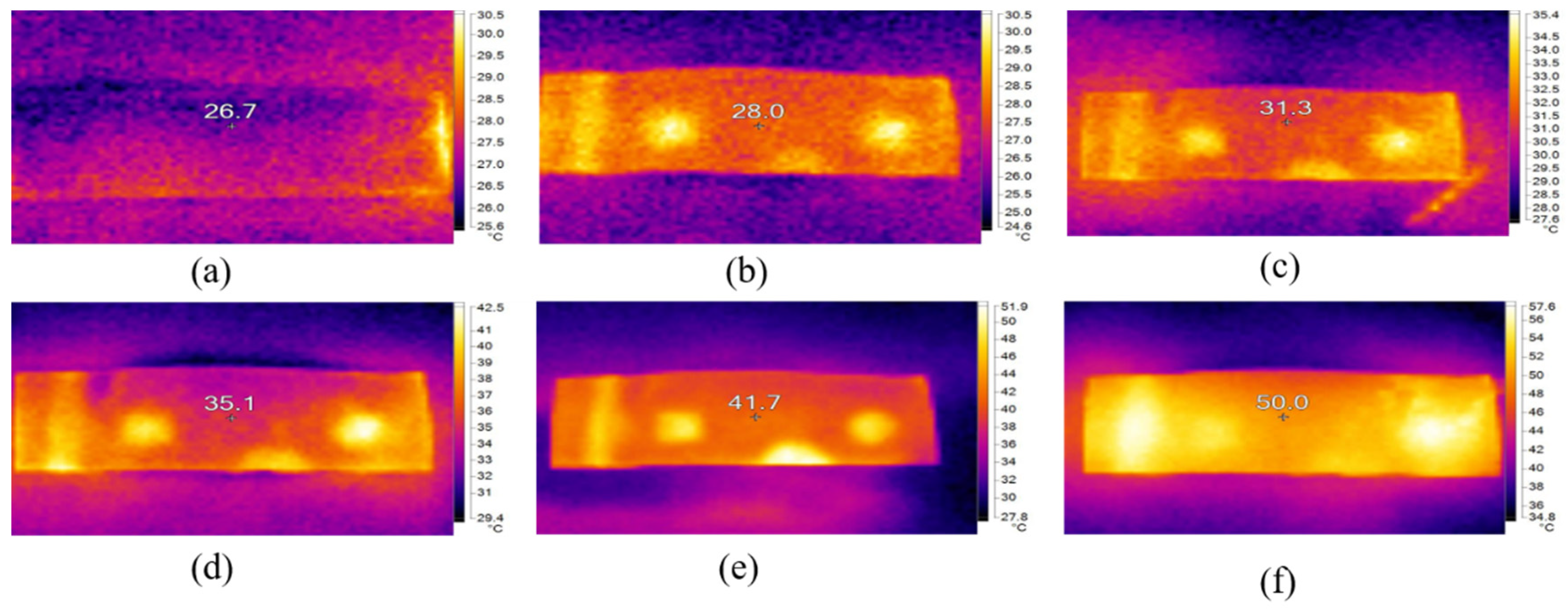
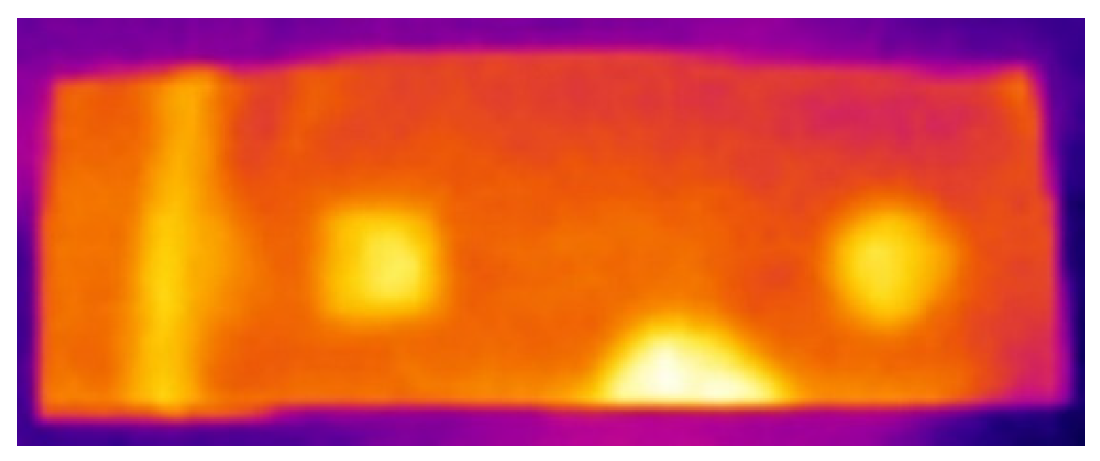
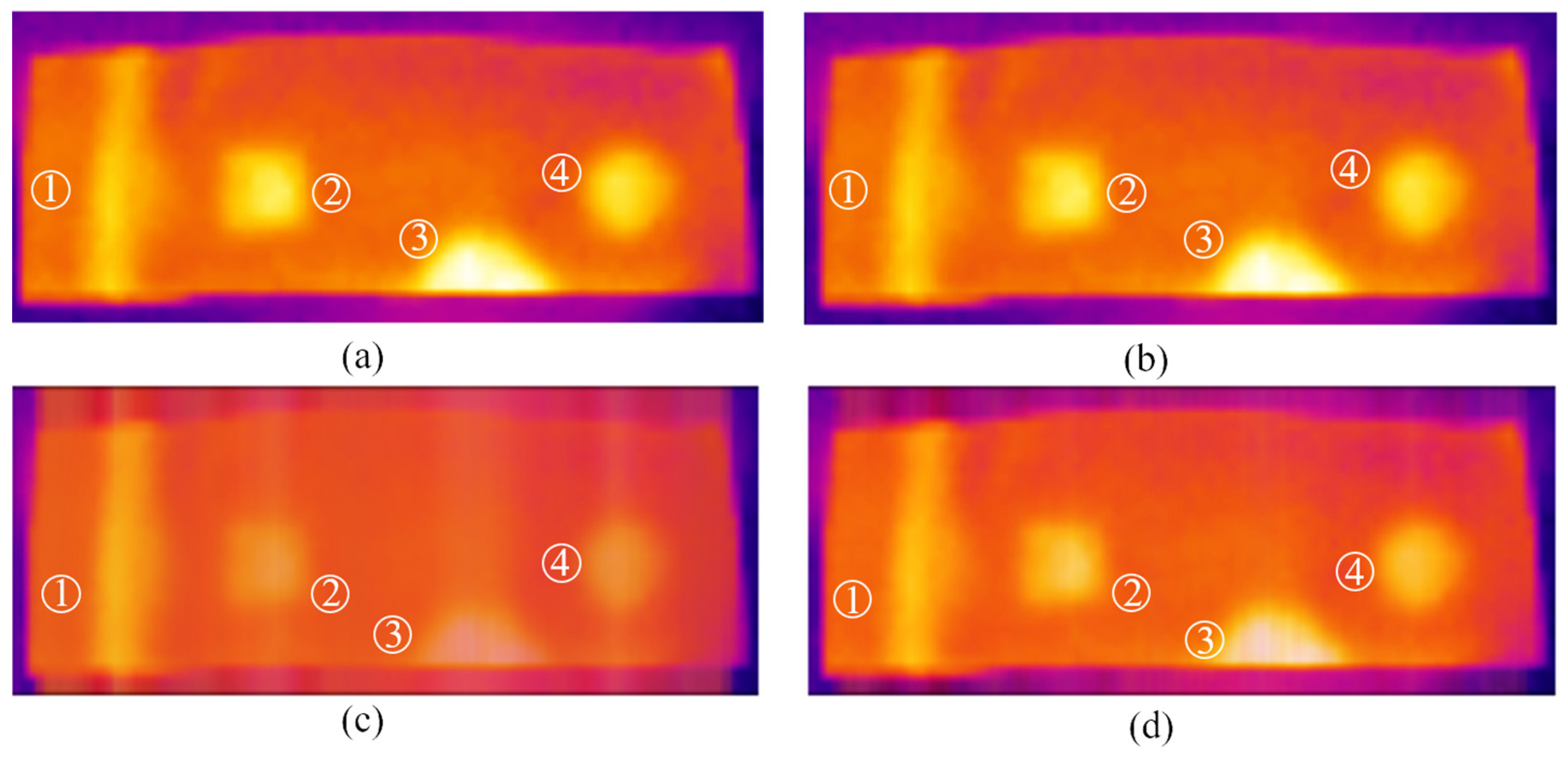
4.3. Analysis of Weld Defect Test Results

The infrared images of the HDPE weld at different heating time intervals are shown in Figure 11. From these images, it can be seen that, due to the poor welding quality in the defect area, the heat from the upper HDPE film cannot dissipate to the lower HDPE film. This causes the defect area to heat up more quickly within the same time period, creating a temperature difference compared to the intact area, as shown in Figure 11a–e. As the heating time continues to increase, heat is transferred from the higher-temperature defect area to the lower-temperature intact area through heat conduction, causing the edges of the defect area to become blurred, as shown in Figure 11f.

The temperature data of the defect area and the intact area at different times from Figure 11 are extracted as shown in

Table 3. Temperature difference data at different times in the weld defective–complete area.

Time/min	Defect Areas Average Temperature/°C	Complete Area Average Temperature/°C	Temperature Difference/°C
0	26.6	26.6	0
1	30.1	28.1	2
2	33.9	31.1	2.8
3	40.7	35.6	5.1
4	49.8	41.7	8.1
5	58.7	50.8	7.9

, and a temperature curve is plotted, as seen in Figure 12. From the temperature curve, it is evident that the temperature difference between the defect area and the intact area of the HDPE film is significant during the 3–5 min interval. This period can be considered the optimal time frame for detection.

5. Image Analysis

The entire HDPE film defect identification process is divided into three stages. The first stage is the preprocessing of the image, which is used to improve the image quality, and the image is preprocessed by using the improved guided filtering technology so as to minimize the misidentification rate of image defects and optimize the edge effect of the defects. The second stage is a series of edge contour recognition methods for infrared images, which use Canny, Sobel, Prewitt, and Roberts edge detection algorithms to identify and process the edge information in infrared images. The contour of the defect is determined. The third stage is pixel analysis, which uses pixel analysis to calculate the defect length.

5.1. Preprocessing Algorithm

Based on the difference between the adjacent pixel values in the infrared image window of the HDPE film, the weight is given to smooth the image. The guide filter function satisfies the linear relationship in the two-dimensional window of the infrared image as [24,25,26]:

$$q_i=a_k{I}_i+b_k,{\forall }_i\in w_k$$

(5)

In Formula (5), $q$ represents the pixel value of the output image, $I$ represents the guidance image, $i$ and $k$ represent the pixel index, and the two coefficients $a_k$ and $b_k$ are jointly determined according to the input image $p$ and the guidance image $I$. $w_k$ is a local window centered on pixel $k$. The gradient can be obtained by solving both sides of Equation (5):

$$\nabla q_i=a_k\nabla I_i$$

(6)

Solving for the coefficients of the linear function requires the construction of a minimization cost constraint function, denoted as:

$$E(a_k,b_k)={\displaystyle \sum _{i\in w_k}({(a_k{I}_i+b_k-p_i)}^2+\epsilon {a_k}^2)}$$

(7)

In Equation (7), $\epsilon$ is an important parameter that affects the filtering effect.

$$\begin{array}{c}{a}_k={\displaystyle \frac{\frac{1}{\left|w\right|}{\displaystyle \sum _{i\in w_k}{I}_i{p}_i-{\mu }_k{\stackrel{-}{p}}_k}}{{{\sigma }_k}^2+\epsilon }}\\ b_k={\stackrel{-}{p}}_k-a_k{\mu }_k\end{array}$$

(8)

In Equation (8), $\left|w\right|$ is the total pixels in the window, ${{\sigma }_k}^2$ is the variance of $I$ in window $w_k$, ${\mu }_k$ is the mean value of $I$ in window $w_k$, and ${\stackrel{-}{p}}_k$ is the mean value of the input image $p$.

When the input image is a bootstrap image, the linear regression algorithm is used to find $a_k$ and $b_k$, which can be obtained as:

$$\begin{array}{c}{a}_k={\displaystyle \frac{{{\sigma }_k}^2}{{{\sigma }_k}^2+\epsilon }}\\ b_k=(1-a_k){\mu }_k\end{array}$$

(9)

From Equation (9), it can be concluded that, when the filter window is located in a flat region, ${{\sigma }_k}^2$ is smaller, so that the $a_k$ value tends to 0 and so that the $b_k$ value will be close to the average value of the window ${\mu }_k$; at this time, the bootstrap filtering approximates the mean value of the filter and, when the filter window is in the edge area where the grey level of the image varies greatly, the ${{\sigma }_k}^2$ value is larger, the $a_k$ value is approximated to 1, and the $b_k$ tends to 0. At this time, the filtering effect is very weak. The filtering output value and the gray value of the original image are approximately equal, which protects the edge information of the image. When it comes to the calculation of the window’s linear coefficients, a single pixel will be encompassed by multiple windows. So, it is necessary to average the value of the linear function that encompasses the point, and its output can be expressed as:

$$q_i={\displaystyle \frac{1}{\left|w\right|}}{\displaystyle \sum _{k:i\in w_k}(a_k{I}_i+b_k)={\stackrel{-}{a}}_i{I}_i+{\stackrel{-}{b}}_i}$$

(10)

In Equation (10), $\overline{a_i}={\displaystyle \frac{1}{\left|w\right|}}{\displaystyle \sum _{k\in w_k}{a}_k}$ and $\overline{b_i}={\displaystyle \frac{1}{\left|w\right|}}{\displaystyle \sum _{k\in w_k}{b}_k}$.

5.2. Improved Guided Image Filtering

The smoothing coefficients $\epsilon$ for different regions of the image are adjusted by introducing the edge-aware weights from WGIF [27]; the formula for $a_k$ becomes:

$$a_k={\displaystyle \frac{{{\sigma }^2}_k}{{{\sigma }^2}_k+\epsilon /\zeta (k)}}$$

(11)

Among them:

$$\zeta (i)={\displaystyle \frac{1}{N}}{\displaystyle \sum _{i^{\prime }=1}^N\frac{{{\sigma }^2}_{I,i}(i)+\rho \prime }{{{\sigma }^2}_{I,i}(i\prime )+\rho \prime }}$$

(12)

In Equation (12), ${{\sigma }^2}_{I,i}(i)$ is the variance of the $3\times 3$ window centered on pixel $i$ in $I$, $N$ is the number of pixels, $i\prime$ is used to traverse the variance of all the windows, and $\rho \prime$ is a very small number that prevents $\zeta (i)$ and the denominator from being 0.

The weighted aggregation mechanism is introduced in WAGIF [28]. The GIF obtains the filtered pixel values by calculating the weighted average of the pixels within a local window, and averaging when the edge points are on the same and different sides of the window will weaken the edges; thus, the mean square error is proposed as an exponential mapping for the allocation of the local window of the new aggregated weights, which can greatly minimize the appearance of halos with the expression:

$$\begin{array}{c}{e}_k={\displaystyle \frac{1}{N}}{{\displaystyle \sum _{i\in w_k}(a_k{I}_i+b_k-I_i)}}^2\\ r_k=\exp (-{\displaystyle \frac{e_k}{\eta }})\\ q_i={\displaystyle \frac{1}{\left|r_k\right|}}{\displaystyle \sum _{k,i\in w_k}{r}_k(a_k{I}_i+b_k)}\end{array}$$

(13)

In Equation (13), $e_k$ is the mean square error; $\eta$ is a constant less than 1; $r_k$ is the weight of window $w_k$; and $\left|r_k\right|={\displaystyle \sum _{k\in w_k}{r}_k}$ is a normalization coefficient. This algorithm preserves the edge information of the signal better compared to the original mean aggregation method.

In order to extract better detail information, this paper will introduce both the weighted aggregation mechanism in WAGIF and WGIF improved edge-aware weights to improve the GIF algorithm. The specific formulas are as follows:

$$\begin{array}{l}{a}_k={\displaystyle \frac{{{\sigma }^2}_k}{{{\sigma }^2}_k+\epsilon /\zeta (i)}}\\ \psi {\prime }_k=\exp (-{\displaystyle \frac{{\sigma }_k^2}{{{\sigma }^2}_{I,i}(i)}})\\ q_i={\displaystyle \frac{1}{\left|\psi {\prime }_k\right|}}{\displaystyle \sum _{k,i\in w_k}\psi {\prime }_k(a_k{I}_i+b_k)}\end{array}$$

(14)

In Equation (14), $\psi {\prime }_k$ represents the new aggregation weight factor; when the pixel is located in the edge region, the perceived weight factor $\zeta (i)$ becomes larger and $\epsilon /\zeta (i)$ becomes smaller, and the algorithm realizes the edge-preserving effect. At the same time, the aggregation weight of the window should be smaller and the edge protection is better.

Figure 13 shows the input original image, Figure 14 shows the results after processing by different algorithms, Figure 14a shows the output of bootstrap filtering, Figure 14b shows the output of weighted bootstrap filtering, Figure 14c shows the output of weighted aggregated bootstrap image filtering, and Figure 14d shows the output of the improved guided filtering. The four image-filtering techniques can smooth the image while preserving edges, rather than enhancing contrast. Therefore, compared to the original image, their outputs show almost no noticeable difference. However, significant differences will appear when edge detection is applied.

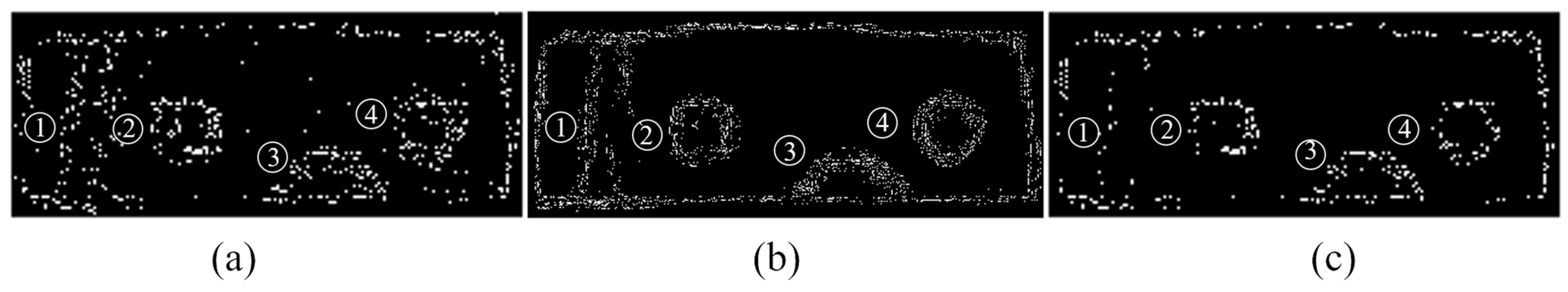
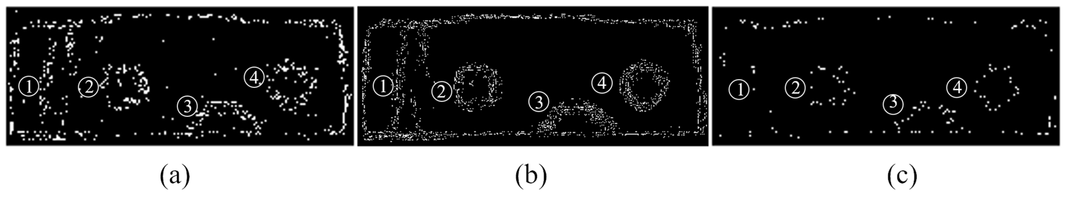
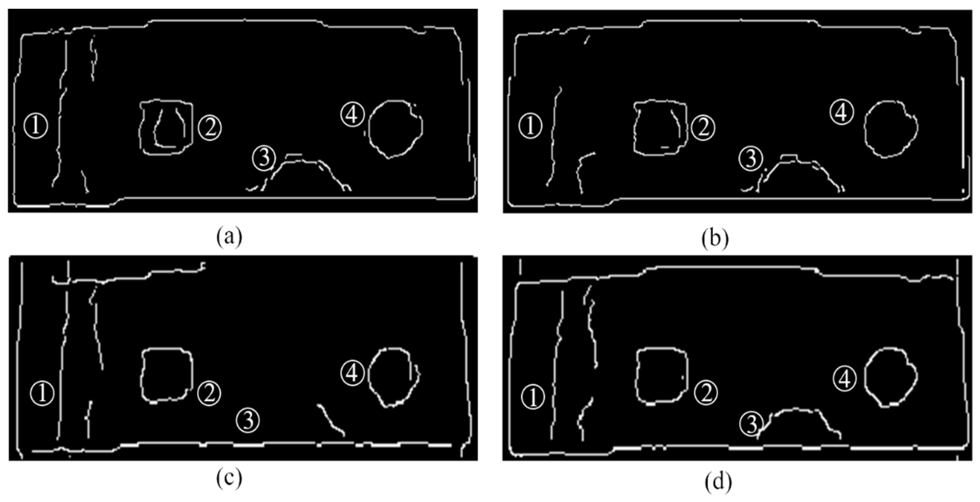
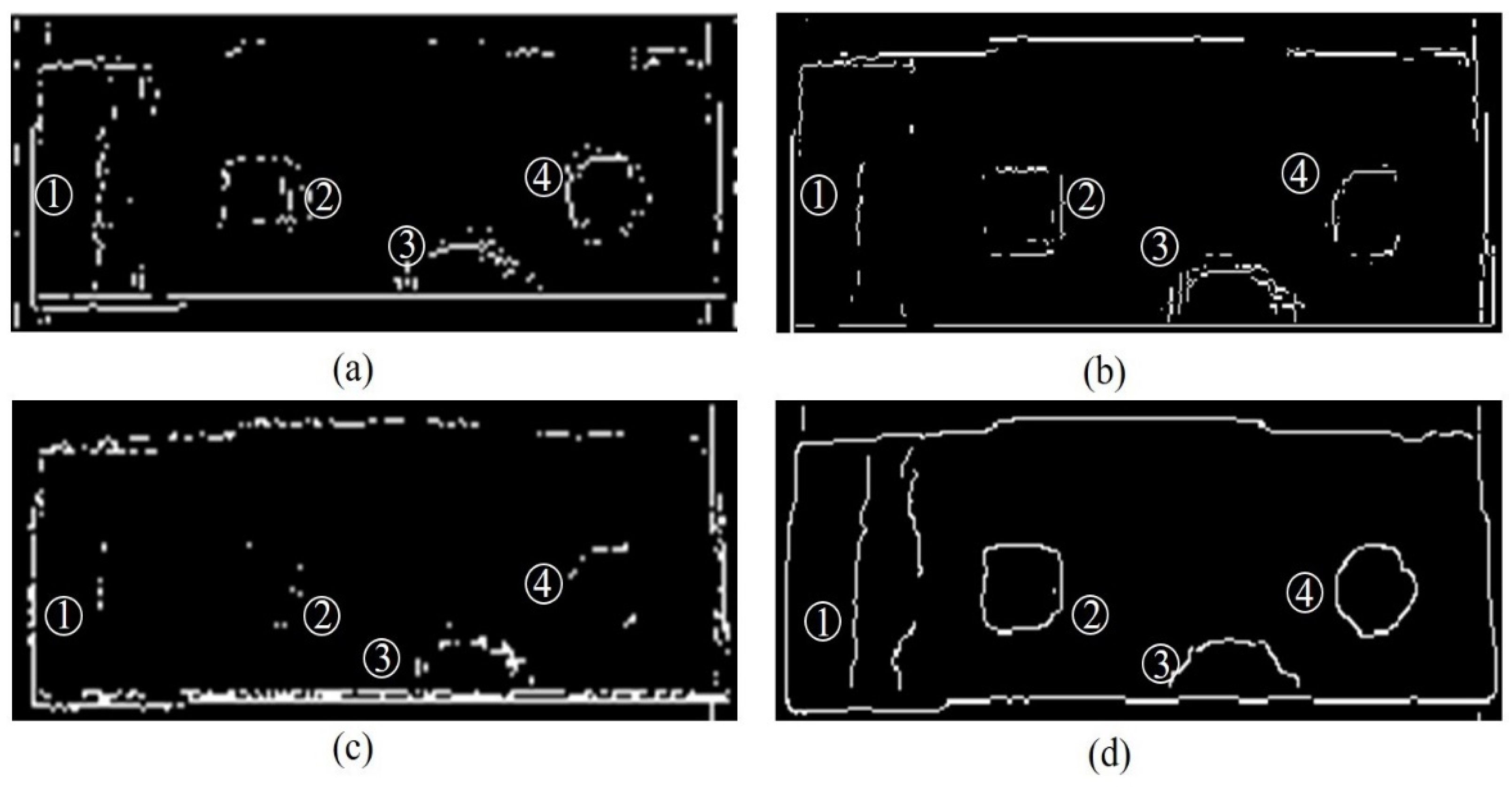
5.3. Canny Algorithm Analysis

The Canny operator [29,30] algorithm is used to extract the edge information from the filtered image. The resultant image using Sobel, Prewitt, and Roberts algorithms is also compared with the resultant image using Canny algorithm.

• Reprocessing the infrared image using a Gaussian filter;
• Calculation of gradient magnitude and direction;
• Nonmaximal value suppression;
• Dual thresholding algorithm to detect and connect edges;
• Edge connection.

Edge detection was performed on Figure 13 using the Canny operator. Figure 15 displays the images processed with different thresholds under the condition of σ = 1.5, while Figure 16 presents the results of dual-threshold detection at varying σ values. As shown in Figure 15 and Figure 16, adjusting parameters such as the Gaussian filter width, low threshold, and high threshold still fails to effectively resolve issues of edge loss and severe interference noise. Consequently, the defective contours of the HDPE film cannot be accurately identified.

Using the Canny operator for edge detection in Figure 14, the results of its processing are shown in Figure 17, from which it can be seen that the defect contour of No. 1 is almost completely lost after GIF-Canny and WGIF-Canny processing, while the defect contour is partially lost after WGIF-Canny and improves the GIF-Canny processing. No. 2 defect still has noise interference after GIF-Canny and WGIF-Canny processing, while the interference noise is significantly reduced after WGIF-Canny and improves the GIF-Canny. The edge contour of defect No.3 can be shown better after GIF-Canny and WGIF-Canny processing but there is noise interference, and the defect contour is completely lost after WGIF-Canny processing. After improving the GIF-Canny processing, the interference noise is obviously reduced, and the contour of the defect is relatively completely preserved. Defect No. 4 is processed by all four algorithms, the edge contour is well displayed, and there is almost no interference noise. Therefore, all four algorithms effectively preserve the edge information of defect No 4.

At the same time, the algorithms such as Sobel, Prewitt, and Roberts are compared with Canny’s algorithm [31,32]. As shown in Figure 18, after improving the GIF-Sobel, improving the GIF-Prewitt processing, all the defect edge contours are lost and there is noise interference, and, improving the GIF-Roberts processing, all the defect edge contours are lost seriously. The improvement in the GIF-Canny algorithm has a good retention of effective defect contours on the basis of noise reduction so that the final extracted defect contours are clear and effective.

In summary, the image processed by improving the GIF-Canny has a lower noise effect and retains effective defect edges, which can determine the contour of the defect and provide basic information for the next HDPE film defect remediation.

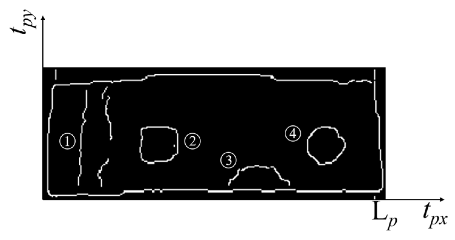
5.4. Calculation of Defect Length and Size Based on Edge Detection

With Figure 19 as the analysis object, according to the defect repair principles under actual working conditions, the direction of the weld seam is the same as the leakage repair direction. The proportional relationship is established between the total pixel value in the weld direction of the HDPE membrane and the actual physical value; the formula for calculating the weld defect size based on pixel analysis is as follows:

$$L_j={\displaystyle \frac{\mathrm{L}}{{\mathrm{L}}_p}}{d}_{p_j}$$

(15)

In Figure 19, $t_{px}$ and $t_{py}$ represent the pixel value size. In Equation (15), $\mathrm{L}$ is the weld length of the HDPE film, ${\mathrm{L}}_p$ is the total pixel value of the weld length of the HDPE film, $d_{p_j}$ is the total pixel value of weld defect, $L_j$ is the calculated defect size, and $j$ represents the defect numbers 1, 2, 3, and 4.

According to the four defects numbered 1, 2, 3, and 4 in Figure 19, we applied Formula (15) to calculate the defect lengths. The results are shown in

Table 4. Defect length dimension.

Defect Number	1	2	3	4
True size/cm	1.50	2.00	3.00	2.50
Calculate size/cm	1.56	2.20	3.19	2.33
Recognition error/%	4.6	10.0	6.3	6.8

.

6. Conclusions

In this paper, the distribution model of temperature difference characteristics is established, the defects of HDPE film surface defect are studied, and the temperature difference characteristics between the complete area and the defect area are analyzed; the shape of the defects in the weld area was also recognized and the size of the defects was determined by improving the test set-up.

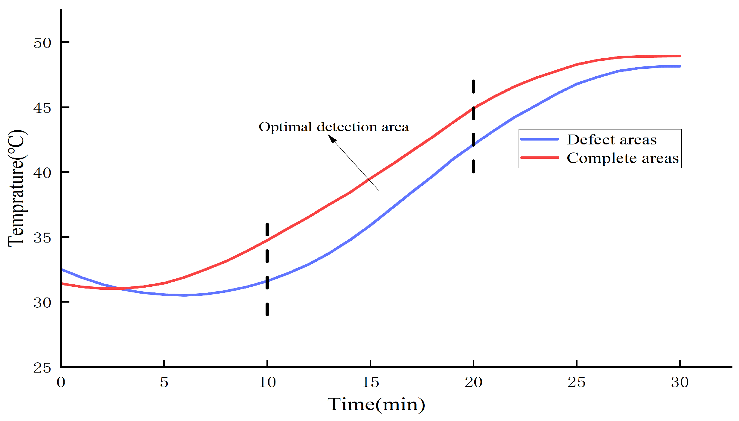
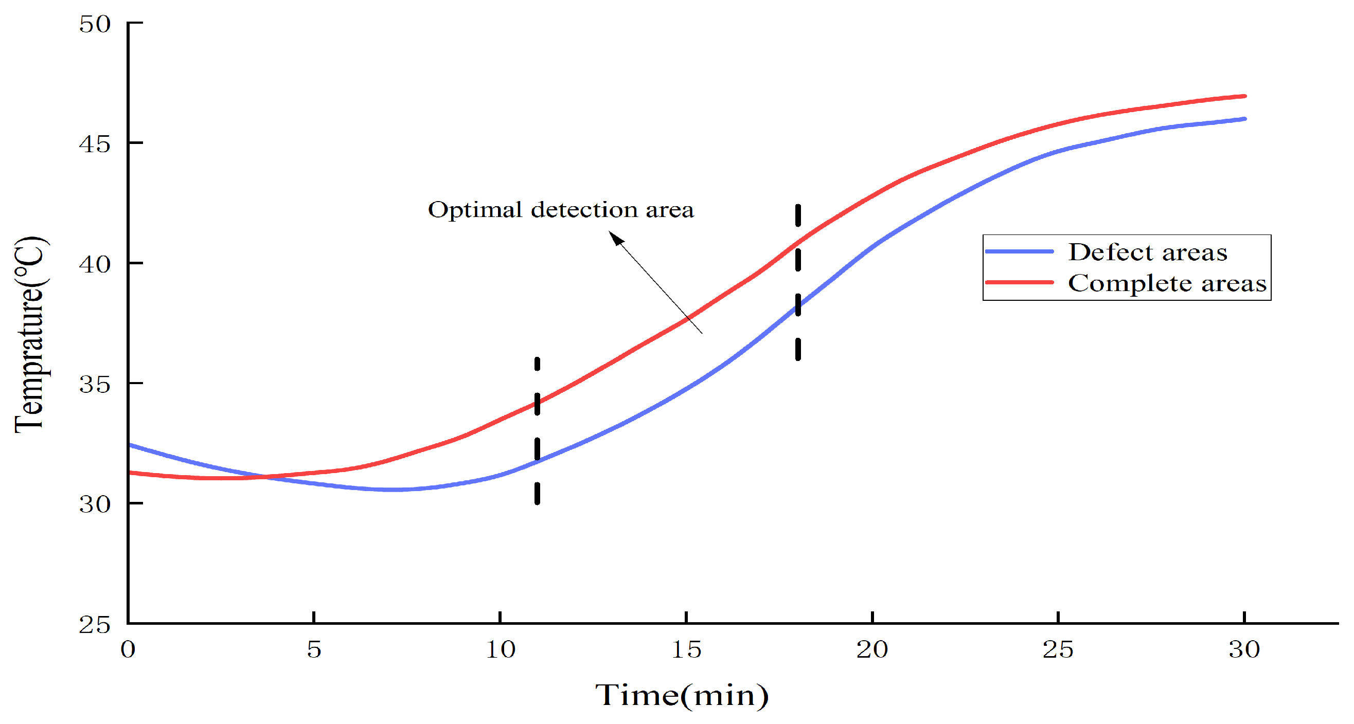
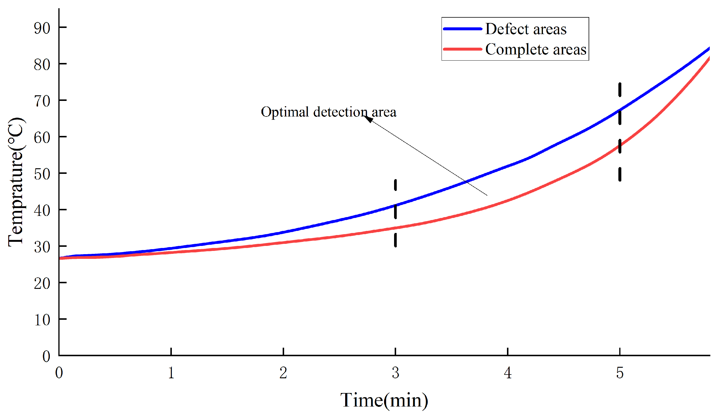
• Using temperature difference model can detect defects of the HDPE film in the state of bare film. Under the action of a continuous natural heat source, when the HDPE film is fully covered and tested, the continuous heating time is controlled at 10–20 min. The temperature difference between the defect area and complete area is obvious at the same time, which can be used as the best detection time domain for the whole film defect. For the detection of defects in the welding seam area, under the action of an active heating source, at 3–5 min, the temperature difference between defects in the welding seam area of the HDPE film and complete area is obvious. This period can be considered the optimal time for detecting defects in the weld area.
• Based on the research object of HDPE film infrared images, the recognition effect and characteristics of traditional classic edge detection algorithms are analyzed, and an HDPE defect edge detection algorithm combining improved guide image filtering and Canny is proposed. By performing denoising and edge retention on the collected image, the edge of the defect of the final image can be improved. Based on edge extraction, the defect size is estimated. The recognition error between defect size and actual size is not greater than 10%.
• Under the action of a heat source, HDPE film will have a temperature difference characteristic in the defect and complete area in the same time period. Based on this characteristic, the temperature difference model can detect HDPE film defect placement. It avoids contact damage to the film and realizes nondestructive testing of HDPE film.

For HDPE film defect detection, although this paper achieves the identification of defects on the surface of HDPE film and the contour recognition of defects in the weld area based on infrared detection technology, there are still inconvenient detection conditions in specific environments. So, in the follow-up research, the development of an infrared detection system of the piggybacking mechanism should be carried out to facilitate the detection system in order to adapt to the different environments and situations so as to make it more practical and effective.

References

1. Chen, Y.Y.; Sun, H.Y.; Zhang, W.; Huang, X.S. Using Stress Wave Technology for Leakage Detection in a Landfill Impervious Layer. Environ. Sci. Pollut. Res. 2019, 26, 32050–32064. [Google Scholar] [CrossRef] [PubMed]
2. Velenturf, A.P.M.; Purnell, P. Principles for a sustainable circular economy. Sustain. Prod. Consum. 2021, 27, 1437–1457. [Google Scholar] [CrossRef]
3. Pandey, L.M.S.; Shukla, S.K. An Insight into Waste Management in Australia with a Focus on Landfill Technology and Liner Leak Detection. J. Clean. Prod. 2019, 225, 1147–1154. [Google Scholar] [CrossRef]
4. Yuan, M.H.; Chiueh, P.T.; Lo, S.L. Understanding Synergies and Trade-Offs between Water and Energy Production at Landfill Sites. Sci. Total Environ. 2019, 687, 152–160. [Google Scholar] [CrossRef]
5. Sun, X.C.; Xu, Y.; Liu, Y.Q.; Nai, C.X.; Dong, L.; Liu, J.C.; Huang, Q.F. Evolution of Geomembrane Degradation and Defects in a Landfill: Impacts on Long-Term Leachate Leakage and Groundwater Quality. J. Clean. Prod. 2019, 224, 335–345. [Google Scholar] [CrossRef]
6. Spencer, M.W.; Cui, L.; Yoo, Y.; Paul, D.R. Morphology and Properties of Nanocomposites Based on HDPE/HDPE-g-MA Blends. Polymer 2010, 51, 1056–1070. [Google Scholar] [CrossRef]
7. Abdelaal, F.B.; Morsy, M.S.; Rowe, R.K. Long-term performance of a HDPE geomembrane stabilized with HALS in chlorinated water. Geotext. Geomembr. 2019, 47, 815–830. [Google Scholar] [CrossRef]
8. Abdelaal, F.B.; Rowe, R.K.; Islam, M.Z. Effect of leachate composition on the long-term performance of a HDPE geomembrane. Geotext. Geomembr. 2014, 42, 348–362. [Google Scholar] [CrossRef]
9. Zhuang, Y.; Seong, H.J.; Jang, Y.S. Environmental toxicity and decomposition of polyethylene. Ecotoxicol. Environ. Saf. 2022, 242, 113933. [Google Scholar] [CrossRef]
10. Huang, Y.X.; Meng, X.C.; Xie, Y.; Wan, L.; Lv, Z.L.; Cao, J.; Feng, J.C. Friction Stir Welding/Processing of Polymers and Polymer Matrix Composites. Compos. Part A Appl. Sci. Manuf. 2018, 105, 235–257. [Google Scholar] [CrossRef]
11. Peggs, I.D. Destructive Testing of Polyethylene Geomembrane Seams: Various Methods to Evaluate Seam Strength. Geotext. Geomembr. 1990, 9, 405–414. [Google Scholar] [CrossRef]
12. Casado, I.; Mahjoub, H.; Lovera, R.; Fernández, J.; Casas, A. Use of electrical tomography methods to determinate the extension and main migration routes of uncontrolled landfill leachates in fractured areas. Sci. Total Environ. 2015, 506–507, 546–553. [Google Scholar] [CrossRef] [PubMed]
13. Gilson-Beck, A. Controlling Leakage through Installed Geomembranes Using Electrical Leak Location. Geotext. Geomembr. 2019, 47, 697–710. [Google Scholar] [CrossRef]
14. Chen, Y.Y.; MA, T.H.; Chen, Y.; Bi, S.J.; Li, W.J.; Chen, X.Y.; Meng, C.R. Ultrasonic monitoring method of anti-seepage layer. Tech. Acoust. 2023, 4, 213–218. [Google Scholar] [CrossRef]
15. Avdelidis, N.P.; Moropoulou, A.; Marioli Riga, Z.P. The technology of composite patches and their structural reliability inspection using infrared imaging. Prog. Aerosp. Sci. 2003, 39, 317–328. [Google Scholar] [CrossRef]
16. Hassani, S.; Dackermann, U. A Systematic Review of Advanced Sensor Technologies for Non-Destructive Testing and Structural Health Monitoring. Sensors 2023, 23, 2204. [Google Scholar] [CrossRef]
17. Qu, Z.; Jiang, P.; Zhang, W. Development and Application of Infrared Thermography Non-Destructive Testing Techniques. Sensors 2020, 20, 3851. [Google Scholar] [CrossRef]
18. Ma, Y.; Rose, F.; Wong, L.; Vien, B.S.; Kuen, T.; Rajic, N.; Kodikara, J.; Chiu, W. Detection of Defects in Geomembranes Using Quasi-Active Infrared Thermography. Sensors 2021, 21, 5365. [Google Scholar] [CrossRef]
19. Liu, J.Y.; Tang, Q.J.; Wang, Y.; Lu, Y.M.; Zhang, Z.P. Defects’ Geometric Feature Recognition Based on Infrared Image Edge Detection. Infrared Phys. Technol. 2014, 67, 387–390. [Google Scholar] [CrossRef]
20. Zeng, J.L.; Chang, B.H.; Du, D.; Hong, Y.X.; Zou, Y.R.; Chang, S.H. A Visual Weld Edge Recognition Method Based on Light and Shadow Feature Construction Using Directional Lighting. J. Manuf. Process. 2016, 24, 19–30. [Google Scholar] [CrossRef]
21. Dong, S.H.; Sun, X.; Xie, S.Y.; Wang, M.F. Automatic Defect Identification Technology of Digital Image of Pipeline Weld. Nat. Gas Ind. B 2019, 4, 399–403. [Google Scholar] [CrossRef]
22. Han, J.; Yue, J.; Zhang, Y.; Bai, L.F. Salient Contour Extraction from Complex Natural Scene in Night Vision Image. Infrared Phys. Technol. 2014, 63, 165–177. [Google Scholar] [CrossRef]
23. Hsu, C.Y.; Wang, H.F.; Wang, H.C.; Tseng, K.K. Automatic Extraction of Face Contours in Images and Videos. Future Gener. Comput. Syst. 2012, 28, 322–335. [Google Scholar] [CrossRef]
24. Rong, S.H.; Zhou, H.X.; Qin, H.L.; Lai, R.; Qian, K. Guided Filter and Adaptive Learning Rate Based Non-Uniformity Correction Algorithm for Infrared Focal Plane Array. Infrared Phys. Technol. 2016, 76, 691–697. [Google Scholar] [CrossRef]
25. Liu, N.; Zhang, Y.Y.; Xie, J.; Yu, J.H.; Xiao, H.Y.; Min, T.Y. A Novel High Dynamic Range Image Enhancement Algorithm Based on Guided Image Filter. Optik 2015, 126, 4581–4585. [Google Scholar] [CrossRef]
26. Geethu, H.; Shamna, S.; Kizhakkethottam, J.J. Weighted Guided Image Filtering and Haze Removal in Single Image. Procedia Technol. 2016, 24, 1475–1482. [Google Scholar] [CrossRef]
27. Li, Z.G.; Zheng, J.H.; Zhu, Z.J.; Yao, W.; Wu, S.Q. Weighted Guided Image Filtering. IEEE Trans. Image Process. 2015, 24, 120–129. [Google Scholar] [CrossRef]
28. Chen, B.; Wu, S.Q. Weighted aggregation for guided image filtering. Signal Image Video Process. 2019, 14, 491–498. [Google Scholar] [CrossRef]
29. Biswas, R.; Sil, J. An Improved Canny Edge Detection Algorithm Based on Type-2 Fuzzy Sets. Procedia Technol. 2012, 4, 820–824. [Google Scholar] [CrossRef]
30. Zhang, X.F.; Zhang, Y.; Zheng, R. Image Edge Detection Method of Combining Wavelet Lift with Canny Operator. Procedia Eng. 2011, 15, 1335–1339. [Google Scholar] [CrossRef]
31. Liu, C.; Shirowzhan, S.; Sepasgozar, S.M.E.; Kaboli, A. Evaluation of Classical Operators and Fuzzy Logic Algorithms for Edge Detection of Panels at Exterior Cladding of Buildings. Buildings 2019, 9, 40. [Google Scholar] [CrossRef]
32. Zhang, A.A.; Li, Q.J.; Wang, K.C.P.; Shi, Q. Matched Filtering Algorithm for Pavement Cracking Detection. Transp. Res. Rec. 2013, 2367, 30–42. [Google Scholar] [CrossRef]
Figure 1. Infrared imaging detection of HDPE film defects.
Applsci 15 04774 g001
Figure 2. Schematic diagram of heat conduction in the defect area.
Applsci 15 04774 g002
Figure 3. Schematic diagram of infrared temperature difference image acquisition for different defects.
Applsci 15 04774 g003
Figure 4. Damage diagram of HDPE film.
Applsci 15 04774 g004
Figure 5. Infrared timing diagram for 0.15 cm HDPE film: (a) t = 0.0 min; (b) t = 0.5 min; (c) t = 10.0 min; (d) t = 11.0 min; (e) t = 12.0 min; (f) t = 13.0 min; (g) t = 20.0 min; (h) t = 21.0 min; (i) t = 25.0 min.
Applsci 15 04774 g005
Figure 6. Infrared timing diagram for 0.20 cm HDPE film: (a) t = 0.0 min; (b) t = 0.5 min; (c) t = 10.0 min; (d) t = 11.0 min; (e) t = 12.0 min; (f) t = 13.0 min; (g) t = 20.0 min; (h) t = 21.0 min; (i) t = 25.0 min.
Applsci 15 04774 g006
Figure 7. HDPE film of 0.15 cm defective–complete area temperature change curve.
Applsci 15 04774 g007
Figure 8. HDPE film of 0.20 cm defective–complete area temperature change curve.
Applsci 15 04774 g008
Figure 9. HDPE film weld defect detection infrared thermal imaging system diagram.
Applsci 15 04774 g009
Figure 10. Schematic diagram of weld defects.
Applsci 15 04774 g010
Figure 11. Infrared timing diagram of HDPE film weld defect detection: (a) t = 0.0 min; (b) t = 1.0 min; (c) t = 2.0 min; (d) t = 3.0 min; (e) t = 4.0 min; (f) t = 5.0 min.
Applsci 15 04774 g011
Figure 12. Weld defective–complete area temperature change curve.
Applsci 15 04774 g012
Figure 13. Inputting the original image.
Applsci 15 04774 g013
Figure 14. Comparison of different bootstrap filtering algorithms: (a) GIF; (b) WGIF; (c) WAGIF; (d) improve the GIF.
Applsci 15 04774 g014
Figure 15. Canny edge detection of input original image at σ = 1.5: (a) low threshold processing; (b) bilateral threshold processing; (c) high threshold processing.
Applsci 15 04774 g015
Figure 16. Canny bilateral threshold edge detection for input original image: (a) σ = 1; (b) σ = 1.5; (c) σ = 3.
Applsci 15 04774 g016
Figure 17. Comparison of defective edge extraction effects of Canny algorithm: (a) GIF-Canny; (b) WGIF-Canny; (c) WAGIF-Canny; (d) improve the GIF-Canny.
Applsci 15 04774 g017
Figure 18. Comparison of the effect of different edge extraction algorithms: (a) improve the GIF- Sobel; (b) improve the GIF-Prewitt; (c) improve the GIF-Roberts; (d) improve the GIF-Canny.
Applsci 15 04774 g018
Figure 19. Pixel analysis of defect size.
Applsci 15 04774 g019