Article

A Novel Temperature Reconstruction Method for Acoustic Pyrometry Under Strong Temperature Gradients and Limited Measurement Points

by
Jingkao Tan
1,
Lehang Chen
1,
Na Li
1,*,
Qulan Zhou
1,
Zhongquan Gao
1 and
Jie Zhou
2
1
State Key Laboratory of Multiphase Flow in Power Engineering, Xi’an Jiaotong University, Xi’an 710049, China
2
Xi’an Aerospace Propulsion Institution, Xi’an 710100, China
*
Author to whom correspondence should be addressed.
Appl. Sci. 2025, 15(9), 4728; https://doi.org/10.3390/app15094728
Submission received: 28 February 2025 / Revised: 21 April 2025 / Accepted: 23 April 2025 / Published: 24 April 2025

Abstract

:
Acoustic pyrometry (AP) is a promising methodology for high-quality temperature field reconstruction, which is widely used in the monitoring of atmosphere, room, and furnace. However, most of the existing acoustic reconstruction algorithms are developed and utilized in relatively uniform temperature distributions. Furthermore, their ability of tracking hotspots are rarely discussed. This paper first proposed the coefficient of heating effect (CHE) to quantitatively assess the intrinsic characteristics of the reconstructed temperature field. Aiming to accurately reconstruct the temperature fields under strong gradients and limited measurement points, this paper presents a novel temperature reconstruction method based on the adaptive hybrid kernel (AHK) and the adaptive grid evolution strategy (AGES). The proposed AGES-AHK method implements adaptive hybrid kernel adjustments on AGES-optimized nonuniform grids, achieving significant improvements in both reconstruction fidelity and hotspot characterization. The reconstruction results show that at CHE levels below 15, the AGES-AHK method achieved the normalized root mean square error (NRMSE) of less than 3.7%, the hotspot position deviation Dh of less than 2.3% and the hotspot temperature error Eh of less than 15%, improving reconstruction accuracy by more than 33% compared to the basis method. Qualitative and quantitative analyses demonstrate the AGES-AHK method’s superior performance in challenging conditions.

1. Introduction

The temperature distribution in a furnace has a direct effect on fuel combustion efficiency and equipment safety during the operation of industrial combustion devices, reflecting the emission evolution and combustion process [1,2]. The analysis of the temperature field in furnaces helps to improve combustion efficiency, reduce pollutant emissions, and prevent security incidents [3,4,5].
Acoustic pyrometry (AP) is a noninvasive temperature measurement technique. The region of interest (ROI) is first discretized by meshing, and the temperature and sound velocity within each grid are treated as unity values. Acoustic transceivers are then placed at the edge of the ROI, and the time of flight (TOF) of multiple acoustic propagation paths in the ROI is measured. Based on the dependencies of sound velocity and temperature, the grid-averaged temperature is solved by a reconstruction algorithm. AP has a wide measurement range, quick dynamic response and good environmental adaptability. In addition, acoustic transducers are smaller and easier to install than other noncontact sensors. Therefore, AP is widely used to obtain the temperature distribution in boiler furnaces [1,3,6,7] and gases [8,9,10].
Currently, researchers are focusing their investigations on improving the reconstruction algorithms for acoustic pyrometry, including the iterative method [1,11,12,13], the truncated singular value decomposition (TSVD) [14,15,16,17], and the least square method (LSM) [18,19,20,21]. Many researchers have devoted their efforts to improving the reconstruction performance of AP based on different reconstruction algorithms, yielding remarkable outcomes. The main objective of a reconstruction algorithm is to mitigate the difference between the theoretical data and actual data and to use this information to correct the value of the average temperature value inside each grid.
These outcomes have been applied for industrial temperature monitoring. Bramanti [3] proposed and applied two classes of acoustic reconstruction algorithms to both simulated and experimental data measured in power plants of the Italian National Electricity Board. Yan [22] proposed a temperature monitoring method based on acoustic pyrometry for the early prediction of temperature anomalies in stored grain. By improving the iterative method and the time delay estimation method, Zhang [1] used acoustic computed tomography technology to obtain the temperature profile of a furnace cross-section in a domestic 600-MW coal-fired boiler.
In addition to temperature measurements, the achievements in the field of acoustic pyrometry are also used in other related industrial applications. Zhang [7,23] adopted acoustic pyrometry to monitor the changes of the flue gas temperature near the heat surface and thus proposed a new clean factor to monitor the ash fouling in a domestic 330-MW unit manufactured by the Babcock & Wilcox Company. Kong [24] applied acoustic tomography combined with radial basis function artificial neural network for coordinate estimation to locate the leakage from a water-cooling wall tube.
However, most of the existing acoustic temperature distribution reconstruction algorithms are developed and modified with relatively uniform temperature distribution environments [11,25,26,27]. Unfortunately, under strong temperature gradients, these reconstruction algorithms are almost incapable of performing accurate measurements [28,29]. This phenomenon can be attributed to two primary factors. First, the domain discretization assumption eliminates the details of continuously varying temperatures within the ROI, only resulting in limited grid-averaged values. Furthermore, the domain discretization causes remarkable discretization errors in high gradient regions. Second, the sparse data from limited transducer placements results in an ill-posed AP problem, exacerbating the difficulty of reconstructing temperature fields with high gradient variations and increasing the grid reconstruction errors. The superposition of grid reconstruction errors with discretization errors results in the difficulty of reproducing temperature distributions under strong temperature gradients within a reliably reconstructed grid size.
Consequently, some researchers have enhanced the reconstruction process beyond the reconstruction algorithm, thereby improving AP reconstruction performance. For the modification of domain discretization, Barathula [30] used appropriate central nonuniform domain discretization and transceiver collocation to significantly improve the accuracy of acoustic pyrometry. Pal [25] successfully tracked the shift pattern of the hotspot via the spatial moving sample (SMS) method on hexagonal meshing. Based on the coarse grid temperature averages obtained from the reconstruction algorithm, Liu [11] and Zhang [31] built neural networks to predict the temperature distribution on a refined grid. However, the nonuniform discretization proposed by Barathula is fixed at the center and requires a large number of transceivers (at least 44). The objective of Pal’s study is a simple temperature field with single heat source in a small circular region. And it is difficult to obtain sufficient reliable sample data, which limits the practicability of neural networks.
In this research, a novel temperature reconstruction method for acoustic pyrometry under strong temperature gradients and limited measurement points is proposed and demonstrated. The key metrics include the reconstruction accuracy, the accuracy of peak temperatures and hotspot positions. To quantitatively assess the temperature gradient of the reconstructed temperature field, the coefficient of heating effect (CHE) is first proposed, and the existing acoustic temperature tomography studies are evaluated [4,6,11,14,17,20,28,32,33,34,35,36,37,38,39]. Then, an adaptive hybrid kernel method based on Multiquadric (MQ) and Gaussian (G) radial basis function was proposed and utilized to reconstruct the temperature field. After that, the effect of nonuniform meshes on improving performance is investigated and a novel adaptive grid evolution strategy (AGES) is introduced. Consequently, the finalized AGES-AHK method implements adaptive kernel adjustments on AGES-optimized nonuniform grids, integrating the optimization of AHK and AGES. The primary benefit of the proposed AGES-AHK method lies in its ability to accurately reconstruct temperature fields under strong gradients and limited measurement points, whereas traditional acoustic pyrometry methods typically fail. In comparison to conventional approaches which rely on the uniform grid discretization and a fixed radial basis function approximation, the AGES-AHK method adaptively optimizes both the grid density and the kernel functions based on the specific characteristics of the temperature field, which allows for precise tracking of hotspots and significantly improved reconstruction accuracy. Qualitative and quantitative analyses demonstrate the AGES-AHK method’s superior performance in challenging conditions.

2. Basic Principles and Methodologies

2.1. Basic Principle of Acoustic Pyrometry

Acoustic pyrometry (AP) is a noninvasive temperature measurement technique. The region of interest (ROI) is first discretized by meshing, and the temperature and sound velocity within each grid are treated as unity values. Acoustic transceivers are then placed at the edge of the ROI, and the time of flight (TOF) of multiple acoustic propagation paths in the ROI is measured. Based on the dependencies of sound velocity and temperature, the grid-averaged temperature is solved by a reconstruction algorithm.
Theoretically, the sound velocity depends on the gas temperature [3]:
c = γ R M T = Z T
where c is the sonic velocity (m/s), γ is the adiabatic gas constant, R is the molar gas constant with a value of 8.314 J/(mol∙K), M is the average molecular weight of gas (g/mol), T is the absolute temperature (K), and Z is a coefficient determined by γ, M and R. The acoustic time of flight (TOF) can be obtained via integration along the acoustic path l [3]:
t = 1 c d l = f d l
where f is the reciprocal of sound velocity at specific ROI point (s/m), which is termed “slowness”, and t is the TOF.
The average temperature of the acoustic path can be obtained by calculating the reciprocal of sound velocity via the TOF. Similarly, the average temperature of the grid can be obtained by solving the linear equations subsequent to the grid division.
l 11 l 12 l 1 N l 21 l 22 l 2 N l M 1 l M 2 l M N f 1 f 2 f N = t 1 t 2 t M A x = b
where lij is the length of the i-th acoustic path through the j-th grid; fj is the reciprocal of sound velocity in the j-th grid of the ROI; ti is the TOF of the i-th acoustic path; M and N are the number of acoustic paths and the number of ROI grids, respectively; A is the coefficient matrix; b is the TOF matrix; and the unknown x is the reciprocal of sound velocity matrix.
Based on the dependence of the acoustic velocity on temperature, the temperature distribution can be reconstructed by measuring the TOF between pairs of acoustic transducers in the ROI. In fact, the number of grids that each acoustic path passes through is less than N. Therefore, the coefficient matrix A in Equation (3) contains many null-space components, resulting in the ill-conditioned nature of the problem, which is difficult to solve accurately via general methods [40].
When acoustic waves propagate through a nonuniform temperature field, they bend because of the change in propagation velocity [21]. In early studies, researchers simplified the acoustic paths into a linear model of the connection between acoustic transducers, resulting in a deviation from the true value and a maximum reconstruction error of 20% based on the linear propagation model [41,42].
According to Fermat’s principle, the differential equation satisfied by acoustic wave propagation in a two-dimensional temperature field can be derived from the Euler formula [21,34]:
y = 1 + y 2 2 T ( x , y ) y T ( x , y ) x T ( x , y ) y , y SA = y ( x ) | x = x SA y EB = y ( x ) | x = x EB
where (x, y) represents the 2D coordinates of discrete points; y′ and y″ represent the first-order and second-order derivatives of y, respectively; SA and EB are the two acoustic transducers. The target acoustic path curve we need is the acoustic path starting at the transceiver SA and ending at EB.
Therefore, it can be seen from Equation (4) that the solution of two-dimensional planar acoustic curve is a typical second-order ordinary differential boundary value problem, which can be solved by shooting methods [43].

2.2. The Coefficient of Heating Effect

The domain discretization assumption, combined with the limited number of acoustic transceivers, results in sparse valid data and an ill-posed AP problem. Moreover, as the complexity or temperature gradient of the temperature phantom rises, the ill-conditioned nature of the reconstruction problem becomes more severe. Since most of the existing acoustic temperature distribution reconstruction algorithms are developed and modified with relatively uniform temperature distribution environments [11,25,26,27], a quantitative evaluation criterion is needed to assess the reconstruction difficulty of the temperature phantoms.
Consequently, considering the gradient and complexity of the temperature phantom, a dimensionless parameter CHE was proposed to assess the reconstruction difficulty as follows:
T mid = ( T max T min ) / 2 , P TD = T max T min T max + T min S HT S ROI , C HE = n HS P TD
where Tmax and Tmin are the maximum and minimum temperatures within the ROI, respectively. Tmid is the middle temperature of the temperature phantom, and regions above this temperature are considered to be high-temperature regions; SHT and SROI represent the area of the high-temperature regions and the overall area of the ROI, respectively. PTD (Proportion of Temperature Difference) is a dimensionless proportion of the temperature change within the heating zone, representing the relative temperature gradient within the ROI and the extent of the high temperature regions. nHS is the number of heat sources within the ROI, representing the complexity of the temperature phantom. Thus CHE (Coefficient of heating effect) is a dimensionless parameter that simultaneously takes into account the number of heat sources, the temperature gradient and the heating range, -representing the comprehensive complexity as well as the reconstructing difficulty of the temperature phantom within the ROI range.
It is well-established that the reconstruction accuracy of acoustic tomography is influenced by multiple factors [16], including reconstruction algorithms, parameter selection, domain discretization, and the intrinsic characteristics of the reconstructed temperature field (CHE). To exclusively investigate the influence of CHE on reconstruction performance, a systematic review of 15 articles [4,6,11,14,17,20,28,32,33,34,35,36,37,38,39] published since 2015, denoted in citation order as Ref 1 to Ref 15, was conducted. In these studies, after finalizing grid configurations, researchers applied proprietary enhancement methodologies to reconstruct multiple temperature phantoms. Based on the phantom designs and region-of-interest (ROI) selections reported in these studies, the CHE values for all temperature fields were calculated. Subsequently, the root mean square error (RMSE) of the reconstruction results in each study was correlated with its corresponding CHE value, as illustrated in Figure 1.
As shown in Figure 1, the RMSE exhibits a significant positive correlation with the CHE of the temperature phantom in all 15 papers [4,6,11,14,17,20,28,32,33,34,35,36,37,38,39], indicating that the intrinsic characteristics of the reconstructed temperature field (CHE) have a direct effect on reconstruction fidelity.
Furthermore, the temperature phantoms used in all 15 papers exhibit CHE values below 5 and demonstrate adequate reconstruction accuracy, with RMSE values below 8.5%. It should be noted that the temperature phantoms in Ref 11 to Ref 14 [35,36,37,38] are reproduced from measured hot-state temperature data provided by a real boiler plant, and their CHE values are less than 1.2, which belong to the relatively uniform temperature distributions and are suitable for most of the existing reconstruction algorithms.

2.3. Improvements to the Reconstruction of High-Gradient Temperature Fields with Limited Measurement Points

In high-gradient temperature fields with limited measurement points, the reconstruction of the AP is an ill-posed problem with sparse valid data. Therefore, two improvements to the reconstruction process have been primarily proposed. First, the hybrid kernel method can improve the reconstruction accuracy to a limited extent by adjusting the ratio of different basis functions in the hybrid kernel, thereby ensuring a more accurate RBF approximation and improving the overall reconstruction accuracy. Second, inspired by the CFD simulation in which refined meshes are employed for modelling complex parts to achieve enhanced results, local mesh refinement for hotspot regions is considered to simultaneously improve both overall reconstruction accuracy and hotspot tracking performance.

2.3.1. RBF Approximation and the Adaptive Hybrid Kernel Method

The solvability of linear equations requires that the number of grids must not exceed the number of acoustic propagation paths [40] when the general domain discretization assumption is used to solve reconstruction problems, thus restricting the reconstruction performance of the algorithm. The RBF-based reconstruction algorithms do not have this strict constraint [34,44], allowing the number of ROI grids to be selected according to actual needs through RBF approximation.
The ROI is divided into N grids. Directly determining the distribution of the reciprocal of sound velocity f is difficult due to the complexity of its functional expression. However, f can be expanded into a linear combination of kernel functions through RBF interpolation [44,45]:
f ( x , y ) = i = 1 N λ i ϕ i
where λi represents the respective coefficient when the nonlinear function forms a linear combination ϕi represents a nonlinear function with an independent variable of Euclidean distance r. The expression of ϕ(r) in two dimensions [45] is as follows:
ϕ ( r ) = ϕ ( x , y ) = ϕ ( x i x ) 2 + ( y i y ) 2
where (xi, yi) represents the coordinates of the known points, which are the centers of the N grids, (x, y) represents the coordinates of the target point to be expanded, and r is the Euclidean distance between the known point and the target point.
In the context of acoustic pyrometry, the RBF approximation is equivalent to the process of interpolating the unknown acoustic velocity field prior to reconstruction. However, this preliminary interpolation may not entirely align with the inherent field characteristics, resulting in deviations of the reconstructed values from the true values. Consequently, the type and shape parameter of the RBF are critical for the accuracy of the reconstruction [16]. The commonly used Gaussian (G) and Multiquadric (MQ) radial basis functions were selected for acoustic reconstruction [45,46]:
G a u s s i a n : M u l t i q u a d r i c : ϕ G ( r ) = exp ( ε 2 r 2 ) ϕ M Q ( r ) = 1 + ε 2 r 2
where ε is the shape parameter. For uniformity and convenience, ε is defined as the coefficient of the Euclidean distance r, as shown in Equation (8).
The coefficient of linear combination can be calculated according to the known points:
ϕ 1 ( x 1 , y 1 ) ϕ 2 ( x 1 , y 1 ) ϕ N ( x 1 , y 1 ) ϕ 1 ( x 2 , y 2 ) ϕ 2 ( x 2 , y 2 ) ϕ N ( x 2 , y 2 ) ϕ 1 ( x N , y N ) ϕ 2 ( x N , y N ) ϕ N ( x N , y N ) λ 1 λ 2 λ N = f 1 f 2 f N ϕ λ = x
Substitution of Equation (9) back into Equation (3) yields the following result:
A x = b A ϕ λ = b B λ = b
The problem of finding x in Equation (3) is transformed to finding λ in Equation (10). The matrix B containing RBF information replaces the original coefficient matrix A, recovering the null-space component and reducing the ill-conditioned nature of the problem. Specifically, λ in Equation (10) is solved by the reconstruction algorithm; then, the reciprocal of sound velocity matrix x is obtained from Equation (9), and the average temperatures of the ROI grids are reconstructed through Equation (1).
Unfortunately, under the strong temperature gradients, the existing RBF-based reconstruction algorithms encounter significant challenges in achieving precise measurement outcomes. Luckily, the integration of hybrid kernel methods has been demonstrated to enhance the overall reconstruction performance to a limited extent by adjusting the ratio of different basis functions in the hybrid kernel [28,29].
The fundamental principle of the hybrid kernel method resides in the integration of multiple kernel functions, thereby synthesizing their complementary advantages to establish a versatile framework for addressing complex data challenges. For example, Mishra [29] applied a combination of the Gaussian and cubic (Φ(r) = r3) functions. Yu [29] proposed a hybrid function using a combination of the cubic kernel and the exponential correlation function (Φ(r) = eεr). In interpolation scenarios where datasets concurrently exhibit localized nonlinearities and global trends, hybrid kernels demonstrate superior capability in balancing these competing fitting requirements.
It is observed that both the cubic kernel and the exponential correlation function have their own disadvantages for accomplishing the reconstruction task. While the cubic function is finitely smooth and unhampered by shape parameter, using the cubic kernel may lead to the singular problem at some scattered locations. The exponential kernel does not fully balance the distances and randomness among the data points. Consequently, an improved hybrid kernel using a different basis function combination was proposed.
As the most commonly used RBF, G-RBF has sharp spatial localization characteristics that enhance its suitability for reconstructing complex temperature fields in the furnace with less measured data [36,38]. MQ-RBF is a reliable method for thermal image distribution reconstruction [26]. As shown in Equation (8), the value range of MQ-RBF is significantly broader than that of G-RBF. Furthermore, MQ-RBF is not sensitive to the change of shape parameters [36,38], which leads to a wide optimal range of shape parameters and good global characterization.
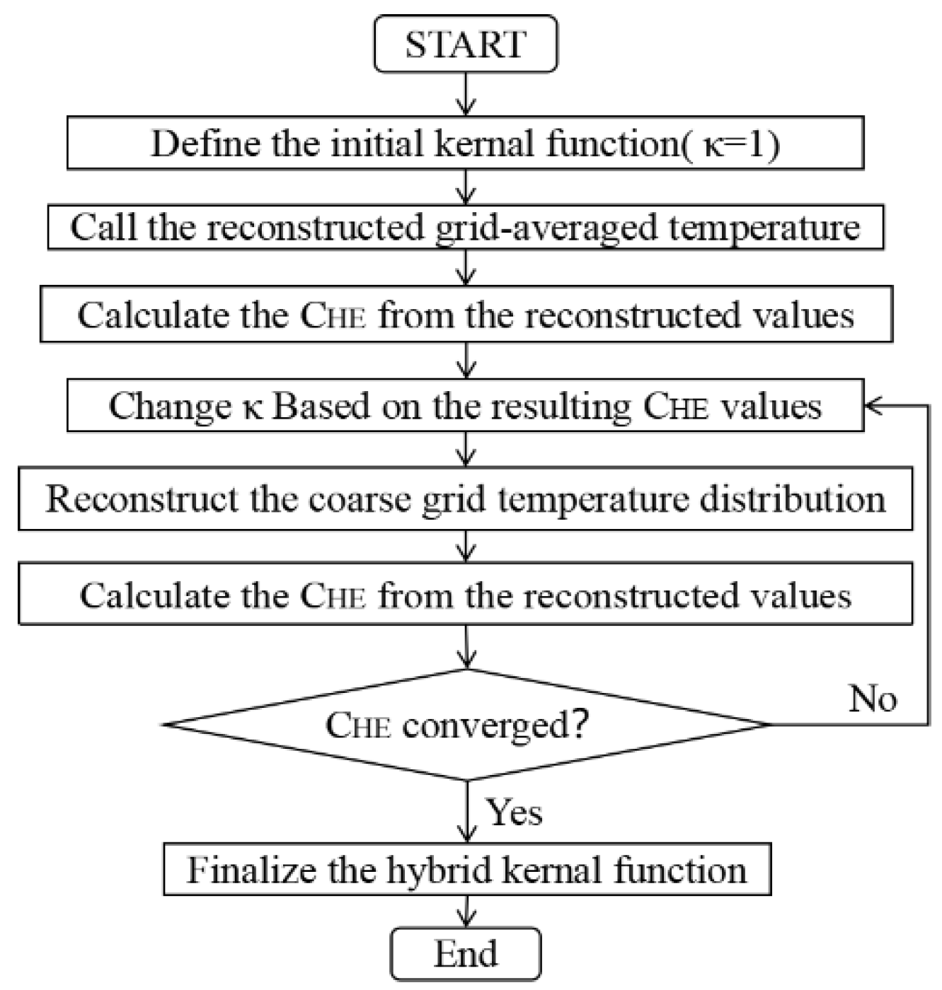
Therefore, an adaptive hybrid kernel method (AHK) based on MQ and G radial basis functions was proposed, as shown in Equation (11) and Figure 2. The purpose of this method is to dynamically adjust kernel weights based on the data, with a view to further enhancing generalization capabilities.
ϕ A H K ( r ) = κ 1 + ε 1 2 r 2 + exp ( ε 2 2 r 2 )
where ε1 and ε2 are the shape parameters associated with the RBFs, which can be determined through parametric investigation. And κ is a weight coefficient that controls the contribution of the G and MQ kernel function in the improved hybrid kernel. This combination has the advantage that the involvement of the Gaussian kernel in the improved hybrid method helps to regulate when the weight coefficient κ is very small.
The flow chart of the AHK method is shown in Figure 2. Due to the relationship between the value range of MQ and G, the κ in Equation (11) is initially set to 1 and the temperature field is first reconstructed mainly by the global properties of MQ. The grid-scale CHE is calculated and the complexity of the reconstructed temperature field is initially assessed. Subsequently, the proportion of G in the hybrid kernel is augmented by decreasing the κ value to accommodate the localized nonlinearities of the temperature phantom. It is imperative to repeatedly adjust the κ value until the calculated CHE value converges, thus enabling the determination of the finalized adaptive hybrid kernel. The finalized adaptive hybrid kernel from the AHK method combines the sharp spatial localization characteristics of G with the global characterization of MQ.

2.3.2. Domain Discretization and the Adaptive Grid Evolution Strategy

Due to the limited number of acoustic sensors and the sparse valid data of the ill-posed AP problem, the domain discretization assumption was adopted in most of the existing reconstruction method. That is, the ROI is divided into N small grids/cells, and the gas parameter (temperature, sound velocity, etc.) within each cell is considered as a uniform value. Then based on the dependencies of sound velocity and temperature, the grid-averaged temperature is solved by a reconstruction algorithm.
Theoretically, the length of the sound path traveling through each cell determines its temperature. Tracking the distribution of each path length in the whole domain is crucial. The discretization of the domain affects the accuracy of acoustic pyrometry. Although uniform discretization and square grids are widely used because of their simplicity and reliability, they also restrict the potential for further optimization of domain discretization [47]. Barathula [30] used appropriate central nonuniform domain discretization and transceiver collocation to significantly improve the accuracy of acoustic pyrometry. Pal [25] successfully tracked the shift pattern of the hotspot via the spatial moving sample (SMS) method. Specifically, the distribution of uniform hexagonal grids was iteratively shifted to increase the number of acoustic paths in the hotspot grid. Therefore, the SMS method and nonuniform discretization were combined to develop the adaptive grid evolution strategy (AGES) in this paper.
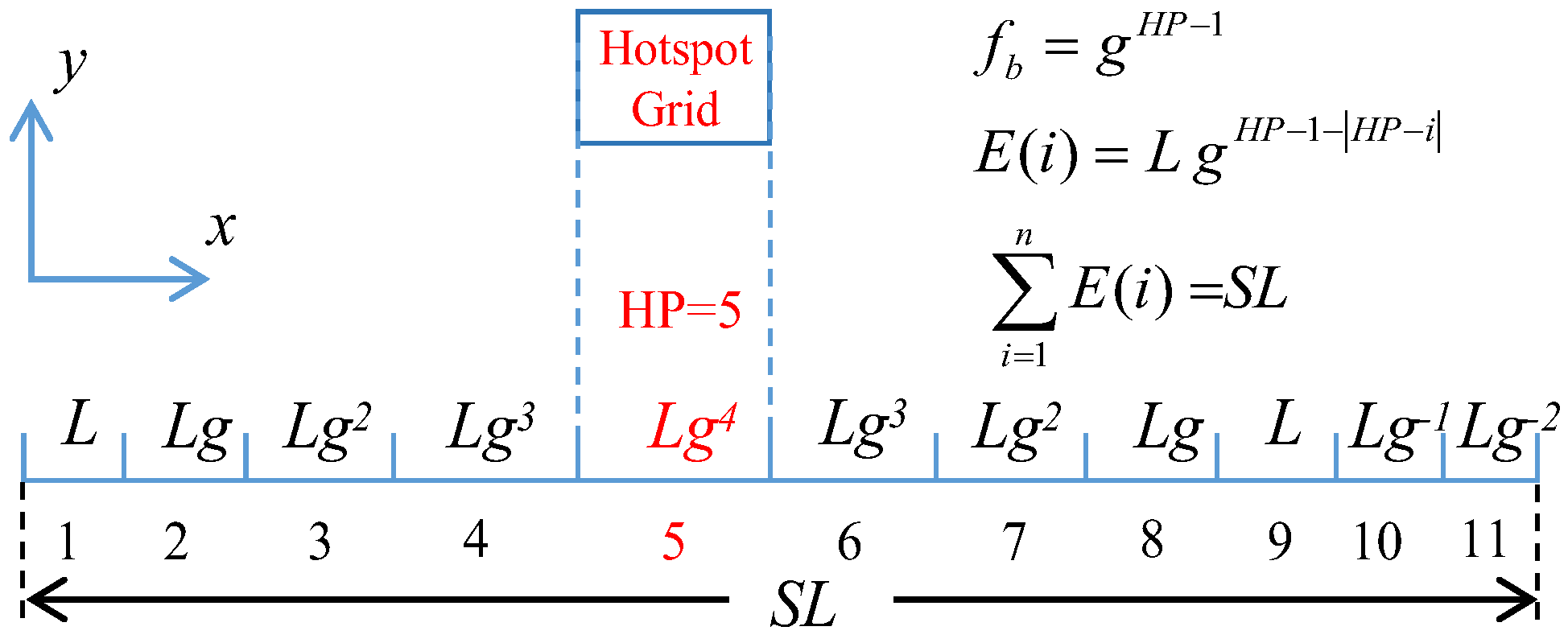
Different cell sizes ranging from finer grids to coarser grids are considered, while keeping the number of grids constant. The cell sizes are determined via nonuniform discretization as shown in Figure 3. A hotspot is defined as the local highest temperature point [25,46]. With n = 11, the hotspot grid is located in the HPth division in the x direction. fb is the bias factor, which represents the degree of inhomogeneity across the mesh, and g is the growth rate. When fb = 1, the AGES undergoes uniform discretization. E(i) is the length of the ith division in the x direction, L is the length of the first element, and SL is the side length of the ROI; that is, the side length of the hotspot grid is fb times that of the first grid. The lengths of the divisions away from the hotspot grid are in a geometric series. The domain discretization in the y direction is identical to that in the x direction.
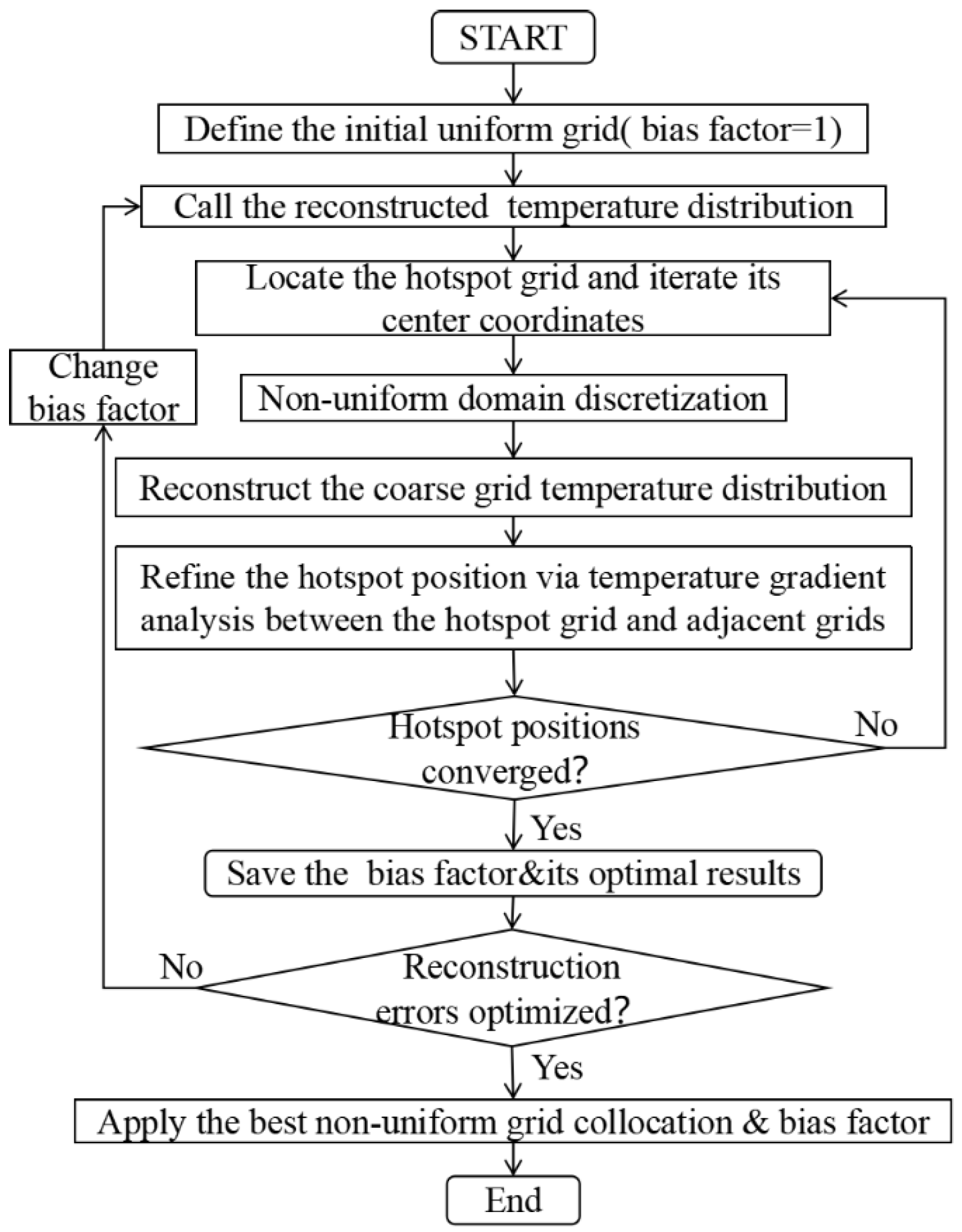
The flow chart of the AGES method is shown in Figure 4. Inspired by the CFD simulation in which refined meshes are employed for modelling complex parts to achieve enhanced results, local mesh refinement for hotspot regions is considered in the adaptive nonuniform domain discretization. Specifically, the SMS method is employed to identify and refine the center position of the hotspot grid, the nonuniform domain discretization is implemented, and then the inverse problem of acoustic pyrometry is solved. In addition, the AGES sets the starting point of the nonuniform discretization to the hotspot grid. This nonuniform discretization is consistent with the intrinsic gradient of the temperature field. The reconstruction errors serve as the evaluation criterion, and the hotspot grid location and nonuniform discretization parameters are optimized through an iterative selection process. In summary, AGES employs a dual-action strategy, which gives local refinement of grids near identified hotspots and sparse meshing across thermally uniform regions without increasing the total grid number.

2.3.3. AGES-AHK Method

In this research, a novel temperature reconstruction method based on the adaptive hybrid kernel and the adaptive grid evolution strategy is proposed and demonstrated. The proposed AGES-AHK method implements adaptive kernel adjustments on AGES-optimized nonuniform grids, integrating the optimization of AHK and AGES.
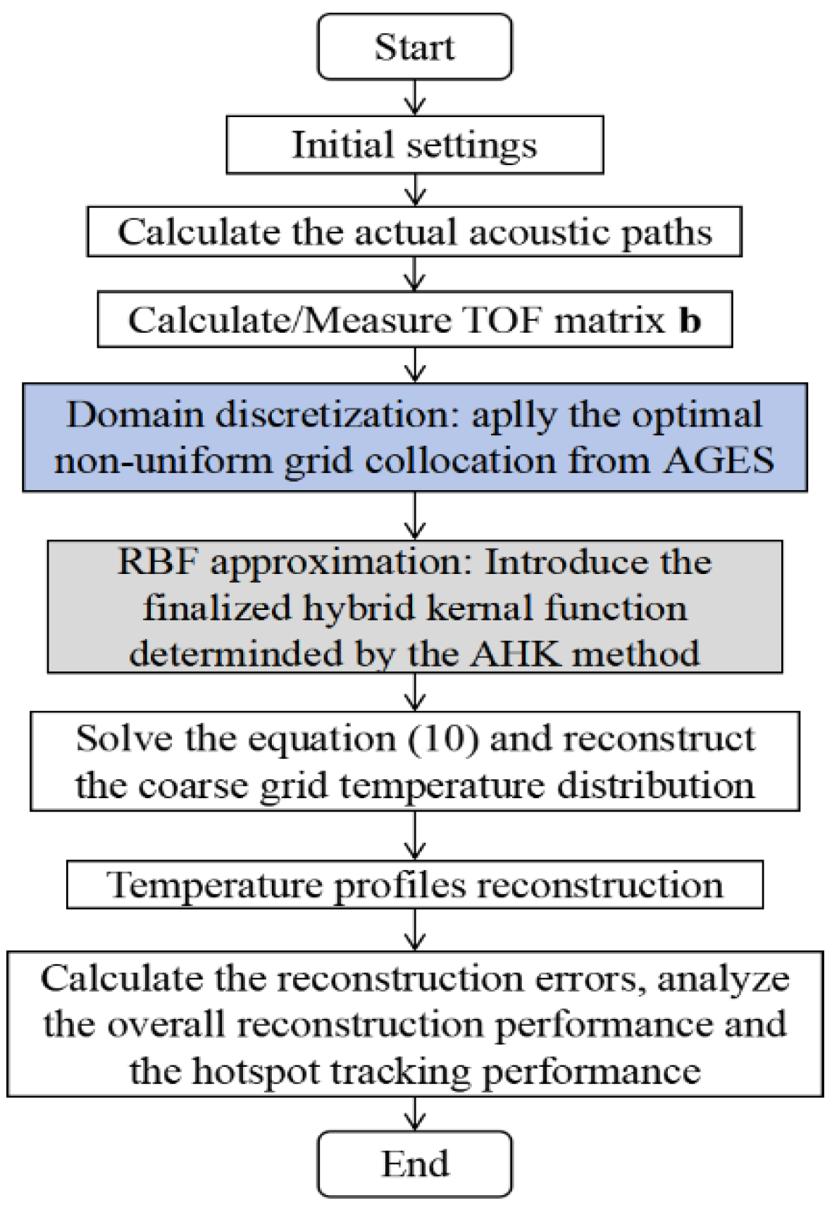
The flow chart of the AGES-AHK method and the complete reconstruction process are shown in Figure 5. Firstly, the acoustic path curve within the ROI is obtained by utilizing the known preset temperature phantom. The reciprocal of sound velocity matrix x is obtained from Equation (1) and the TOF matrix b can be derived from simulations or measurements.
Secondly, the adaptive nonuniform grid collocation is determined by AGES. By implementing adaptive nonuniform meshing without increasing the total grid number, AGES pre-optimizes grid density distribution to match the temperature field topography, thereby facilitating improvement in the reconstruction performance.
Thirdly, the RBF approximation with hybrid kernels is introduced to expand the reciprocal of sound velocity f in Equation (3). The finalized hybrid kernel function from the AHK method combines the sharp spatial localization characteristics of G with the global characterization of MQ, recovering the null-space component and reducing the ill-conditioned nature of the problem.
Next, the ill-conditioned linear equations = b in Equation (10) are solved by the reconstruction algorithm, thereby reconstructing the average grid temperature within the ROI and subsequently reproducing the continuous temperature profiles. Finally, the reconstruction errors are calculated to analyze the overall reconstruction performance and the hotspot tracking performance.
To assess the real-time applicability of the AGES-AHK method, it is important to evaluate its computational complexity. The overall computation of the AGES-AHK method is primarily influenced by the iterative nature of the adaptive hybrid kernel and grid evolution strategy. For a typical problem with n × n grids, the method requires several iterations for kernel adaptation and mesh refinement, resulting in increased complexity for grid-based reconstructions [28,29,30]. However, the adaptive nature of the algorithm reduces the need for exhaustive calculations across all regions, leading to enhanced efficiency compared to standard approaches. Additionally, optimization of the grid evolution strategy allows the method to focus computational resources on hotspot regions, thereby enhancing real-time applicability. Compared to traditional methods [11,25,26,27] with high computational costs, the AGES-AHK method strikes a balance between reconstruction accuracy and computational efficiency, making it suitable for real-time applications in industrial settings.

3. Results and Discussion

3.1. Initial Settings

According to previous studies, the least square QR decomposition (LSQR) algorithm has universal and comprehensive reconstruction performance [18,19,20,21], and requires far less time for parameter selection compared to Tikhonov regularization iterative methods and the truncated singular value decomposition regularization (TSVD) algorithm [1,16]. Consequently, the LSQR algorithm serves as the base algorithm for reconstruction in this study. Since LSQR is a generalized algorithm, a detailed description is not provided here.
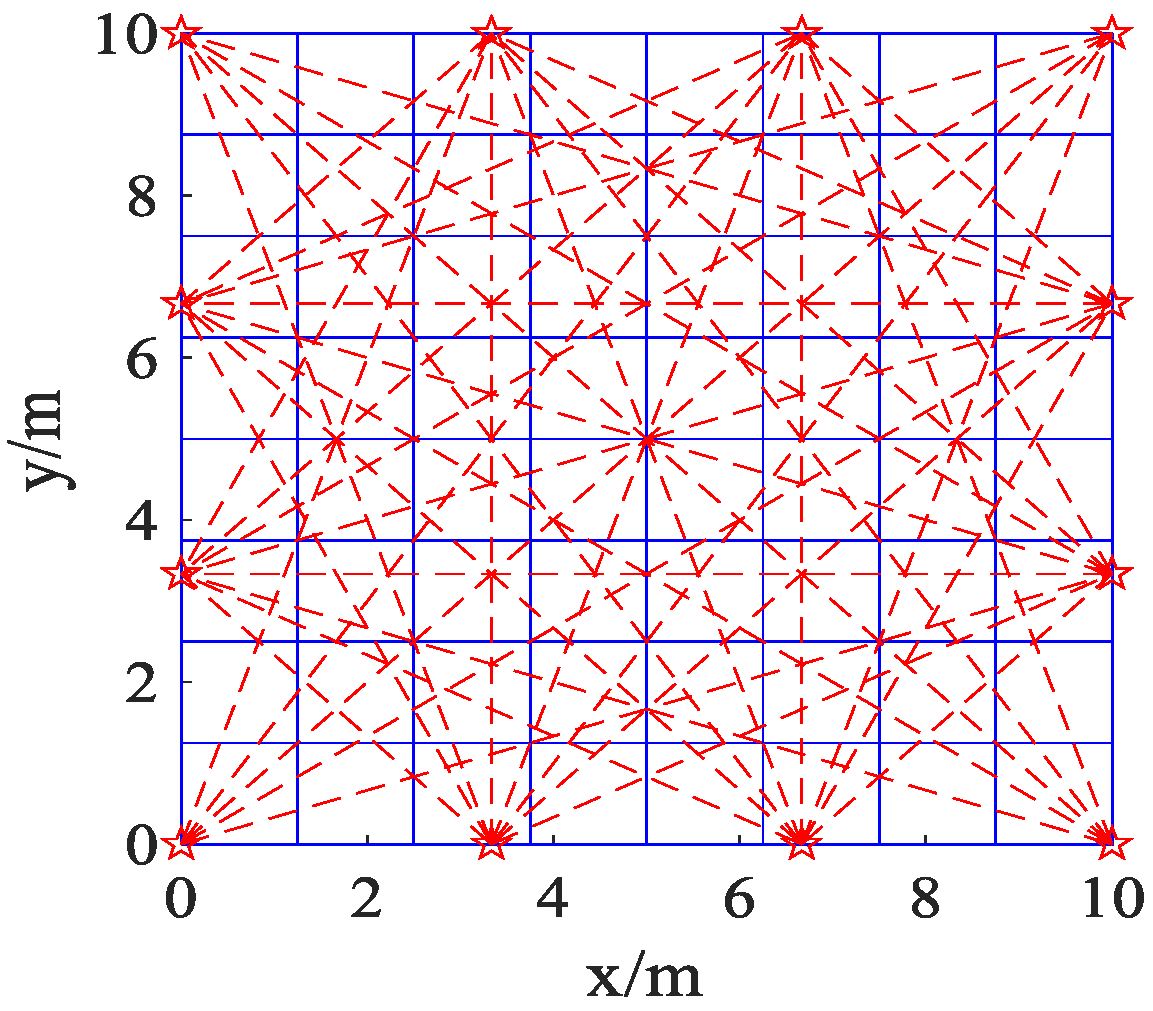
A classical layout scheme [14] was used in the research on two-dimensional acoustic reconstruction, as shown in the descriptive diagram in Figure 6. The ROI is a 10-m square that is equally divided into N = n × n grids (small blue squares). The ROI predefines the location of twelve acoustic transducers (red pentagrams), which are evenly spaced along the four boundaries of the ROI, to ensure that the acoustic paths between the acoustic transceivers cover the entire ROI in a more complete way. Considering the engineering limitations, the number of installed acoustic transducers is restricted. Twelve transceivers and a greater number of grids were chosen for better data density, uniformity, accuracy, resolution, and field-wide distribution.
The preset two-dimensional temperature phantom in the ROI is denoted as T(x, y). After the reconstruction, the results were compared with the preset true values and analyzed. The acoustic refraction effect was taken into account and the actual acoustic path curves were calculated for the construction of the coefficient matrix A in Equation (3).
The simulation data used in this study were generated based on predefined temperature phantom models rather than real experimental measurements. And the simulation data were generated as follows:
Initially, the preset temperature field and the ROI configurations are known. The acoustic path curve within the ROI is calculated from Equation (4), resulting in the acquisition of the coefficient matrix A. The TOF matrix b can then be derived through Equation (2). Subsequently, the ill-conditioned linear equation Ax = b in Equation (3) is solved, thereby reconstructing the average grid temperature within the ROI.
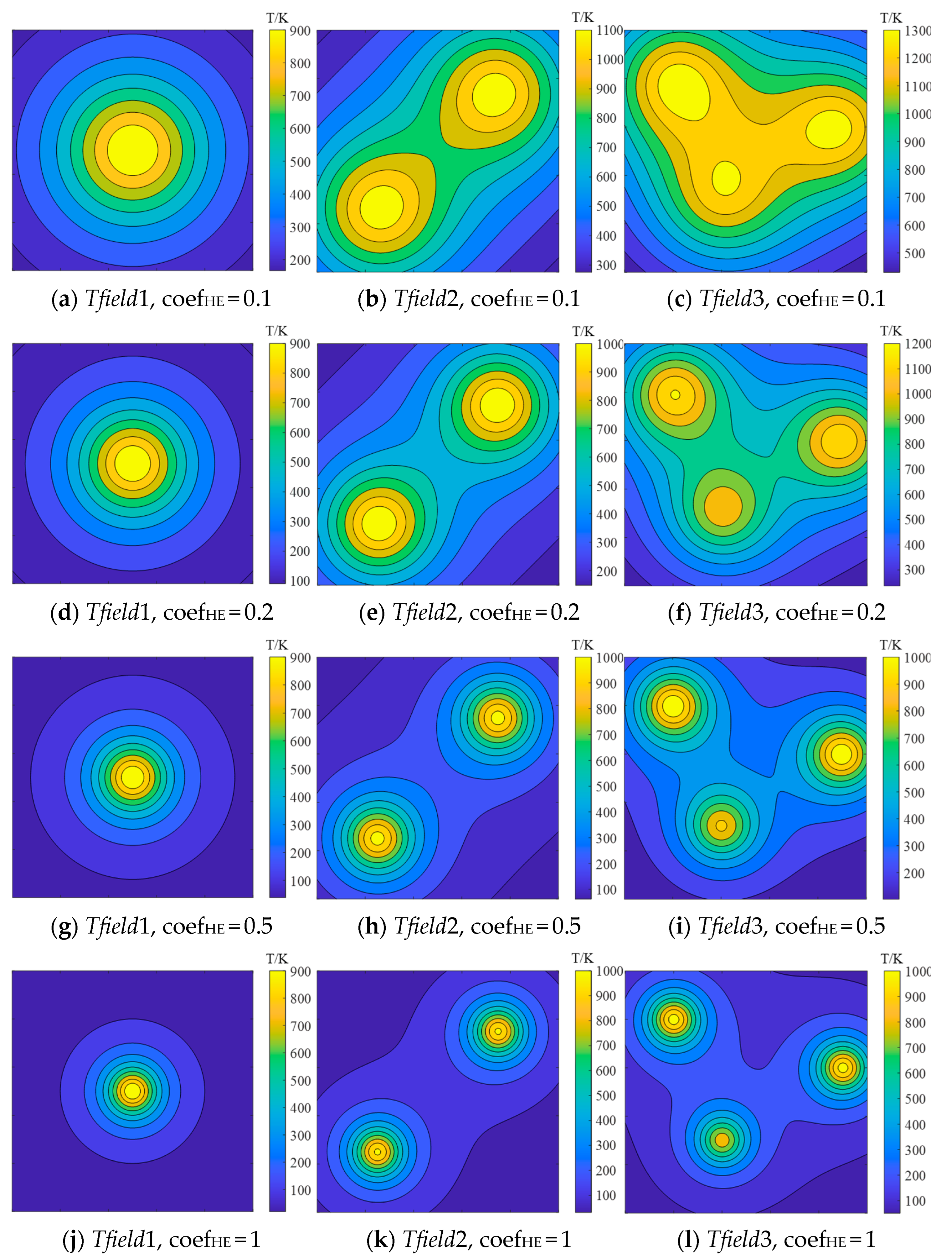
To investigate the effect of the intrinsic characteristics of the reconstructed temperature field (CHE) on reconstruction fidelity, three temperature phantoms of varying complexity were selected for reconstruction, namely single-peak symmetric Tfield1, double-peak symmetric Tfield2 and triple-peak asymmetric Tfield3. The selected temperature phantoms are the results of placing several ideal inverse-quadratic heat sources at different locations within a two-dimensional space, as described in:
T f i e l d 1 = 1000 coe f HE ( ( x 5 ) 2 + ( y 5 ) 2 ) + 1 T f i e l d 2 = 1000 coe f HE ( ( x 2.5 ) 2 + ( y 2.5 ) 2 ) + 1 + 1000 coe f HE ( ( x 7.5 ) 2 + ( y 7.5 ) 2 ) + 1 T f i e l d 3 = 1000 coe f HE ( ( x 2 ) 2 + ( y 8 ) 2 ) + 1 + 1000 coe f HE ( ( x 9 ) 2 + ( y 6 ) 2 ) + 1 + 800 coe f HE ( ( x 4 ) 2 + ( y 3 ) 2 ) + 1
where coefHE is a subfactor of the coefficient of the heating effect in the temperature fields, taken as 0.1, 0.2, 0.5 and 1. Altering the coefHE can easily modify both the heat source influence range and the gradient of the temperature phantom. A coefHE of 0.05 is commonly used by many researchers to conduct AT simulations [14,34,46,48].
Within the ROI, the temperature contour maps of the three temperature phantoms under four coefHE values are shown in Figure 7, and their corresponding CHE values are presented in Table 1.
As illustrated in Figure 7, when coefHE increases, the temperature attenuates faster with distance and the temperature distribution becomes more concentrated in space. Conversely, lower coefHE values yield flatter temperature profiles with broader thermal source coverage. Furthermore, coefHE modulates the diffusion and superposition effects of each source. Higher coefHE values results in more pronounced localized high-temperature zones, with strong heat source independence, weaker superposition effects, and high-temperature zones confined to the center of each source. Conversely, lower coefHE values lead to a more uniform temperature distribution and more pronounced interactions between the sources.
As shown in Table 1, there is a close linear relationship between the CHE of the temperature phantoms and coefHE. The CHE does not exceed 6.51 for coefHE values of 0.1 and 0.2. However, when coefHE is set at 0.5 and 1, the CHE increases significantly to high levels of 15 and 30, respectively.
When the reconstruction for three types of temperature phantoms is completed, qualitative and quantitative analyses are performed to evaluate the reconstruction performance. Multicriteria error analysis is used to evaluate the reconstruction accuracy. The normalized root mean square error (NRMSE) is utilized as the comprehensive description of the reconstruction fields, as described in Equation (13).
NRMSE = 1 N ( T r T a ) 2 / 1 N T a 2
where N is the number of grids. Tr and Ta are the reconstructed and actual grid average temperature, respectively.
The NRMSE normalizes the error metric to the scale of the observed data, which allows direct comparison of model performance and immediate understanding of error magnitude relative to data scale. Therefore, the NRMSE is used as a key performance metric to evaluate the overall reconstruction accuracy of temperature fields.
For hotspot tracking, the hotspot temperature error Eh and the hotspot position deviation Dh are given as:
E h = T R h T M h T M h , D h = ( x R h x M h ) 2 + ( y R h y M h ) 2 S R O I
where TMh and TRh are the temperature values of hotspots in the model phantom and the reconstructed temperature field, respectively. (xMh, yMh) and (xRh, yRh) are the 2D coordinates of hotspots in the model phantom and the reconstructed temperature field, respectively. SROI is the area of the region of interest.

3.2. Parametric Investigation of the Initial Reconstruction Result

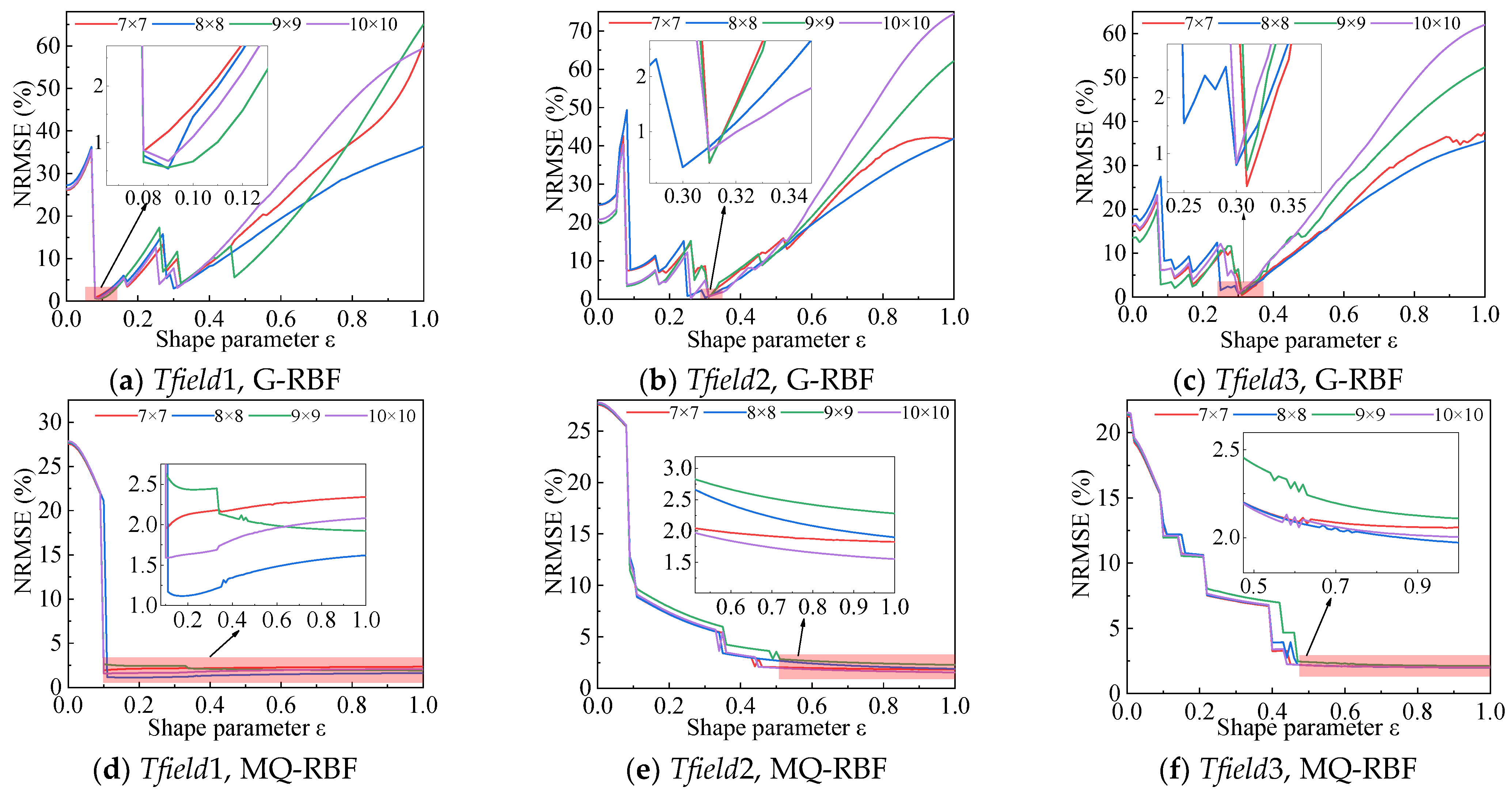
The accuracy of the reconstructed field is affected [16] by the selection of grid collocation, shape parameter ε and RBF types, etc. Using the simulation settings in Section 3.1 and a uniform grid collocation of n × n (n = 7–10), the coefHE of 0.1 was selected and three temperature phantoms in Equation (12) were reconstructed. Furthermore, G and MQ in Equation (8) were chosen with 501 shape parameters equally spaced between 0 and 1. The NRMSE was exclusively employed to evaluate the overall reconstruction error during the research process. The NRMSEs of the reconstructed temperature field under different conditions are shown in Figure 8, and the optimal parameters can be determined using the results obtained.
The trend of the variation in the reconstruction error with different shape parameters for two distinct RBF types is displayed in Figure 8. The overall trend of the reconstruction error does not significantly change with different grids, but the NRMSE varies greatly with the shape parameters.
The effect of the shape parameter ε on the reconstruction results has been investigated, and the NRMSE is critically influenced by the RBF type and shape parameters [49,50,51], as demonstrated in Figure 8 For the G-RBF, the NRMSE can be less than 1% at the optimal ε in the preset temperature phantoms. However, the G-RBF has a limited optimal ε range of approximately 0.1 in Tfield1 and 0.3 in Tfield2 and Tfield3, as demonstrated in Figure 8a–c. This is attributed to the fact that Tfield1 possesses the simplest single-peak structure, devoid of the influence of other heat sources, and consequently can be fitted with the sharper G-RBF. Conversely, Tfield2 and Tfield3 exhibit a more intricate structure characterized by interactions among heat sources, necessitating the use of a less sharp G-RBF for adequate fitting. In contrast, the MQ-RBF exhibits a wider range of optimal ε values than G-RBF, and reaches a stable low NRMSE value when ε approaches 1, with the lowest NRMSE stabilizing at 2%, as shown in Figure 8d–f.
In summary, the MQ-RBF exhibits a wide range of optimal ε values and good global characterization. Therefore, based on preliminary experiments and parametric investigation, the MQ-RBF with ε set to 1 was utilized as the basis method in this paper.
Next, the three temperature phantoms at coefHE = 0.1 were reconstructed with a uniform grid collocation of n × n (n = 7–19) using the basis method, and their reconstruction performances are shown in Figure 9.
As shown in Figure 9, the NRMSEs fluctuate downward as the number of grids increases. When the number of grids increases to a certain extent, the NRMSE tends to converge. Increasing the number of grids provides a more detailed description of the reconstructed field and reduces the error. However, owing to the nature of the ill-posed problem, obtaining an unbiased estimator of the true value is impossible. With the increase in the number of grids, as does the increase in the number of unknown parameters, the problem’s ill-conditioned nature then exacerbates, which results in an increase in the reconstruction error. Due to the combined effects above, the NRMSE shows a much smaller variation amplitude when the number of grids increases to a certain extent, indicating that increasing the number of grids appropriately is advantageous.
Another metric of reconstruction performance is computation time. 200 operations were performed under the same computer conditions to obtain the average total computation time of the basis method. As illustrated in Figure 9, the total computation time increases exponentially as the number of grids increases, with a significant jump at n = 12.
Considering the effect of grid configuration on the total computation time and reconstruction accuracy, a uniform grid configuration of 11 × 11 was selected as a trade-off in the basis method for the subsequent study in this paper, as shown in the red box in Figure 9.

3.3. The Reconstruction Results of the AGES-AHK Method

The reconstruction results of the finalized AGES-AHK method is shown in Table 2.
The coefficient of heating effect in Equation (12) is a critical parameter that affects the gradient and the complexity of the temperature phantoms. As shown in Table 2, the NRMSE and Eh exhibit a marked increase with elevated coefHE values in the three temperature phantoms. It can be contributed to the fact that, with the increase of coefHE, the temperature distribution becomes more concentrated in localized high-temperature regions, making it more challenging to accurately reconstruct the temperature field.
In all three temperature phantoms, the AGES-AHK method achieves a maximum Dh of less than 3% and NRMSE values below 6.7%, representing the optimal performance in hotspot position tracking and overall reconstruction. At coefHE values of 0.1, 0.2, and 0.5, the NRMSE is less than 3.7% and Eh is less than 15%, representing the superior overall reconstruction performance and peak temperature tracking ability of AGES-AHK method. Even at the highest coefHE value of 1, the AGES-AHK method was still able to obtain meaningful results under extreme conditions.
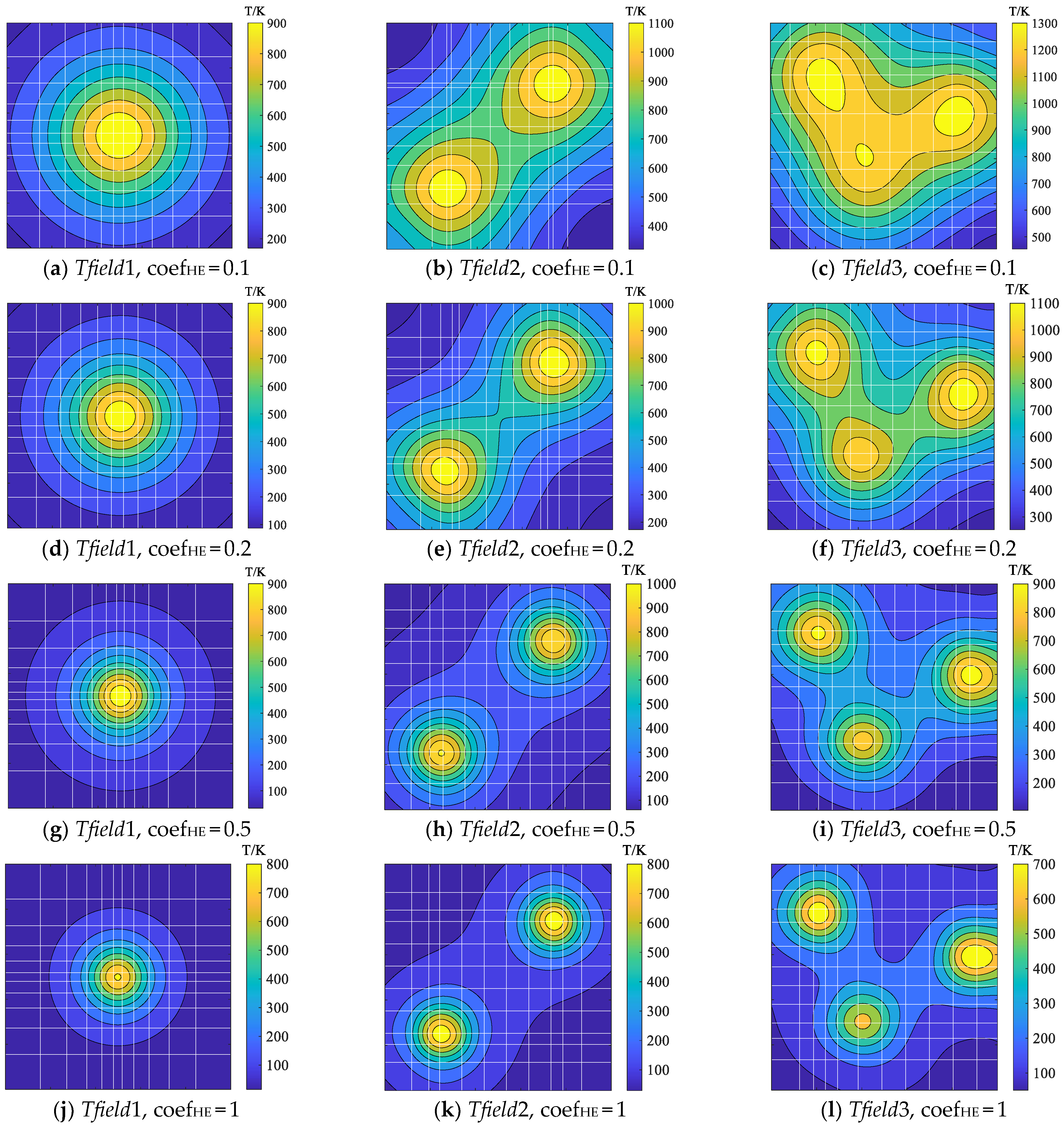
The temperature contour maps reconstructed by the finalized AGES-AHK method is shown in Figure 10.
As illustrated in Figure 10, when the coefHE value is low, the temperature distribution of the reconstructed field is relatively uniform, and the interactions between the heat sources are pronounced. Conversely, when coefHE increases, the reconstructed temperature attenuates faster with distance, and the temperature distribution is more concentrated in space. Furthermore, higher coefHE values results in more pronounced localized high-temperature zones, with strong heat source independence, weaker superposition effects, and high-temperature zones confined to the center of each source. The nature of this temperature distribution, which changes with coefHE, is consistent with the theoretical temperature phantoms in Figure 7.
In comparison to the theoretical temperature phantoms in Figure 7, the AGES-AHK reconstructed temperature contour maps in Figure 10 shows an extremely high reproduction performance. At coefHE values of 0.1, 0.2 and 0.5, the reconstructed results of the AGES-AHK method can accurately reproduce the overall temperature field topography, the extent of the hot zone, the location of hotspots, the peak temperature and the overall temperature range. In the extreme case of coefHE = 1, AGES-AHK is able to reproduce the overall temperature field topography, the extent of the hot zone, and qualitatively track the location of hotspots and the peak temperature well. These results illustrate the validity of the AGES-AHK method.
As shown in Figure 10, the white lines represent the nonuniform discretization of AGES, which is in accordance with the intrinsic gradient of the theoretical temperature field. In the domain discretization of all three temperature phantoms, AGES gives local refinement of grids near identified hotspots and sparse meshing across thermally uniform regions. This improves the resolution of grid reconstruction in the vicinity of the identified hotspot, whereas in larger grids, the reconstruction results are overaveraged, thus relatively reducing the reconstruction error. It is noteworthy that markedly nonuniform grid collocations are exhibited in Tfield1, whereas the smallest grid precisely encloses the theoretical hotspot.
In summary, the proposed AGES-AHK method shows great improvement compared to previous studies [25,26,30,36,38]. The AHK method combines the sharp spatial localization characteristics of G with the global characterization of MQ, thereby enhancing the suitability for reconstructing large-gradient temperature fields [26,36,38], as evidenced by Table 2. The AGES method modifies the grid density distribution to match the temperature field topography at a finite number of measurement points, improving the fixed-center non-uniform distribution [30] and the spatial moving of hexagonal grids [25], as evidenced by Figure 10.

3.4. The Discussion of the Overall Reconstruction Error and the Hotspot Tracking Performance

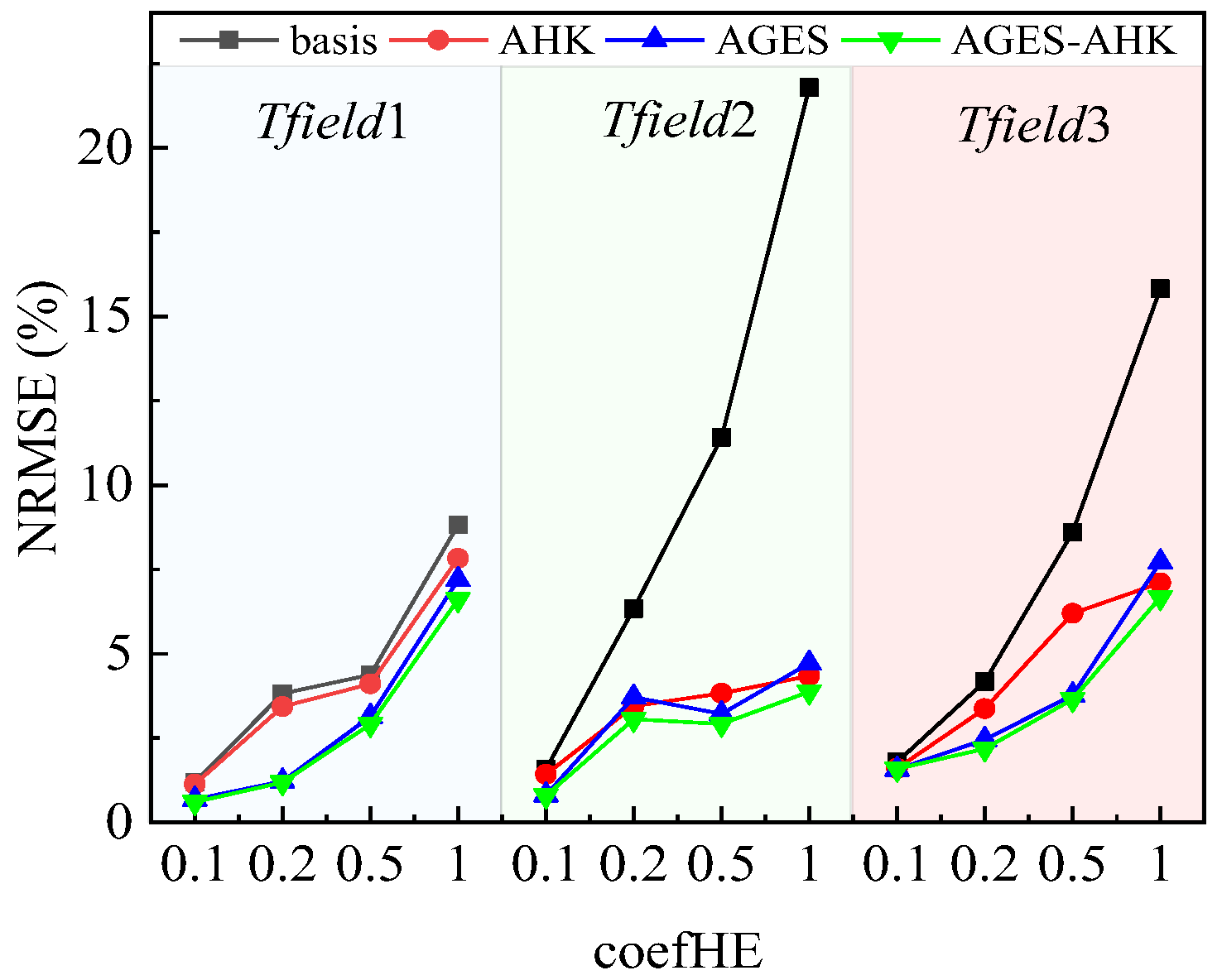
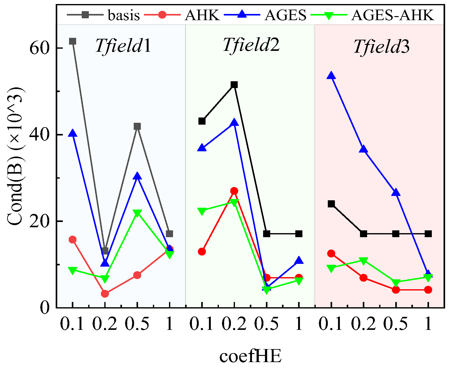
Subsequently, the basis method, the AHK method, the AGES and the AGES-AHK method were used to reconstruct the three temperature phantoms under four coefHE values, and a quantitative analysis was conducted. The overall reconstruction error and the condition number of coefficient matrix B (denoted as Cond(B)) are shown in Figure 11 and Figure 12, respectively. The hotspot tracking performance is represented by the hotspot temperature error and the hotspot position deviation. The hotspot temperature error Eh is shown in Figure 13. And the hotspot position deviation Dh is shown in Table 3, Table 4 and Table 5.
As shown in Figure 11, the NRMSE of all four methods exhibits a marked increase with elevated coefHE values in the three temperature phantoms, verifying the effect of the intrinsic characteristics of the reconstructed temperature field on the difficulty of reconstruction.
For the basis method, when coefHE values were maintained at 0.1 and 0.2, all three temperature phantoms exhibited relatively uniform temperature distributions with NRMSE values below 7%, indicating good reconstruction performance. However, at coefHE values of 0.5 and 1, these phantoms demonstrated a sharp escalation in temperature gradients accompanied by a significant NRMSE increase.
The implementation of both AHK and AGES effectively reduced the NRMSE across all twelve cases compared to the basis method. AGES demonstrated superior NRMSE reduction capability over the AHK method under coefHE conditions of 0.1, 0.2, and 0.5. Notably, the two methodologies exhibited comparable efficacy at coefHE = 1.
Ultimately, the integrated AGES-AHK method achieved the optimal overall reconstruction performance, with NRMSE less than 6.7%. As demonstrated in Figure 11, the AGES-AHK method exhibits the lowest NRMSE, improving reconstruction accuracy by more than 33% compared to the basis method (traditional LSQR algorithm, incorporated with MQ-RBF approximation and uniform domain discretization).
Figure 12 shows the condition number of the coefficient matrix B of Equation (10) (Cond(B)) for the four reconstruction methods. Cond(B) is directly related to the ill-conditioned nature of the AP problem. An increasing Cond(B) indicates the exacerbating ill-conditioned nature of Equation (10) and the increased reconstruction difficulty.
As shown in Figure 12, the implementation of AHK substantially reduces Cond(B) across all three temperature phantoms. This suggests that modifications to the kernel function through AHK effectively mitigate the ill-conditioned nature of Equation (10), thereby enhancing reconstruction accuracy and reducing the NRMSE.
The implementation of AGES reduces Cond(B) in Tfield1 and Tfield2, which reduces the ill-conditioned nature of the problem and thus improves the reconstruction performance. However, for Tfield3, the implementation of AGES increases Cond(B) to varying degrees, thereby exacerbating the ill-conditioned nature of the problem. Conversely, the reconstruction error still decreases to varying degrees. As shown in Figure 11, AGES demonstrated superior NRMSE reduction capabilities over AHK. This can be attributed to the fact that AGES employs a dual-action strategy, which gives local refinement of grids near identified hotspots and sparse meshing across thermally uniform regions, thereby pre-optimizing grid density distribution to match the temperature field topography. This bidirectional optimization outperforms AHK’s unidirectional kernel adjustment in reducing NRMSE. It can thus be concluded that the AGES pre-fits the temperature field from the meshing perspective, thereby facilitating improvement in the reconstruction performance. And this positive effect clearly overwhelms the negative effect of the increased ill-conditioned nature of the problem.
The AGES-AHK method implements adaptive kernel adjustments on AGES-optimized nonuniform grids, integrating the optimization of AHK. As shown in Figure 12, AGES-AHK reduces the Cond(B) across all temperature phantoms compared to standalone AGES or the basis method. This reduction directly translates to mitigating the ill-conditioned nature of the AP problem, especially in regions with high temperature gradients, thereby effectively reducing the reconstruction difficulty and errors.
As shown in Figure 13, the hotspot temperature error Eh of all four methods exhibits a progressive increase with elevated coefHE values in the three temperature phantoms, indicating an exacerbation of the hotspot peak temperature tracking performance. Once again, the effect of the intrinsic characteristics of the reconstructed temperature field on the difficulty of reconstruction is verified through simulation.
A comparative analysis with the basis method reveals that both the AGES and AHK methods effectively reduce Eh across all three temperature phantoms. Notably, AGES demonstrates superior Eh reduction compared to the AHK method. This discrepancy arises because the AHK method exclusively reduces Cond(B) through kernel function modifications, thereby alleviating the ill-conditioned nature of Equation (10) and enhancing the overall reconstruction accuracy. However, since AHK does not alter the uniform mesh discretization, the inherent limitation of the domain discretization assumption remains unaddressed. The observed Eh reduction of AHK is a secondary effect of its NRMSE reduction.
In contrast to AHK, AGES gives local refinement of grids near identified hotspots, as shown in Figure 10. Consequently, the hotspot grids in the final mesh configurations feature are significantly smaller than the initial uniform grids, and the hotspot temperature values are corrected by averaging the refined grids in its vicinity, leading to a substantial reduction of Eh.
Then, the AGES-AHK method combines the advantages of AGES and AHK to achieve the best hotspot temperature tracking performance with Eh values considerably lower than those of the basis method. At coefHE values of 0.1, 0.2, and 0.5, the maximum Eh of Tfield1, Tfield2, and Tfield3 does not exceed 2.5%, 5% and 15%, respectively. Even at the highest coefHE value of 1, the maximum Eh of the three temperature phantoms is less than 25%, significantly lower than the basis method.
Another important criterion for hotspot tracking performance is the hotspot position deviation Dh. As shown in Table 3, Tfield1 exhibits Dh = 0 across all 12 cases due to its inherent high symmetry. Similarly, Table 4 reveals that Tfield2 maintains Dh < 1.41% at coefHE = 0.1 and 0.2, with Dh collapsing to 0 at coefHE = 0.5 and 1, a consequence of its symmetric configuration. Critically, the proposed AGES and AHK methods fail to achieve meaningful Dh reduction in either Tfield1 or Tfield2. This limitation arises because the intrinsic symmetry of these phantoms inherently minimizes localization errors, leaving minimal margin for algorithmic improvement.
In contrast, the highly asymmetric temperature phantom Tfield3 exhibits markedly divergent responses to AGES and AHK methods regarding Dh, as quantitatively validated in Table 5. The AHK method fails to meaningfully reduce Dh because AHK does not alter the fundamental uniform domain discretization scheme. Consequently, the inherent limitation of the domain discretization assumption—which obscures continuous temperature variations within individual grids—remains unaddressed. Conversely, AGES demonstrates superior Dh performance than that of the basis method and the AHK method. This is because AGES is iterated with the grid in which the hotspot is located. The hotspot grids in the final mesh configurations feature are significantly smaller than the initial uniform grids. Then hotspot positions are refined via temperature gradient analysis between nonuniform hotspot grids and adjacent regions, which leads to a decrease in Dh.
The finalized AGES-AHK method integrates the benefits of AGES and AHK. In all three temperature phantoms, the AGES-AHK method achieves an average Dh of less than 2.14% and a maximum Dh of less than 3%, representing the optimal performance in hotspot position tracking, as evidenced by Table 5.

3.5. The Discussion of the Practical Challenges and Future Advancements

In practical application scenarios, the AGES-AHK method may encounter challenges such as sensitivity to measurement noise, the tuning of key parameters, and the transition to three-dimensional domains.
In real-world applications, noise can introduce errors in time-of-flight measurements, resulting in inaccuracies especially in high-gradient regions where the temperature distribution is more sensitive to small changes in data.
In the preliminary work of this study, the effect of noise on reconstruction had been analyzed. The results show that NRMSE grows approximately linearly with increasing random noise. Adding a ±1% TOF error increases the average NRMSE by more than 0.4%, which is a sizable increase. This is because the AGES-AHK method is a reallocation of computational resources without altering the underlying reconstruction algorithm LSQR, meaning the method’s anti-noise performance is not inherently improved.
In future work, implementing noise reduction techniques (e.g., Kalman Filtering) to reduce random noise and regularization techniques (e.g., Tikhonov) to modify the reconstruction algorithm could help reduce the impact of noise on reconstruction accuracy.
Furthermore, the AGES-AHK method’s performance is highly dependent on the tuning of key parameters, including the hybrid kernel shape parameters and the adaptive grid density in nonuniform discretization. Future work could focus on exploring adaptive methods for parameter tuning.
Regarding the dependence on parameter tuning, it is essential to establish a customized parameter library for the target application scenarios through a large number of simulations and experiments. Through this approach, the appropriate parameter base values can be quickly selected within the scope of the application scenario. The optimal parameter values can then be obtained with slight modifications. This parameter library is similar to the common methods in industrial applications, which would not only enhance efficiency but also make the method more accessible for real-world applications.
The results in this study demonstrate the effectiveness of the AGES-AHK method in 2D applications. However, extending AGES-AHK to 3D would increase computational costs cubically (O(n3) grids vs. O(n2)) due to refined meshing and acoustic path calculations. Critical variables affecting performance and accuracy in 3D include the number of transducers, the grid resolution, and the size of the ROI and heat sources. GPU acceleration or parallelized LSQR solvers could mitigate these costs.
Additionally, the AGES and AHK methods may face challenges in scenarios with highly nonlinear thermal gradients or irregular temperature distributions.
By modifying the grid density distribution to match the temperature field topography, AGES essentially constitutes a trade-off for reallocating computational resources with limited measurement points and grids. In cases where temperature fields exhibit highly irregular or chaotic variations, the reliance on adaptive grid evolution may result in the missing of broader trends. Furthermore, the nonuniform discretization may fail to capture fine details in regions with rapid, non-continuous changes. These limitations highlight the necessity for the integration of higher-order interpolation methods or machine learning techniques to predict optimal grid placements.
The finalized adaptive hybrid kernel from the AHK method combines the sharp spatial localization characteristics of G with the global characterization of MQ. However, the Gaussian kernel may fail to fit temperature profiles with drastically excessive gradients or capture the complex interactions among high-gradient regions. The MQ kernel, while showing good global characterization, may fail to capture the broad trends of the reconstruction field in cases where temperature fields exhibit highly irregular or chaotic variations. In future research, adaptations of the AHK method could include the use of more flexible kernel functions or machine learning techniques to better accommodate irregular or nonlinear thermal distributions.

4. Conclusions

In this research, a novel reconstruction method for acoustic pyrometry dedicated for strong temperature gradients and limited measurement points is proposed and demonstrated. Based on the qualitative and quantitative analyses of the reconstruction results, the following conclusions can be drawn:
(1)
The effect of the intrinsic characteristics of the reconstructed temperature field (CHE) on the difficulty of reconstruction is verified through literature reviews and reconstruction results.
(2)
The finalized adaptive hybrid kernel from the AHK method combines the sharp spatial localization characteristics of G with the global characterization of MQ, thereby alleviating the ill-conditioned nature of the problem and enhancing the suitability for reconstructing large-gradient temperature fields.
(3)
By implementing adaptive nonuniform meshing without increasing the total grid number, AGES pre-optimizes grid density distribution to match the temperature field topography, thereby facilitating improvement in the reconstruction performance.
(4)
The finalized AGES-AHK method integrates the optimization of AHK and AGES, achieving significant improvements over basis data in both reconstruction fidelity and hotspot characterization. At CHE levels below 15, the AGES-AHK method achieved the lowest NRMSE of less than 3.7%, Eh of less than 15% and Dh of less than 2.24%, representing its superior overall reconstruction performance and hotspot tracking ability. Even at the highest CHE level of 30, the AGES-AHK method was still able to reproduce the overall temperature field topography and qualitatively track the hotspots.
These conclusions have important implications for furnace temperature monitoring, combustion control, environmental protection and energy saving. One promising direction is the further improvement of discretization methods, particularly for highly irregular temperature fields. Exploring alternative mesh refinement techniques and hybrid kernel functions, such as incorporating the use of machine learning-based predictions of temperature gradients, could enhance grid evolution strategies and flexible kernel functions. Additionally, implementing noise reduction techniques and regularization techniques in the reconstruction process could help improve the reconstruction robustness. Furthermore, incorporating additional information or constraints in combination with our proposed methodology could further improve reconstruction performance under extreme conditions. These advancements would enable more widespread application of the AGES-AHK method in industrial settings for better prospects.

Author Contributions

J.T.: conceptualization, methodology, validation, software, writing—original draft preparation. L.C.: writing—original draft preparation, visualization. N.L.: supervision, project administration, funding acquisition, writing—review and editing. Q.Z.: conceptualization, supervision, formal analysis. Z.G.: visualization, supervision, funding acquisition. J.Z.: resources, funding acquisition, investigation, data curation. All authors have read and agreed to the published version of the manuscript.

Funding

This research was funded by the National Key Laboratory of Aerospace Liquid Propulsion Fund (No. HTKJ2023KL011007).

Institutional Review Board Statement

Not applicable.

Informed Consent Statement

Not applicable.

Data Availability Statement

The original contributions presented in this study are included in the article. Further inquiries can be directed to the corresponding author.

Conflicts of Interest

The authors declare no conflicts of interest.

References

  1. Zhang, S.; Shen, G.; An, L.; Niu, Y. Online monitoring of the two-dimensional temperature field in a boiler furnace based on acoustic computed tomography. Appl. Therm. Eng. 2015, 75, 958–966. [Google Scholar] [CrossRef]
  2. FAN, B.; SHEN, C.; WANG, K. Simulation on spray combustion flow field of the air heater. J. Rocket Propuls. 2023, 49, 13–22. [Google Scholar]
  3. Bramanti, M.; Salerno, E.A.; Tonazzini, A.; Pasini, S.; Gray, A. An acoustic pyrometer system for tomographic thermal imaging in power plant boilers. IEEE Trans. Instrum. Meas. 1996, 45, 159–167. [Google Scholar] [CrossRef]
  4. Shen, X.; Xiong, Q.; Shi, X.; Wang, K.; Liang, S.; Gao, M. Ultrasonic temperature distribution reconstruction for circular area based on Markov radial basis approximation and singular value decomposition. Ultrasonics 2015, 62, 174–185. [Google Scholar] [CrossRef] [PubMed]
  5. Pan, G.; Niu, X.; Pan, L.; Zheng, M.; Sun, J.; Ding, Z. Analysis on outlet temperature uniformity of hydrogen/oxygen preburner with high-pressure and low-mixture-ratio. J. Rocket Propuls. 2023, 49, 29–35. [Google Scholar]
  6. Kong, Q.; Jiang, G.; Liu, Y.; Sun, J. 3D Temperature Distribution Reconstruction in Furnace Based on Acoustic Tomography. Math. Probl. Eng. 2019, 2019, 1830965. [Google Scholar] [CrossRef]
  7. Zhang, S.; Shen, G.; An, L.; Niu, Y.; Jiang, G. Monitoring ash fouling in power station boiler furnaces using acoustic pyrometry. Chem. Eng. Sci. 2015, 126, 216–223. [Google Scholar] [CrossRef]
  8. Tsai, W.-Y.; Chen, H.-C.; Liao, T.-L. High accuracy ultrasonic air temperature measurement using multi-frequency continuous wave. Sens. Actuators A Phys. 2006, 132, 526–532. [Google Scholar] [CrossRef]
  9. Liu, Y.; Liu, S.; Lei, J.; Liu, J.; Schlaberg, H.I.; Yan, Y. A method for simultaneous reconstruction of temperature and concentration distribution in gas mixtures based on acoustic tomography. Acoust. Phys. 2015, 61, 597–605. [Google Scholar] [CrossRef]
  10. Tsai, W.-Y.; Huang, C.-F.; Liao, T.-L. New implementation of high-precision and instant-response air thermometer by ultrasonic sensors. Sens. Actuators A Phys. 2005, 117, 88–94. [Google Scholar] [CrossRef]
  11. Liu, S.; Liu, S.; Ren, T. Acoustic Tomography Reconstruction Method for the Temperature Distribution Measurement. IEEE Trans. Instrum. Meas. 2017, 66, 1936–1945. [Google Scholar] [CrossRef]
  12. Xie, L.B.; Liu, T.; Zhang, Z.G.; Shao, W. 2-D temperature reconstruction based on the algorithm of interpolation and iterative. Proc. Chin. Soc. Electr. Eng. 2004, 24, 249–252. [Google Scholar]
  13. Andersen, A.; Kak, A.C. Simultaneous Algebraic Reconstruction Technique (SART): A Superior Implementation of the ART Algorithm. Ultrason. Imaging 1984, 6, 81–94. [Google Scholar] [CrossRef]
  14. Kong, Q.; Jiang, G.; Liu, Y.; Sun, J. 3D high-quality temperature-field reconstruction method in furnace based on acoustic tomography. Appl. Therm. Eng. 2020, 179, 115693. [Google Scholar] [CrossRef]
  15. Wang, R.; An, L.; Shen, G.; Zhang, S. Acoustic reconstruction of three-dimensional temperature field based on regularized SVD algorithm. Chin. J. Comput. Phys. 2015, 32, 195–201. [Google Scholar] [CrossRef]
  16. Zhang, J.; Qi, H.; Jiang, D.; He, M.; Ren, Y.; Su, M.; Cai, X. Acoustic tomography of two dimensional velocity field by using meshless radial basis function and modified Tikhonov regularization method. Measurement 2021, 175, 109107. [Google Scholar] [CrossRef]
  17. Zhang, J.; Qi, H.; Ren, Y.; Su, M.; Cai, X. Acoustic tomography of temperature and velocity fields by using the radial basis function and alternating direction method of multipliers. Int. J. Heat Mass Transf. 2022, 188, 122660. [Google Scholar] [CrossRef]
  18. Fan, W.; Chen, Y.; Pan, H.; Ye, Y.; Cai, Y.; Zhang, Z. Experimental study on underwater acoustic imaging of 2-D temperature distribution around hot springs on floor of Lake Qiezishan, China. Exp. Therm. Fluid Sci. 2010, 34, 1334–1345. [Google Scholar] [CrossRef]
  19. Yan, H.; Li, X.; Wang, S. Reconstruction of three dimensional temperature field based on least square method and Kriging interpolation. J. Shenyang Univ. Technol. 2014, 36, 303–307. [Google Scholar] [CrossRef]
  20. Shen, X.; Xiong, Q.; Shi, W.; Liang, S.; Shi, X.; Wang, K. A New Algorithm for Reconstructing Two-Dimensional Temperature Distribution by Ultrasonic Thermometry. Math. Probl. Eng. 2015, 2015, 1–10. [Google Scholar] [CrossRef]
  21. Lu, J.; Wakai, K.; Takahashi, S.; Shimizu, S. Acoustic computer tomographic pyrometry for two-dimensional measurement of gases taking into account the effect of refraction of sound wave paths. Meas. Sci. Technol. 2000, 11, 692. [Google Scholar] [CrossRef]
  22. Yan, H.; Chen, G.; Zhou, Y.; Liu, L. Primary study of temperature distribution measurement in stored grain based on acoustic tomography. Exp. Therm. Fluid Sci. 2012, 42, 55–63. [Google Scholar] [CrossRef]
  23. Zhang, S.; Shen, G.; An, L.; Li, G. Ash fouling monitoring based on acoustic pyrometry in boiler furnaces. Appl. Therm. Eng. 2015, 84, 74–81. [Google Scholar] [CrossRef]
  24. Kong, Q.; Jiang, G.; Liu, Y.; Sun, J. Location of the Leakage From a Simulated Water-Cooling Wall Tube Based on Acoustic Method and an Artificial Neural Network. IEEE Trans. Instrum. Meas. 2021, 70, 1–18. [Google Scholar] [CrossRef]
  25. Soma, P.; Fu-Sung, L.; Ching-Chuan, H.; Ya-Han, L.; Chen-Yuan, L.; Shan-Wen, D.; Chih-Hsien, H. An Acoustic Hotspot Tracking Algorithm for Highly Centralized Gas Temperature Distribution. IEEE Trans. Ultrason. Ferroelectr. Freq. Control 2020, 68, 1370. [Google Scholar] [CrossRef]
  26. Yu, Y.; Xiong, Q.; Li, Q.; Wu, C.; Wang, K.; Gao, M.; Liang, S. A method for ultrasound thermal image distribution reconstruction. Meas. Sci. Technol. 2019, 30, 095007. [Google Scholar] [CrossRef]
  27. Jia, R.; Xiong, Q.; Xu, G.; Wang, K.; Liang, S. A method for two-dimensional temperature field distribution reconstruction. Appl. Therm. Eng. 2017, 111, 961–967. [Google Scholar] [CrossRef]
  28. Yu, Y.; Xiong, Q.; Yang, M.; Wu, C.; Zhu, Q.; Wang, K.; Gao, M. Krylov Subspace Methods for Regularized Models in Acoustic Temperature Reconstruction from Simulated and Real Measurements. IEEE Trans. Instrum. Meas. 2021, 70, 9514111. [Google Scholar] [CrossRef]
  29. Yu, Y.; Xiong, Q.; Li, Q.; Wu, C.; Gao, M.; Wang, K. A hybrid kernel function approach for acoustic reconstruction of temperature distribution. Measurement 2020, 166, 108238. [Google Scholar] [CrossRef]
  30. Sreeram, B.; Chaitanya, S.K.; Jaswanth, K.K.A.; Srinivasan, K. Precise temperature reconstruction in acoustic pyrometry: Impact of domain discretization and transceiver count. Appl. Therm. Eng. 2024, 238, 122009. [Google Scholar] [CrossRef]
  31. Lifeng, Z.; Jing, L. Acoustic Tomography Temperature Reconstruction Based on Virtual Observation and Residual Network. IEEE Sens. J. 2022, 22, 17054–17064. [Google Scholar] [CrossRef]
  32. Ruixi, J.; Qingyu, X.; Shan, L. Acoustic imaging for temperature distribution reconstruction. AIP Adv. 2016, 6, 125018. [Google Scholar] [CrossRef]
  33. Sha, L.; Shi, L.; Guowei, T.; Guowei, T. Reconstruction method for inversion problems in an acoustic tomography based temperature distribution measurement. Meas. Sci. Technol. 2017, 28, 115005. [Google Scholar] [CrossRef]
  34. Qian, K.; Genshan, J.; Yuechao, L. Research on Temperature Field Reconstruction Based on RBF Approximation with Polynomial Reproduction Considering the Refraction Effect of Sound Wave Paths. Sound Vib. 2018, 52, 9–20. [Google Scholar] [CrossRef]
  35. Zhou, X.; Dong, C.; Zhao, C.; Bai, X. Temperature-field reconstruction algorithm based on reflected sigmoidal radial basis function and QR decomposition. Appl. Therm. Eng. 2020, 171, 114987. [Google Scholar] [CrossRef]
  36. Li, Z.; Xinzhi, Z.; Chenlong, D.; Yuhui, W.; Hailin, W. Ultrasonic Thermometry Algorithm Based on Inverse Quadratic Function. IEEE Trans. Ultrason. Ferroelectr. Freq. Control 2020, 68, 1876–1884. [Google Scholar] [CrossRef]
  37. Yuhui, W.; Xinzhi, Z.; Li, Z.; Chenlong, D.; Hailin, W. A Method for Reconstruction of Boiler Combustion Temperature Field Based on Acoustic Tomography. Math. Probl. Eng. 2021, 2021, 9922698. [Google Scholar] [CrossRef]
  38. Wang, H.; Zhou, X.; Yang, Q.; Chen, J.; Dong, C.; Zhao, L. A Reconstruction Method of Boiler Furnace Temperature Distribution Based on Acoustic Measurement. IEEE Trans. Instrum. Meas. 2021, 70, 9600413. [Google Scholar] [CrossRef]
  39. Zhang, J.; Qi, H.; Ji, Y.; Ren, Y.; He, M.; Su, M.; Cai, X. Nonlinear Acoustic Tomography for Measuring the Temperature and Velocity Fields by Using the Covariance Matrix Adaptation Evolution Strategy Algorithm. IEEE Trans. Instrum. Meas. 2022, 71, 4500214. [Google Scholar] [CrossRef]
  40. Aster, R.C.; Borchers, B.; Thurber, C.H. Chapter Three—Rank Deficiency and Ill-Conditioning. In Parameter Estimation and Inverse Problems, 3rd ed.; Aster, R.C., Borchers, B., Thurber, C.H., Eds.; Elsevier: Amsterdam, The Netherlands, 2019; pp. 55–91. [Google Scholar]
  41. Bao, Y.; Jia, J. Nonlinear temperature field reconstruction using acoustic tomography. In Proceedings of the 2017 IEEE International Conference on Imaging Systems and Techniques (IST), Beijing, China, 18–20 October 2017; pp. 1–6. [Google Scholar]
  42. Yan, H.; Wang, S.; Liu, L.; Zhou, Y. A reconstruction algorithm of temperature field taking into account the bending of sound wave paths. Acta Acust. 2014, 39, 705–713. [Google Scholar]
  43. Roberts, S.M.; Shipman, J.S. Two-Point Boundary value Problems: Shooting Methods; Elsevier: New York, NY, USA, 1972. [Google Scholar]
  44. Buhmann, M.D. Radial Basis Functions: Theory and Implementations; Cambridge University Press: Cambridge, UK, 2003. [Google Scholar]
  45. Majdisova, Z.; Skala, V. Radial basis function approximations: Comparison and applications. Appl. Math. Model. 2017, 51, 728–743. [Google Scholar] [CrossRef]
  46. Kong, Q.; Jiang, G.; Liu, Y.; Yu, M. Numerical and experimental study on temperature field reconstruction based on acoustic tomography. Appl. Therm. Eng. 2020, 170, 114720. [Google Scholar] [CrossRef]
  47. Chaitanya, S.K.; Alapati, J.K.K.; Srinivasan, K. Evaluation of regularization methods for acoustic pyrometry. Measurement 2022, 198, 111356. [Google Scholar] [CrossRef]
  48. Jia, R.; Xiong, Q.; Wang, K.; Wang, L.; Xu, G.; Liang, S. The study of three-dimensional temperature field distribution reconstruction using ultrasonic thermometry. AIP Adv. 2016, 6, 075007. [Google Scholar] [CrossRef]
  49. Rippa, S. An algorithm for selecting a good value for the parameter c in radial basis function interpolation. Adv. Comput. Math. 1999, 11, 193–210. [Google Scholar] [CrossRef]
  50. Fasshauer, G.E.; Zhang, J.G. On choosing “optimal” shape parameters for RBF approximation. Numer. Algorithms 2007, 45, 345–368. [Google Scholar] [CrossRef]
  51. Bayona, V.; Moscoso, M.; Kindelan, M. Optimal constant shape parameter for multiquadric based RBF-FD method. J. Comput. Phys. 2011, 230, 7384–7399. [Google Scholar] [CrossRef]
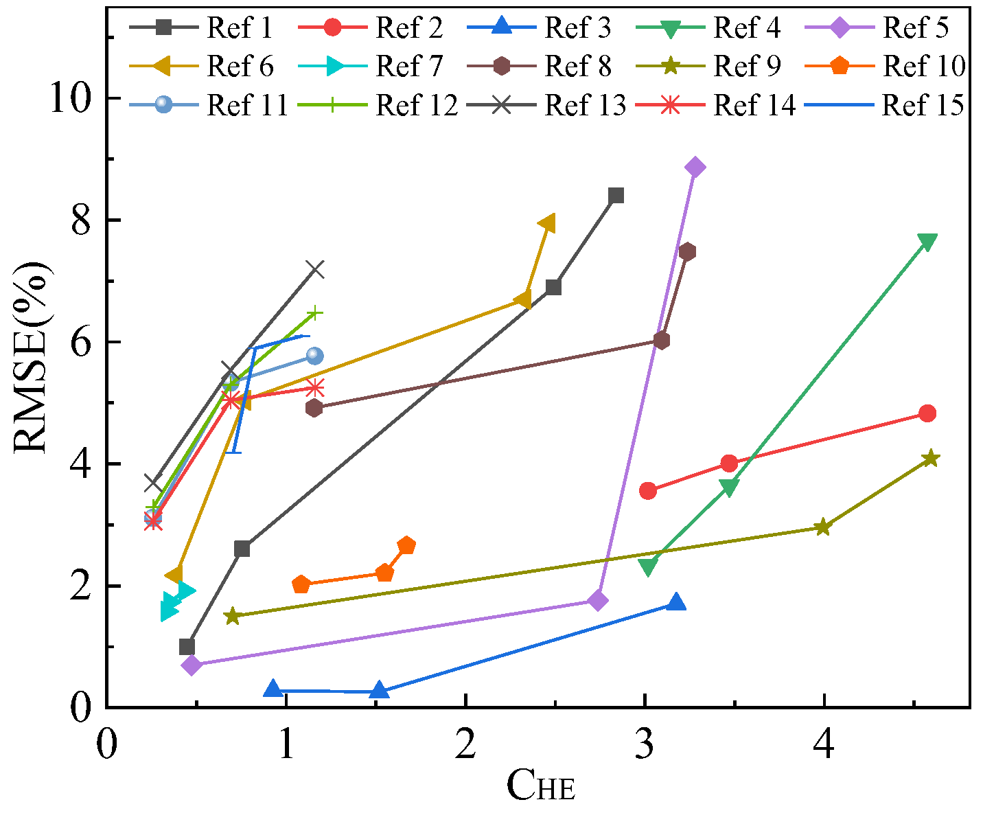
Figure 1. The root mean square error and its corresponding CHE value in the literature review. Ref 1 to Ref 15 in the figure refer sequentially to [4,6,11,14,17,20,28,32,33,34,35,36,37,38,39].
Applsci 15 04728 g001
Figure 2. Flow chart of the adaptive hybrid kernel method.
Applsci 15 04728 g002
Figure 3. Nonuniform discretization scheme used in the AGES.
Applsci 15 04728 g003
Figure 4. Flow chart of the adaptive grid evolution strategy.
Applsci 15 04728 g004
Figure 5. Flow chart of the AGES-AHK method and the full reconstruction process.
Applsci 15 04728 g005
Figure 6. 2D ROI configuration.
Applsci 15 04728 g006
Figure 7. The temperature contours of the three temperature phantoms under four coefHE values.
Applsci 15 04728 g007
Figure 8. Parametric investigation of the influence of the ε and RBF types on the reconstruction results. The red region represents the local zoom position.
Applsci 15 04728 g008
Figure 9. The reconstruction errors and the total calculation time of the three temperature phantoms.
Applsci 15 04728 g009
Figure 10. The temperature contour maps reconstructed by the finalized AGES-AHK method under four coefHE values.
Applsci 15 04728 g010
Figure 11. The reconstruct errors of three temperature phantoms under four coefHE values.
Applsci 15 04728 g011
Figure 12. The Cond(B) of three temperature phantoms under four coefHE values.
Applsci 15 04728 g012
Figure 13. The hotspot temperature error of three temperature phantoms under four coefHE values.
Applsci 15 04728 g013
Table 1. The CHE values of the three temperature phantoms under four coefHE values.
coefHECHE
Tfield1Tfield2Tfield3
0.13.262.232.34
0.26.515.224.08
0.516.5314.9615.28
132.0431.3334.02
Table 2. The reconstruction results of the AGES-AHK method.
CasecoefHEInput ValuesNRMSE/%Eh/%Dh/%
Tfield10.1fb = 0.3, κ = 1.5 × 10−40.601.190
0.2fb = 0.4, κ = 1.5 × 10−41.182.430
0.5fb = 0.2, κ = 1.5 × 10−42.901.390
1fb = 0.25, κ = 1 × 10−46.6119.010
Tfield20.1fb = 0.1, κ = 1.5 × 10−40.790.58, 0.741.41, 1.41
0.2fb = 0.2, κ = 1.5 × 10−43.062.28, 0.701.41, 1.41
0.5fb = 0.5, κ = 9 × 10−52.922.91, 4.180, 0
1fb = 0.4, κ = 7 × 10−53.8714.59, 13.490, 0
Tfield30.1fb = 0.8, κ = 1.5 × 10⁻⁴ 1.582.10, 0.86, 0.89 1.41, 3, 2
0.2fb = 0.4, κ = 7.5 × 10−52.184.08, 0.95, 0.55 1.41, 2.41, 1
0.5fb = 0.5, κ = 3 × 10−53.6514.94, 12.09, 8.202.24, 0, 1.41
1fb = 0.5, κ = 1 × 10−46.6724.98, 20.12, 22.961.41, 1, 0
Table 3. The hotspot position deviation of Tfield1.
coefHEDh/%
BasisAHKAGESAGES-AHK
0.10000
0.20000
0.50000
10000
Table 4. The hotspot position deviation of Tfield2.
coefHEDh/%
BasisAHKAGESAGES-AHK
0.11.41, 1.411.41, 1.410, 1.411.41, 1.41
0.20.14, 1.411.41, 1.411.41, 1.411.41, 1.41
0.50, 00, 00, 00, 0
10, 00, 00, 00, 0
Table 5. The hotspot position deviation of Tfield3.
coefHEDh/%
BasisAHKAGESAGES-AHK
0.11, 3.16, 6.321.41, 2, 3.161.41, 3, 31.41, 3, 2
0.23, 2.24, 3.161, 2.24, 21.41, 0, 31.41, 2.41, 1
0.52.24, 0, 22.24, 0, 2.241.41, 0, 12.24, 0, 1.41
12, 2, 1.411.41, 1.41, 12, 1, 11.41, 1, 0
Disclaimer/Publisher’s Note: The statements, opinions and data contained in all publications are solely those of the individual author(s) and contributor(s) and not of MDPI and/or the editor(s). MDPI and/or the editor(s) disclaim responsibility for any injury to people or property resulting from any ideas, methods, instructions or products referred to in the content.