Performance of Fine-Tuning Techniques for Multilabel Classification of Surface Defects in Reinforced Concrete Bridges

Abstract

Machine learning models often face challenges in bridge inspections, especially in handling complex surface features and overlapping defects that make accurate classification difficult. These challenges are common for image-based monitoring, which has become increasingly popular for inspecting and assessing the structural condition of reinforced concrete bridges with automated possibilities. Despite advances in defect detection using convolutional neural networks (CNNs), although challenges such as overlapping defects, complex surface textures, and data imbalance remain difficult, full fine-tuning of deep learning models helps them better adapt to these conditions by updating all the layers for domain-specific learning. The aim of this study is to demonstrate how effective the fine-tuning of several deep learning architectures for bridge damage classification allows for robust performance and the best utilization value of the methods. Six CNN architectures, ResNet-18, ResNet-50, ResNet-101, ResNeXt-50, ResNeXt-101 and EfficientNet-B3, were fine-tuned using the CODEBRIM dataset. Their performance was evaluated using Precision, Recall, F1 Score, Balanced Accuracy and AUC-ROC metrics to ensure a robust evaluation framework. This indicates that the EfficientNet-B3 and ResNeXt-101 models outperformed the other models and achieved the highest classification accuracy in all the error categories. EfficientNet-B3 showed the best-balanced Precision (0.935) and perfect Recall (1.000) in background classification, indicating its ability to distinguish defect-free areas from structural damage. These results highlight the potential of these models to improve automated bridge inspection systems and thus increase accuracy and efficiency in real-world applications, as well as provide guidance for the selection of methods based on whether accuracy or overall consistency is more important for a specific application.

1. Introduction

Traditional methods of damage detection in bridges are often time-consuming and require significant manual effort, despite the value they bring in terms of lifetime safety, performance and intervention measures for these structures [1]. Automated computer vision or image processing methods can often provide a more objective inspection while reducing uncertainties. Several methods exist in this regard, often with robotics involved. These methods are effective and can also positively influence the health and safety of workers but protect them from having to reach in far or into a potentially hazardous location. Machine learning techniques have become rapidly popular to improve robustness, efficiency, accuracy and Precision. However, such improvement is contingent upon real-life variabilities like variation illumination [2], environmental conditions [3], occlusion [2], motion blur [4] and turbidity for underwater conditions [5].

The availability of large and varied datasets and high processing power lead to high accuracy in image classification through deep learning (DL). Here, convolutional neural networks (CNNs) have the ability to extract features of defects from images to create meaningful representations for object recognition [6].

Computer vision algorithms for defect detection can be broadly categorized into four families: image classification, object detection, semantic segmentation and anomaly detection [7]. The present study focuses on deep learning-based classification due to its simplicity and suitability for scenarios where image-level annotation is available. Image processing of recent examples like San Francisco–Oakland Bay Bridge [8] and Morandi Bridge in Genoa, Italy [9], indicates cracks in components and failure of connections as critical causes of disasters where the classification of damages was very important and vital. Image classification is a fundamental task in visual recognition, encompassing object classification, detection and segmentation, with far reaching consequences in the safety and performance of bridge structures.

Traditional machine learning methods rely on manual feature design for image classification but often suffer from poor generalization and portability. CNNs address this limitation to a certain extent by extracting hierarchical features, pooling and dense layers, and architectures like AlexNet, VGGNet, GoogLeNet, ResNet, DenseNet, Xception, MobileNet, and EfficientNet have significantly advanced image classification accuracy and efficiency [10].

Recent developments in machine learning have extended beyond bridge inspection to include subsurface and tunnel-related structural assessments. For instance, Yang et al. [11] employed a probabilistic CNN–RF hybrid model to predict rock mass classification in TBM operations, while Yang et al. [12] proposed a feature fusion framework combining TBM operation data and cutter wear indicators. These studies reinforce the broader relevance of tuning strategies, data fusion and model interpretability across civil engineering domains.

Table 1. Some of the deep learning datasets and bridge databases.

Dataset Name	Total Images	Defect/Classes
ImageNet [13]	+15 M	Over 22,000 object classes
SDNET [14]	230 High-resolution (56,092 images for all classes)	Concrete cracks from bridges, walls, pavement
CODEBRIM [15]	1590 High-resolution (10,789 images for all classes)	Multi-label/Cracks, corrosion, spalling, etc.
SOFIA [16]	139,455 (53,805 are labeled)	Bridge components and structural defects
METU [17]	458 High-resolution (40,000 images for all classes)	Crack/No-crack
BCD [18]	6069	Bridge cracks/background
CDS [19]	1028	Surface damages in concrete bridges
ICCD [20]	1455	Cracks in bridges and towers
MCDS [21]	3607	Various concrete defects

presents an overview of some of the popular datasets and modern sources of images.

Table 2. Summary of CNN-based approaches for concrete defect detection, and classification accuracy values represent the highest reported result considering the best-performing model.

Author	Model	Pre-Trained on	Dataset	Defect Type	Accuracy
Dorafshan et al. [14]	AlexNet	IMAGENET	SDNET	Binary Crack	95.52%
Bhattacharya et al. [22]	Res2Net	-	CODEBRIM & SDNET	Multiple defects	92.70%
Su and Wang [23]	EfficientNetB0	IMAGENET	Li and Zhao & SDNET	Binary Crack	99.11%
Páques et al. [16]	DINO ViT/8	-	SOFIA	Multiple defects	89.20%
Mundt et al. [24]	Meta-learned	-	CODEBRIM	Multiple defects	72.19%
Rajadurai & Kang [25]	AlexNet	IMAGENET	Concrete Crack Images	Binary Crack	89.00%
Ali et al. [26]	Customized CNN	IMAGENET	SDNET, METU	Binary Crack	98.30%
Yang et al. [27]	VGG16	IMAGENET	METU, SDNET, BCD	Binary Crack	99.80%
Zhu et al. [28]	Inception-v3	IMAGENET	Self-collected	Multiple defects	97.80%
Zoubir et al. [29]	VGG16	IMAGENET	Self-collected	Multiple defects	97.10%
Bukhs et al. [30]	VGG16, Inception-v3, ResNet50	IMAGENET	CDS, SDNETv1, BCD, ICCD, MCDS, CODEBRIM	Multiple defects	90.00%

compares various CNN-based models, datasets and reported accuracies for both binary and multiple defects classification tasks in concrete structures.

This paper presents a framework to detect five types of bridge damage, including cracks, spalling, efflorescence, exposed bars and corrosion stains based on the ResNet-18/50/101, ResNeXt-50/101 and EfficientNet-B3 models. To boost the detection accuracy, a transfer learning method with fully pre-trained weights from the ImageNet dataset was used to improve the original models.

The model performance in concrete defect detection is highly dependent on fine-tuning strategies, especially in transfer learning scenarios. Full fine-tuning, partial tuning and parameter freezing are commonly used approaches. As shown in recent studies [26,27], tuning decisions not only influence accuracy but also significantly impact robustness across varying image contexts and data distributions. Understanding tuning is therefore not just about optimizing performance on a specific test set but about enabling models to generalize effectively unseen environments and defect types. The literature has already established that consistent and resilient features can be really important for various performance measures [31].

2. Materials and Methods

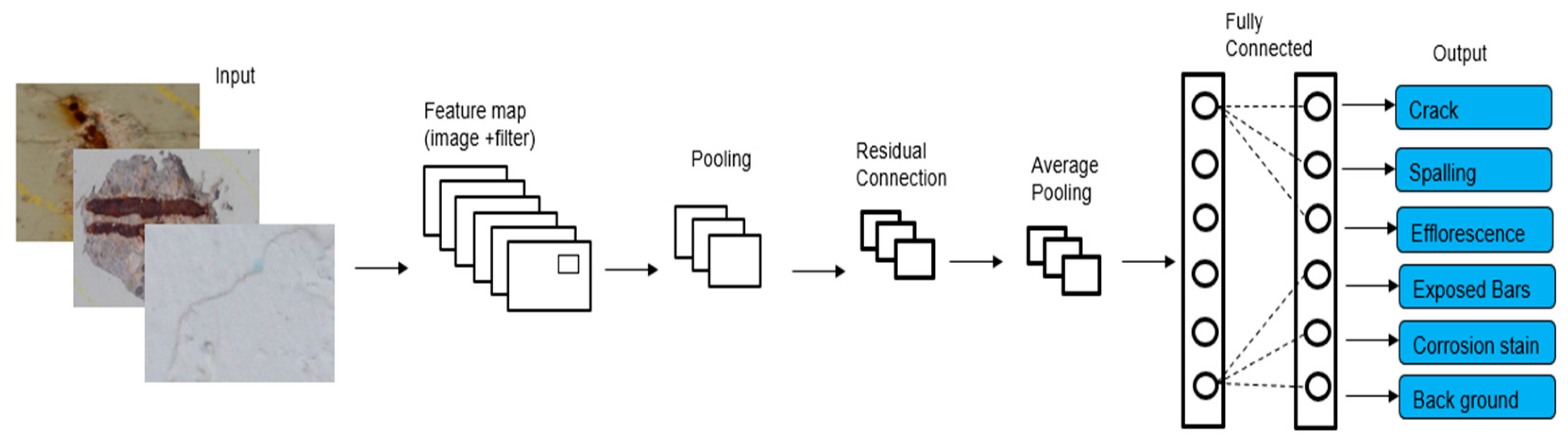
2.1. CNN Architecture

The following CNN architectures will be used:

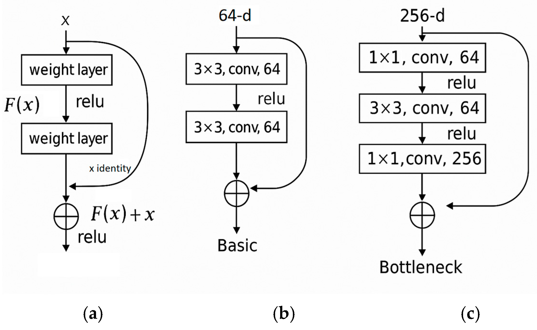
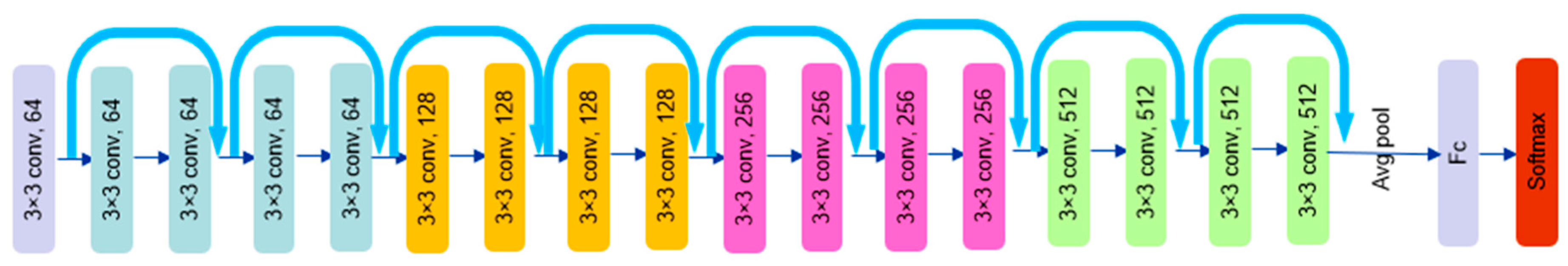
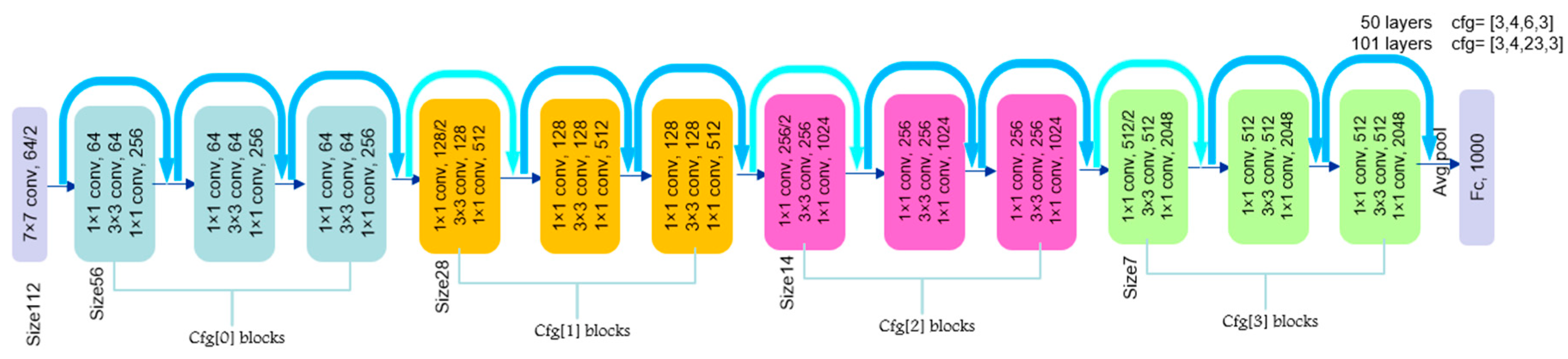
2.1.1. ResNet Network Architectures

In ResNet architecture, some inputs are passed directly to the next layers as opposed to the sequential layers in regular CNNs (Figure 1), allowing for deeper networks to be trained without the problem of vanishing points [32], resulting in an increase in model accuracy. As indicated in Figure 1a, the output F(x) is not transported to the next block until it is combined with x and put into ReLu activation function in the residual block [32]. Figure 1b shows one kind of residual block used in ResNet-18, and Figure 1c shows the other residual block used in ResNet-50/101. In this study, we choose the ResNet-18/50/101 model for the train and test sets, which architecture is shown in Figure 2 and Figure 3.

2.1.2. ResNeXt Network Architectures

ResNeXt is an extension of ResNet for improved performance using the concept of group convolution and cardinality [35], maintaining a simple structure while increasing the weight. Cardinality refers to the number of parallel paths in each convolutional block, which allows the network to learn more features without increasing the computational complexity. As shown in Figure 4a, ResNeXt uses 32 parallel paths, each containing a combination of convolutional layers. This design allows the network to process more data in parallel.

An advantage of ResNeXt is the simplicity in the design. While ResNet uses direct connections to create shorter paths, ResNeXt provides better generalization by adding parallel groups (Figure 4b) allowing for the same final output with less parameters via early concatenation. This approach of utilizing parallel groups is called grouped convolution. Figure 4c shows a 3 × 3 convolutional layer divided into 32 groups, leading to the requirement of less memory and reducing computations through the reduction of connections between the input and output, compromising the model accuracy.

Table 3. Architectural comparison of ResNet and ResNeXt variants in terms of depth, width and computational cost [32,35]. # Params = number of parameters; FLOPs = number of floating-point operations.

Stage	Output	ResNet-18	ResNet-50	ResNet-101	ResNeXt-50	ResNeXt-101
conv1	112 × 112	7 × 7, 64, stride 2	7 × 7, 64, stride 2	7 × 7, 64, stride 2	7 × 7, 64, stride 2	7 × 7, 64, stride 2
conv2	56 × 56	3 × 3 max pool, stride 2	3 × 3 max pool, stride 2	3 × 3 max pool, stride 2	3 × 3 max pool, stride 2	3 × 3 max pool, stride 2
		[3 × 3, 64] × 2	$\left[\begin{array}{c}1\times 1,64\\ 3\times 3,64\\ 1\times 1,256\end{array}\right]$ × 3	$\left[\begin{array}{c}1\times 1,64\\ 3\times 3,64\\ 1\times 1,256\end{array}\right]$ × 3	$\left[\begin{array}{c}1\times 1,128\\ 3\times 3,128\\ 1\times 1,256\end{array}\right]$ × 3, C = 32	$\left[\begin{array}{c}1\times 1,128\\ 3\times 3,128\\ 1\times 1,256\end{array}\right]$ × 3, C = 32
conv3	28 × 28	[3 × 3, 128] × 2	$\left[\begin{array}{c}1\times 1,128\\ 3\times 3,128\\ 1\times 1,512\end{array}\right]$ × 4	$\left[\begin{array}{c}1\times 1,128\\ 3\times 3,128\\ 1\times 1,512\end{array}\right]$ × 4	$\left[\begin{array}{c}1\times 1,256\\ 3\times 3,256\\ 1\times 1,512\end{array}\right]$ × 4, C = 32	$\left[\begin{array}{c}1\times 1,256\\ 3\times 3,256\\ 1\times 1,512\end{array}\right]$ × 4, C = 32
conv4	14 × 14	[3 × 3, 256] × 2	$\left[\begin{array}{c}1\times 1,256\\ 3\times 3,256\\ 1\times 1,1024\end{array}\right]$ × 6	$\left[\begin{array}{c}1\times 1,256\\ 3\times 3,256\\ 1\times 1,1024\end{array}\right]$ × 23	$\left[\begin{array}{c}1\times 1,512\\ 3\times 3,512\\ 1\times 1,1024\end{array}\right]$ × 6, C = 32	$\left[\begin{array}{c}1\times 1,512\\ 3\times 3,512\\ 1\times 1,1024\end{array}\right]$ × 23, C = 32
conv5	7 × 7	[3 × 3, 512] × 2	$\left[\begin{array}{c}1\times 1,512\\ 3\times 3,512\\ 1\times 1,2048\end{array}\right]$ × 3	$\left[\begin{array}{c}1\times 1,512\\ 3\times 3,512\\ 1\times 1,2048\end{array}\right]$ × 3	$\left[\begin{array}{c}1\times 1,1024\\ 3\times 3,1024\\ 1\times 1,2048\end{array}\right]$ × 3, C = 32	$\left[\begin{array}{c}1\times 1,1024\\ 3\times 3,1024\\ 1\times 1,2048\end{array}\right]$ × 3, C = 32
fc	1 × 1	Global average pool 1000-d fc, softmax	Global average pool 1000-d fc, softmax	Global average pool 1000-d fc, softmax	Global average pool 1000-d fc, softmax	Global average pool 1000-d fc, softmax
# Params		11.7 × 106	25.5 × 106	44.5 × 106	25.0 × 106	44.2 × 106
FLOPs		1.8 × 109	4.1 × 109	7.6 × 109	4.2 × 109	8.0 × 109

presents a comparative overview of the architectures of the ResNet and ResNeXt models, including ResNet-18, ResNet-50, ResNet-101 and their ResNeXt counterparts. While ResNet-18 uses basic 3 × 3 convolution blocks, the deeper ResNet-50 and ResNet-101 models employ bottleneck blocks (1 × 1 → 3 × 3 → 1 × 1). ResNeXt-50 and ResNeXt-101 follow the same bottleneck design but introduce grouped convolutions with a cardinality of 32, allowing the model to learn richer features with minimal increase in the parameters and computation. The main difference between the “50” and “101” variants lie in the number of residual blocks, especially in stage 4 (conv4). ResNeXt-101, being the deepest, offers the most expressive power.

2.1.3. EfficientNet-B3 Network Architectures

The EfficientNet-B3 architecture is shown in Figure 5, which starts with a 300 × 300 × 3 input image and extracts image features by passing through multiple convolutional and (Mobile Inverted Bottleneck Convolution) MBConv layers, which allows for improved computational efficiency. First, a 3 × 3 convolutional layer is applied to obtain the initial features. Then, several MBConv blocks, more optimized than the residual blocks in ResNet, are used for image processing. Unlike conventional residual blocks that connect from a low-dimensional path to a high-dimensional path, MBConv first expands the features, then processes them and finally reduces the features to the original dimensions. ResNet uses conventional residual connections that keep the original information value directly connected to the output layer. MBConv uses Inverted Residual Connections that expand, process and then do it again. These blocks are applied in multiple stages with 3 × 3 and 5 × 5 kernels, reducing the feature dimension and increasing the number of filters. Finally, a 1 × 1 convolution layer, a pooling stage and a fully connected (FC) layer produce the final feature vector and send it to a classifier.

Unlike ResNet, which only increases the depth of the network, EfficientNet performs simultaneous optimization on the depth, width and resolution of the image, which leads to higher accuracy with fewer calculations. This makes EfficientNet-B3 computationally lighter and faster and offers better accuracy in computer vision tasks. In fact, the EfficientNet model provides better accuracy and improves efficiency by reducing the parameters and FLOPS (floating-point operations per second) manifold [36].

2.2. Fine-Tuning and Transfer Learning Strategies

The chosen models, ResNet, ResNeXt and EfficientNet, are three diverse architectural design philosophies in deep convolutional neural networks. ResNet models are essentially residual connections to help with the learning of deep features. ResNeXt, with the introduction of grouped convolutions, allows the model to process on multiple parallel paths of information that may improve the detection of fine-grained features or overlapping defect patterns. EfficientNet-B3 employs a compound scaling approach that uniformly scales the depth, width and resolution of the network, allowing it to better capture fine texture variations and small-scale surface defect features.

Real-life situations often come with imperfect and limited data with complex information and related features of interest. Transfer learning and fine-tuning are critically important for improving the efficiency and speed of CNN training; typically, pre-trained models are loaded on large datasets (e.g., ImageNet), and the final layers of the model are then modified accordingly.

First, the weights of all the convolutional layers of the ResNet, ResNeXt and EfficientNet models are initialized using pre-trained weights from the ImageNet dataset [13]. These pre-trained convolutional layers act as powerful feature extractors for images [37]. In this study, we apply a full fine-tuning approach, meaning that all layers of the network, including the convolutional ones, are updated during training. This differs from the standard transfer learning strategy, which typically involves freezing the convolutional base and re-training only the fully connected (FC) layers [38,39]. Fine-tuning all the layers allows the model to better adapt to the domain-specific characteristics of concrete defect images [27].

Figure 6 illustrates the key differences between conventional transfer learning and the full fine-tuning approach employed in this study. While transfer learning typically updates only the final classification layers, full fine-tuning involves training the entire network, including all convolutional and fully connected layers. This strategy enables the model to adapt more effectively to the specific patterns and features present in the target domain.

By keeping all of the model, including the convolutional layers, trainable, this method enables a model to adjust to a new classification job. Because residual blocks are used in the architecture of the ResNet-18/50/101 models, the network can train deep layers without experiencing a gradient collapse. Due to cardinality, ResNeXt-50/101 expands on this approach and enhances the model performance without adding complexity. In contrast, EfficientNet-B3 employs an efficient scaling technique to expand the network’s size, reducing computational resource usage while preserving accuracy. Depending on the computing requirements and data complexity, these architectural variations will demonstrate varied performances.

The backbone architectures of all the CNN models (ResNet, ResNeXt and EfficientNet-B3) remain unchanged. However, to support multi-label classification, we replaced the original classification head of each model with a custom fully connected output layer consisting of six units, each corresponding to one defect class. A sigmoid activation function was applied to allow independent probability outputs. This new output layer was placed on top of the global average pooling layer. The rest of the network was kept structurally intact, but all the layers were fine-tuned during training.

In order to detect bridge damage and enhance the classification accuracy, the improved models (ResNet-18/50/101, ResNeXt-50/101 and EfficientNet-B3) were then trained end to end (from input to output) on a collection of more than 10,000 photos that contained both test and training data. Measures like Balanced Accuracy, Recall, and F1-Score were used to assess which architecture yielded the best results. It should be noted that the study performed a comparative evaluation of full fine-tuning strategies using well-known architectures on a multi-label surface defect dataset. By applying consistent training conditions across all the models, the study aims to reveal performance trade-offs and practical deployment insights for bridge inspection tasks.

3. Dataset

The CODEBRIM [15] dataset was developed to address the need for a more diverse collection of structural defects that frequently overlap in real-world scenarios. In practical inspections, visual defects such as cracks, corrosion and surface deterioration are influenced by multiple factors, including lighting conditions, varying angles of image capture and diverse surface characteristics. Therefore, applying DL in this domain necessitates sampling from real-world contexts to ensure that models can deliver accurate and reliable performance in complex, real-life conditions.

CODEBRIM [15] includes images from 30 different bridges, each exhibiting various levels of deterioration and structural damage. The CODEBRIM dataset includes images collected under diverse environmental and structural conditions, reflected in variations in lighting, surface textures and types of visible defects. This diversity suggests coverage of a broad range of real-world bridge settings, supporting the generalizability of the trained models in different environments.

The dataset covers five common types of defects: cracks, spalling, exposed reinforcement bars, efflorescence and corrosion. Cracks are often critical defects in concrete bridges, as they can lead to reduced structural integrity, decreased durability, increased safety risks, higher maintenance costs and functional degradation [40]. Spalling or delamination can cause a reduction in structural strength and increase in maintenance and repair costs. Severe weather conditions such as acid rain, freeze–thaw cycles and temperature changes can erode concrete, exposing the reinforcement bars. Heavy traffic and constant mechanical wear can erode the concrete surface as well.

Corrosion, a critical issue in reinforced concrete structures, arises from the electrochemical breakdown of the reinforcement. Efflorescence in concrete bridges is a common phenomenon and can be indicative of underlying moisture issues. Materials used in concrete bridges, such as cement, aggregates and water, can contain soluble salts. These salts become mobile when in contact with water. Bridges in regions with high humidity, heavy rainfall or near bodies of water are more prone to efflorescence.

Overlapping of defects: Concrete defects are intimately linked. The expansion of reinforcement corrosion causes tensile stresses in the concrete, which can lead to cracking and spalling. Exposed bars can be a consequence of spalling. Amirkhani et al. [41] found that exposed bars and spalling defects occurred together more than 70% of the time. Figure 7 illustrates some examples of the single and overlapping of defects.

The classification task is formulated as a multi-label, where each image can be associated with one or more defect types. The five annotated defect categories in the CODEBRIM dataset are defined as follows:

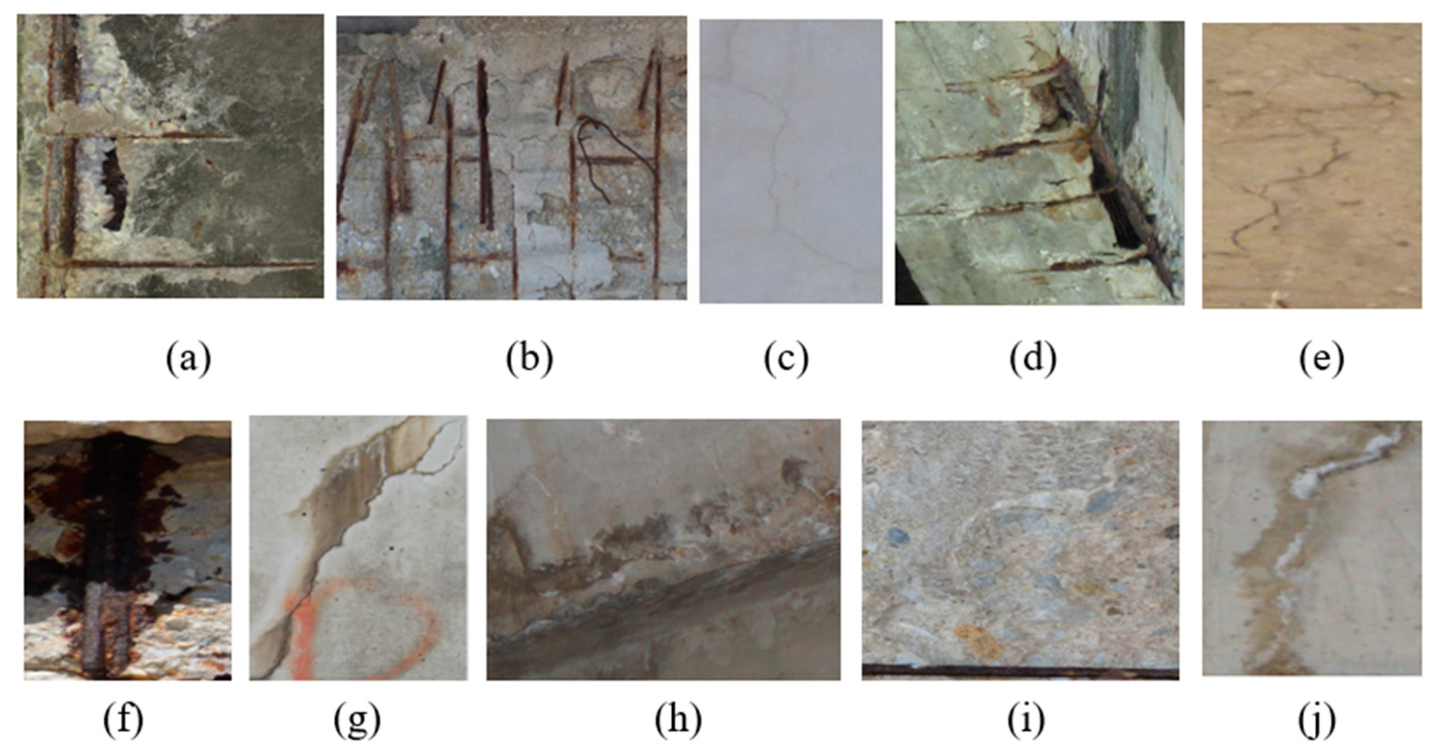
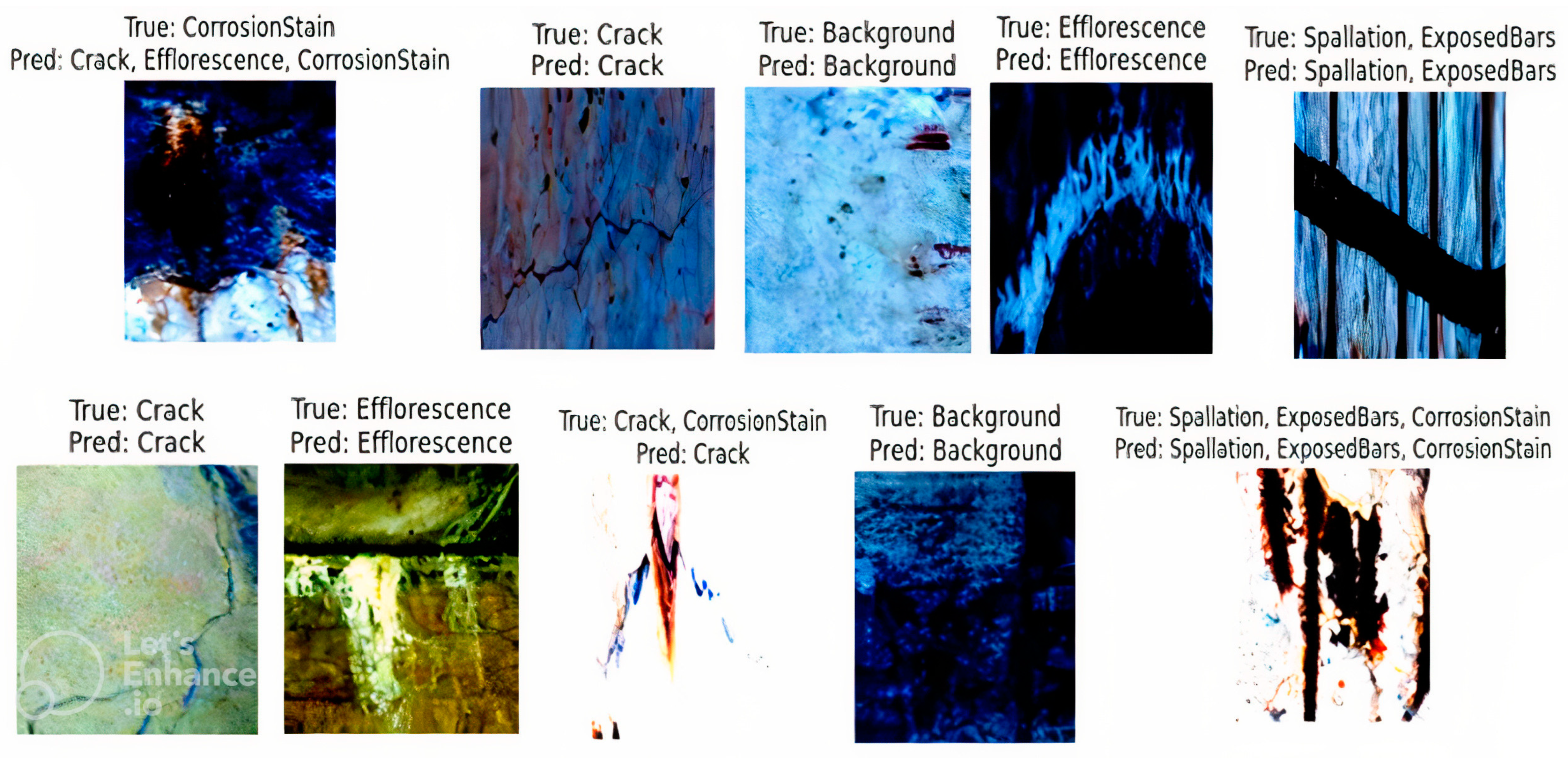
• Crack—visible linear fracture or separation in the concrete surface. Although cracks may exhibit various typologies such as hairline, vertical or diagonal cracks, the CODEBRIM dataset annotates all crack types under a single “crack” label. Consequently, our classification model is trained to recognize cracks as a general category.
• Spalling—surface flaking or detachment of concrete material.
• Efflorescence—white crystalline deposits resulting from salt leaching.
• Corrosion stain—discoloration due to rust formation, often near steel reinforcements.
• Exposed bars—visible steel reinforcement due to severe concrete loss.

These classes are not mutually exclusive and may cooccur in the same image.

The CODEBRIM dataset supports multi-label annotations, where multiple defects such as cracks, corrosion and exposed bars may cooccur in a single image. While the dataset does not define composite classes explicitly, such overlaps are represented through simultaneous binary labels. Our model uses sigmoid activation to allow the independent prediction of each defect, enabling robust detection even in overlapping scenarios (e.g., a spalled area with exposed reinforcement and corrosion stains).

Bridges that were free of defects were excluded from the analysis, allowing the dataset to focus solely on damaged and challenging structures. The CODEBRIM dataset provides defect images captured under diverse environmental conditions and from multiple views and scales, although specific details regarding camera configurations or bridge selection criteria are not provided explicitly [15].

Table 4. Number of classes counts in this study.

Class	Train Dataset	Validation Dataset	Test Dataset	Sum
Crack	2208	149	150	2507
Spalling	1608	140	150	1898
Efflorescence	543	140	150	833
Exposed Bars	1215	142	150	1507
Corrosion Stain	1263	146	150	1559
Background	2185	150	150	2485
Sum	9022	867	900	10,789

shows the class counts in the train, test and validation datasets in this study.

Based on the stated database, Figure 7 shows part of the methodological architecture used in this study.

Figure 8 illustrates the architecture of the ResNet-based model employed in this study for the multi-label classification of concrete bridge defects. The input images, sourced from the CODEBRIM dataset, are first passed through multiple convolutional layers, where feature maps are generated by applying learned filters. These maps are then downsampled via pooling layers, and residual connections are introduced to facilitate deep feature learning and mitigate the vanishing gradient problem. Following this, global average pooling is applied to condense spatial information, and the resulting features are fed into fully connected layers.

The final output consists of multi-label predictions (crack, spalling, efflorescence, exposed bars, corrosion stains and background), with a sigmoid activation applied to each output node to enable independent probabilities for cooccurring defect classes.

4. Discussion

4.1. Training Results

This paper compares pre-trained CNN classifiers ResNet-18/50/101, ResNeXt-50/101 and EfficientNet-B3 for the CODEBRIM database, following full fine-tuning and using the same number of epochs (25), and the batch size was 32. All models were compiled with the loss function Focal Loss, a variant of BCEWithLogitsLoss, to improve the performance on imbalanced or hard-to-classify examples, where a model may predict dominant examples (classes with a lot of data) and ignore rarer examples. This approach is particularly effective in imbalanced datasets, such as defect classification tasks, and was originally proposed by Lin et al. [42].

The dataset was split into training, validation and test sets based on class-balanced partitioning. The class distribution across the subsets is presented in Table 4. For preprocessing, input images were resized to 224 × 224 for ResNet and ResNeXt and 300 × 300 for EfficientNet-B3 and normalized using ImageNet statistics. Data augmentation (random horizontal flip and rotation) was applied only to the training set. In this study, we applied standard augmentations, including horizontal flipping and random rotation, to increase the dataset diversity. These simple yet effective transformations were selected due to their relevance to typical variations in bridge inspection imagery.

The same preprocessing pipeline was applied across all models to ensure comparability. The use of consistent data loaders and identical training parameters across all models ensures fair benchmarking and supports the reproducibility of the results. All parameters in the classifiers were optimized with the AdamW optimizer with an initial learning rate of 0.001.

Figure 9a shows a steady improvement across all models over all epochs; the ResNet-18 model has the lowest accuracy (86.1%) at the beginning of training, while more sophisticated models such as ResNeXt-50 and EfficientNet-B3 start with accuracies of 89.71% and 89.02%. For EfficientNet-B3 and ResNeXt-101 at the end of the training, their accuracies reached 97.57% and 98.46%. They were consistently among the models with the highest accuracy. It shows these models have the ability to learn better and extract deeper features. ResNet-50 and ResNet-101 also performed well, achieving accuracies of 97.39% and 97.7%, but were still slightly lower than EfficientNet-B3 and ResNeXt-101. In contrast, ResNet-18 had the lowest accuracy at 95.55%, indicating the model’s limitations in learning more complex features of the data.

Figure 9b demonstrates that all the models successfully minimize errors as the training progresses. At the beginning of training, the ResNet-18 model has the highest error rate with a value of 0.0871, while the ResNet-50, ResNet-101, ResNeXt-50, ResNeXt-101 and EfficientNet-B3 models have lower error rates and perform better in optimization from the beginning. As the most optimal models, EfficientNet-B3 and ResNeXt-101 record the lowest error rate at the end of the training, which indicates their high ability to learn complex data features. In contrast, ResNet-18 has a slower error rate, and its loss rate remains at 0.0303 at the end of training, which is still higher than the other models. ResNet-50 and ResNet-101 perform moderately well.

4.2. Evaluation Metrics

Several evaluation factors were used for quantifying the classification tasks [43]. Precision (Equation (1)) determines what percentage of the examples that the model predicted as a particular class actually belong to that class.

$$\mathrm{Precision}={\displaystyle \frac{\mathrm{T}\mathrm{P}}{\mathrm{T}\mathrm{P}+\mathrm{F}\mathrm{P}}}$$

(1)

where TP (True Positive) is the number of cases that the model correctly identified as that class, FP (False Positive) is the number of cases that the model incorrectly identified as that class, Recall (Equation (2)) determines what percentage of the total number of true examples of a class the model correctly identified and FN (False Negative) is the number of cases that the model incorrectly identified as another class.

$$\mathrm{Recall}={\displaystyle \frac{\mathrm{T}\mathrm{P}}{\mathrm{T}\mathrm{P}+\mathrm{F}\mathrm{N}}}$$

(2)

F1-Score harmonic the means of Precision and Recall (Equation (3)), so that, when one of these two values is low, the F1-Score also goes down.

$$\mathrm{F}1\text{-}\mathrm{Score}=2\times {\displaystyle \frac{\mathrm{P}\mathrm{r}\mathrm{e}\mathrm{c}\mathrm{i}\mathrm{s}\mathrm{i}\mathrm{o}\mathrm{n}+\mathrm{R}\mathrm{e}\mathrm{c}\mathrm{a}\mathrm{l}\mathrm{l}}{\mathrm{P}\mathrm{r}\mathrm{e}\mathrm{c}\mathrm{i}\mathrm{s}\mathrm{i}\mathrm{o}\mathrm{n}\times \mathrm{R}\mathrm{e}\mathrm{c}\mathrm{a}\mathrm{l}\mathrm{l}}}$$

(3)

The Balanced Accuracy (BA) metric is better than simple accuracy when the data are unbalanced, measuring the average of Sensitivity and Specificity (Equation (4))

$$\mathrm{BA}={\displaystyle \frac{\mathrm{S}\mathrm{e}\mathrm{n}\mathrm{s}\mathrm{i}\mathrm{t}\mathrm{i}\mathrm{v}\mathrm{i}\mathrm{t}\mathrm{y}+\mathrm{S}\mathrm{p}\mathrm{e}\mathrm{c}\mathrm{i}\mathrm{f}\mathrm{i}\mathrm{c}\mathrm{i}\mathrm{t}\mathrm{y}}{2}}$$

(4)

where Sensitivity is defined the same as Recall, while Specificity is the rate of correct identification of negative samples (Equation (5)):

$$\mathrm{Specificity}={\displaystyle \frac{\mathrm{T}\mathrm{N}}{\mathrm{T}\mathrm{N}+\mathrm{F}\mathrm{P}}}$$

(5)

TN (True Negative) is the number of negative classes predicted to be negative classes [43].

Table 5. Model evaluation index of ResNet-18/50/101.

Class	ResNet-18				ResNet-50				ResNet-101
	Precision	Recall	F1-Score	Balanced Accuracy	Precision	Recall	F1-Score	Balanced Accuracy	Precision	Recall	F1-Score	Balanced Accuracy
Crack	0.760	0.907	0.827	0.909	0.777	0.927	0.845	0.922	0.803	0.927	0.861	0.928
Spalling	0.703	0.867	0.776	0.876	0.742	0.900	0.813	0.901	0.734	0.900	0.808	0.899
Efflorescence	0.849	0.832	0.841	0.893	0.894	0.846	0.869	0.907	0.909	0.872	0.890	0.923
Exposed Bars	0.897	0.933	0.915	0.950	0.965	0.913	0.938	0.951	0.946	0.933	0.940	0.958
Corrosion Stain	0.652	0.913	0.761	0.881	0.739	0.927	0.822	0.913	0.730	0.920	0.814	0.907
Background	0.865	0.940	0.901	0.947	0.898	0.940	0.919	0.953	0.918	0.973	0.945	0.973
Overall	0.778	0.899	0.834	0.909	0.826	0.909	0.865	0.925	0.831	0.921	0.874	0.931

and

Table 6. Model evaluation index of ResNeXt-50/101 and EfficientNet-B3.

Class	ResNeXt-50				ResNeXt-101			EfficientNet-B3
	Precision	Recall	F1-Score	Balanced Accuracy	Precision	Recall	F1-Score	Balanced Accuracy	Precision	Recall	F1-Score	Balanced Accuracy
Crack	0.825	0.940	0.879	0.939	0.838	0.933	0.883	0.939	0.816	0.947	0.877	0.940
Spalling	0.756	0.907	0.824	0.908	0.771	0.900	0.831	0.909	0.729	0.913	0.811	0.904
Efflorescence	0.903	0.879	0.891	0.925	0.956	0.872	0.912	0.930	0.912	0.832	0.870	0.904
Exposed Bars	0.966	0.933	0.949	0.961	0.938	0.913	0.926	0.947	0.926	0.913	0.919	0.945
Corrosion Stain	0.758	0.920	0.831	0.914	0.765	0.913	0.833	0.913	0.828	0.933	0.878	0.937
Background	0.918	0.967	0.942	0.970	0.901	0.973	0.936	0.970	0.893	1.000	0.943	0.981
Overall	0.847	0.924	0.884	0.936	0.855	0.918	0.885	0.935	0.844	0.923	0.882	0.935

compare the performance of six different models for concrete damage classification using the CODEBRIM dataset. Four metrics are used to evaluate the ResNet (18, 50 and 101); ResNeXt (50 and 101) and EfficientNet-B3 models: Precision, Recall, Balanced Accuracy and F1-Score. These models’ architecture and complexity differ, causing them to perform better in some classes and worse in others.

Among the ResNet models, ResNet-18 demonstrates the weakest performance, with lower F1-Scores and Balanced Accuracy across all defect classes. This is particularly evident in the “corrosion stain” category, where its F1-Score is only 0.761, suggesting difficulties in correctly distinguishing this defect from others. ResNet-50 improves upon ResNet-18 in all the metrics, especially in detecting “crack” and “spalling”, where their F1-Scores reach 0.845 and 0.813, respectively. ResNet-101 further enhances the classification performance, achieving the highest scores within the ResNet family, particularly in identifying “efflorescence” and “exposed bars”, where its F1-Scores surpass 0.89.

ResNeXt-50 and ResNeXt-101, which utilize grouped convolutions for better feature extraction, outperform their ResNet counterparts. ResNeXt-50 surpasses ResNet-50 in nearly all the categories, with a notable improvement in “crack” (F1-Score of 0.879) and “spalling” (F1-Score of 0.824). ResNeXt-101 further refines this performance, providing an overall Balanced Accuracy of 0.935 and particularly excelling in “efflorescence” and “corrosion stain”, where its F1-Scores exceed those of ResNet-101. The improvements in the ResNeXt models suggest that adopting grouped convolutions enhances feature representation and helps in better distinguishing similar structural defects.

EfficientNet-B3 emerges as the best-performing model among all the tested architectures. It demonstrates superior Recall in detecting “crack” (0.947), meaning it successfully identifies nearly all instances of this defect. Moreover, in the “corrosion stain” category, EfficientNet-B3 achieves the highest F1-Score of 0.878, highlighting its effectiveness in handling difficult-to-distinguish defects. In the “background” class, this model records the highest Recall (1.000) and F1-Score (0.943), showcasing its Precision in correctly classifying defect-free areas. Compared to ResNeXt-101, EfficientNet-B3 slightly underperforms in a few categories, such as “efflorescence”, but maintains the best overall performance with a Balanced Accuracy of 0.935 and an overall F1-Score of 0.882.

The performance differences among the six models can be explained through their architectural depth, parameter count and how these factors interact with the full fine-tuning process. ResNet-18, being the shallowest with around 11 M parameters, offers fast convergence and decent generalization under limited data, but its limited depth may hinder the learning of complex defect features. ResNet-50 and ResNet-101 progressively increase in depth (with ~23 M and ~45 M parameters, respectively), allowing for more detailed feature extraction but also introducing a higher risk of overfitting. ResNeXt-50 and ResNeXt-101 introduce grouped convolutions (cardinality), which expand feature diversity without significantly increasing the parameters, making them efficient for capturing subtle defect variations. EfficientNet-B3, with compound scaling of the width, depth and resolution, achieves strong performance due to its balanced design, though it is more sensitive to hyperparameter tuning and training dynamics. Under full fine-tuning, where all layers are updated, these structural differences play a more prominent role, as the model’s ability to adapt feature hierarchies becomes crucial for multi-label defect recognition.

CNN-based models on the CODEBRIM dataset. Models from previous studies, including MetaQNN [24], VGG16, Inception-V3 and ResNet-50 [30], have reported accuracies ranging from 72.19% to 90.00%. In contrast, the models implemented in this study, ResNet-18, ResNet-50, ResNet-101, ResNeXt-50, ResNeXt-101 and EfficientNet-B3, consistently outperformed earlier methods, achieving accuracies from 90.90% to 93.60%.

This performance gain can be attributed not only to the use of deeper and more advanced network architectures but also to the application of full fine-tuning, which allowed the models to better adapt to the dataset-specific features. Moreover, the use of the focal loss function, which emphasizes harder and minority class examples during training, contributed to improved classification performance, especially in cases of class imbalance. Among them all, ResNeXt-50 achieved the highest accuracy (93.60%), followed closely by EfficientNet-B3 and ResNeXt-101 (both at 93.50%).

Table 7. Comparative study of model accuracies using CODEBRIM data.

Model	MetaQNN [24]	VGG16 [30]	Inception-V3 [30]	ResNet-50 [30]	Resnet-18 This Study
Accuracy%	72.19%	88.00%	89.00%	90.00%	90.90%
Model	Resnet-50 This study	Resnet-101 This study	ResNeXt-50 This study	ResNeXt-101 This study	Efficient-B3 This study
Accuracy%	92.50%	93.10%	93.60%	93.50%	93.50%

shows that modern architectures can significantly outperform traditional models in multi-label bridge defect classification. This highlights the importance of architectural choice and tuning strategies in real-world infrastructure monitoring systems.

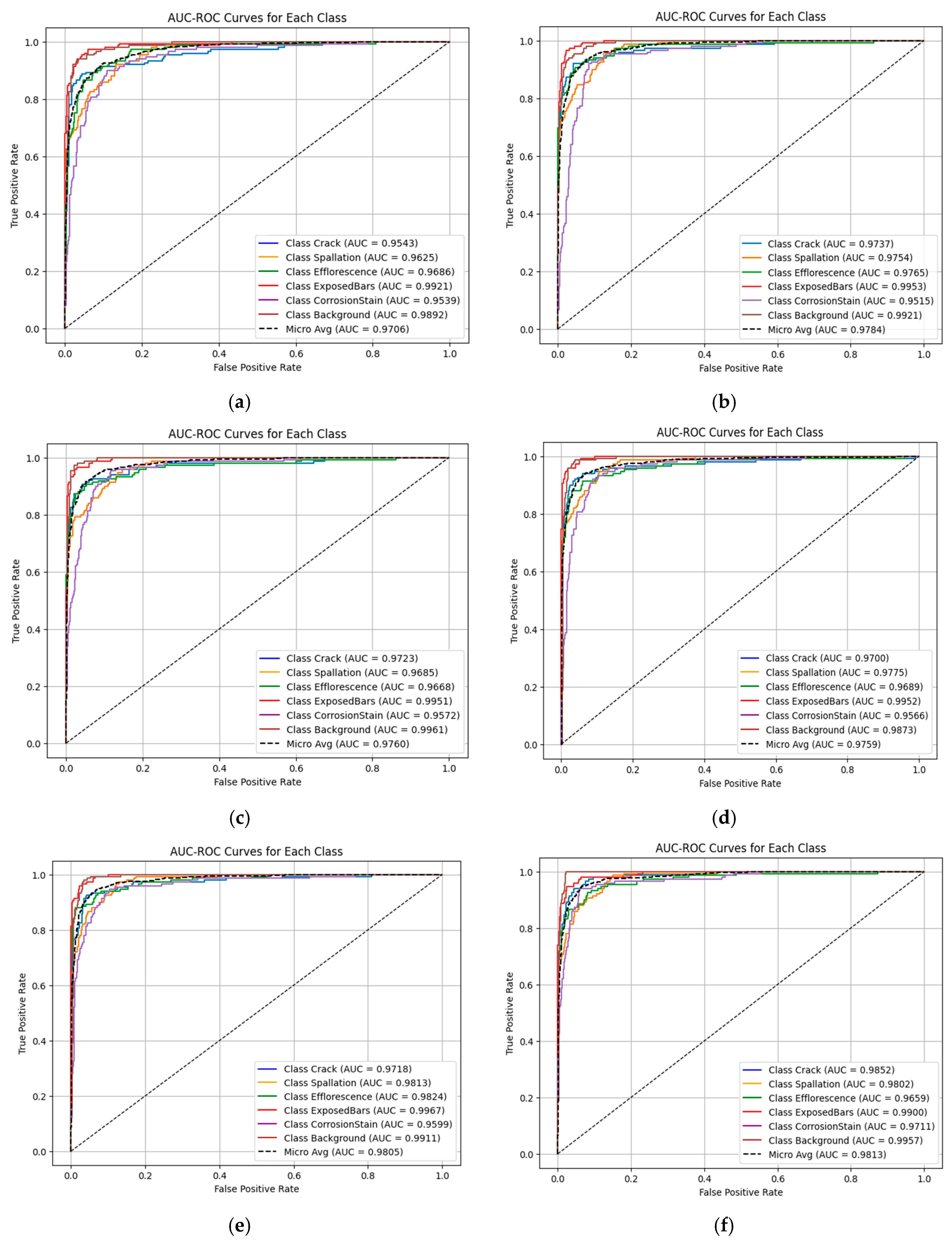
4.3. AUC-ROC Analysis

This study used the AUC-ROC (area under the receiver operating characteristic curve) metric to evaluate and compare deep learning models, because in the unbalanced class database, accuracy alone cannot indicate the true performance of the model, as a model that predicts the dominant class may have high accuracy but poor performance in identifying rare classes. This metric is one of the most useful for evaluating classification model performance, especially when class distributions are uneven. AUC-ROC computes the area under the ROC curve for all possible choice criteria and transforms it into a single integer. This score shows the model’s overall ability to distinguish between positive and negative data, regardless of a specific threshold. The AUC-ROC values range from 0 to 1, with values around 1 indicating excellent model performance and values of 0.5 or lower indicating poor random performance.

In addition to the AUC-ROC, the Precision, Recall, F1-Score and Balanced Accuracy metrics are provided to round out the model evaluation (Table 5 and Table 6). Since this study was conducted on the CODEBRIM dataset, which involves multi-class and multi-label classification, it is important to state the difference between standard AUC and micro-average AUC (Mic Avg AUC). Per-class AUC measures the area under the ROC curve for each class separately. This value indicates how well the model is able to detect a particular defect. Instead of calculating it separately for each class, micro-average AUC (Mic Avg AUC) calculates the sum of the TP, FP, TN and FN across all classes and then obtains the AUC value. This method is more efficient in situations where there are unbalanced data. Considering that our data contain defects with an unbalanced distribution, Mic Avg AUC is a more appropriate index to evaluate the overall ability of models to detect real defects in real-world conditions.

Figure 10 presents the ROC curves for multiple deep learning models, illustrating their classification performance. The x-axis represents the False Positive Rate (FPR), while the y-axis denotes the True Positive Rate (TPR). Among the tested architectures, the ResNet models (ResNet-18, ResNet-50 and ResNet-101) exhibit strong classification performance, but their effectiveness varies across defect types. For instance, the “exposed bars” class consistently achieves a high AUC, close to 1, across all the models. However, classes like “corrosion stain” and “spalling” show relatively lower AUC values in some ResNet variants, indicating that these models struggle to differentiate them from similar defect patterns.

The ResNeXt series (ResNeXt-50 and ResNeXt-101) shows improvements over ResNet, primarily due to grouped convolutions, which enhance feature extraction and representation. ResNeXt-101, in particular, achieves an AUC above 0.96 for most classes and even reaches 0.99 for certain defect types, demonstrating superior classification accuracy. Among all the models, EfficientNet-B3 emerges as the best-performing architecture. Its AUC remains above 0.96 across all classes, and for some categories, it reaches a close score of 1. This suggests that EfficientNet-B3 is highly effective in distinguishing structural defects, providing a robust decision boundary while maintaining computational efficiency compared to deeper ResNet and ResNeXt models. Ultimately, ResNeXt-101 and EfficientNet-B3 stand out as the top performers, with EfficientNet-B3 achieving the most reliable predictions across all the defect classes.

Figure 11 shows examples of the model predictions compared to the actual values. In some cases, the model correctly identified the defect class, such as crack and efflorescence. However, in some more complex examples, the model only identified one of the defect classes and ignored the other part. Also, the background was correctly identified, which shows that the model is able to distinguish between the defect and the background. There were some examples of a completely successful prediction, where all defect classes were correctly identified. These results indicate that the model performs well in most cases, but they show that detecting mixed defects can be challenging.

From a practical standpoint, architectures such as ResNet-18 and EfficientNet-B3 are expected to perform well in real-time or resource-constrained environments due to their low computational overhead. In contrast, deeper models like ResNeXt-101 may offer higher accuracy but at the cost of slower inference and higher memory usage. These considerations are important for future deployment in field applications such as drone-assisted bridge inspections.

5. Conclusions

In this research, we assessed the performance of advanced convolutional neural network (CNN) architectures, including ResNet-18/50/101, ResNeXt-50/101 and EfficientNet-B3, for the classification of bridge damage using the CODEBRIM dataset. The use of the full fine-tuning approach, where all layers of the models, including the convolutional layers, were trained, ensured that the models could fully learn the specific characteristics of bridge defects without being limited to pre-learned features from IMAGENET. From the Results and Discussion chapter (Section 4), the following conclusions can be derived:

During the training phase, ResNeXt-50, ResNeXt-101 and EfficientNet-B3 showed faster convergence and reduced final error rates. The ResNeXt models, which used grouped convolutions, outperformed their ResNet counterparts in classification, particularly for visually identical faults. The final test results showed high classification accuracy in single-label defect scenarios, but overlapping flaws remained an issue, with models occasionally identifying only one fault while missing others.

ResNeXt-101 and EfficientNet-B3 outperformed the other models examined, with ResNeXt-101 achieving the best Precision and Recall, showing its ability to detect flaws accurately. The top-performing models were EfficientNet-B3 and ResNeXt-101, which demonstrated higher accuracy and feature extraction capabilities. EfficientNet-B3 had the best-Balanced Accuracy (0.935), beating the ResNet-based models, particularly in difficult defect categories such as corrosion and spalling.

These findings were verified by an AUC-ROC analysis, which revealed that EfficientNet-B3 consistently maintained an AUC greater than 0.96 across all the fault categories. Notably, EfficientNet-B3’s background classification was nearly faultless, with 1.000 Recall and a 0.943 F1-Score, proving its ability to distinguish between areas with structural damage and those without defects.

The exceptional performance of ResNeXt-101 and EfficientNet-B3 indicates their potential for practical use in the evaluation of civil infrastructure. Bridge maintenance can be made more accurate and efficient by incorporating these models into automated monitoring systems. With its excellent accuracy and computational economy, EfficientNet-B3 is the most effective model and a good choice for real-world defect classifications. ResNeXt-101 is a good substitute in the meantime, especially for flaws that are apparent to the naked eye, including corrosion stains and efflorescence. Even with excellent Precision, addressing overlapping flaws and uncommon defect classes still presents difficulties. There is a need for more improvements in feature extraction and multi-label classification, as the models occasionally had trouble distinguishing between complicated fault categories.

Future research should explore multi-label classification techniques by using the best-performing models identified in this study and applying various ensemble learning methods such as bagging, boosting and stacking. These strategies can help enhance individual model accuracy, leverage the strengths of multiple architectures and reduce classification errors, particularly in complex or overlapping defect scenarios.

Additionally, a critical direction for future work is to evaluate the model performance across multiple benchmark datasets to assess the portability and generalizability of the trained models. This will help determine how robust the models are when exposed to different data distributions, environmental conditions and defect types.

References

1. Quirk, L.; Matos, J.; Murphy, J.; Pakrashi, V. Visual inspection and bridge management. Struct. Infrastruct. Eng. 2018, 14, 320–332. [Google Scholar] [CrossRef]
2. Zhang, Y.; Yuen, K.V. Review of artificial intelligence-based bridge damage detection. Adv. Mech. Eng. 2022, 14, 16878132221122770. [Google Scholar] [CrossRef]
3. Han, X.; Zhao, Z.; Chen, L.; Hu, X.; Tian, Y.; Zhai, C.; Wang, L.; Huang, X. Structural damage-causing concrete cracking detection based on a deep-learning method. Constr. Build. Mater. 2022, 337, 127562. [Google Scholar] [CrossRef]
4. Ali, L.; Harous, S.; Zaki, N.; Khan, W.; Alnajjar, F.; Al Jassmi, H. Performance evaluation of different algorithms for crack detection in concrete structures. In Proceedings of the 2nd International Conference on Computation, Automation and Knowledge Management (ICCAKM), Dubai, United Arab Emirates, 19–21 January 2021. [Google Scholar] [CrossRef]
5. O’Byrne, M.; Ghosh, B.; Schoefs, F.; Pakrashi, V. Image-Based Damage Assessment for Underwater Inspections; Taylor & Francis: London, UK, 2018. [Google Scholar] [CrossRef]
6. O’Byrne, M.; Ghosh, B.; Schoefs, F.; Pakrashi, V. Applications of virtual data in subsea inspections. J. Mar. Sci. Eng. 2020, 8, 328. [Google Scholar] [CrossRef]
7. Ruggieri, S.; Cardellicchio, A.; Nettis, A.; Reno, V.; Uva, G. Using attention for improving defect detection in existing RC bridges. IEEE Access 2025, 13, 18994–19015. [Google Scholar] [CrossRef]
8. Gostautas, R.; Tamutus, T. SHM of the Eyebars of the Old San Francisco Oakland Bay Bridge. In Structural Health Monitoring 2015; DEStech Publications, Inc.: Lancaster, PA, USA, 2015. [Google Scholar] [CrossRef]
9. Calvi, G.M.; Moratti, M.; O’Reilly, G.J.; Scattarreggia, N.; Monteiro, R.; Malomo, D.; Calvi, P.M.; Pinho, R. Once upon a Time in Italy: The Tale of the Morandi Bridge. Struct. Eng. Int. 2019, 29, 198–217. [Google Scholar] [CrossRef]
10. Szeliski, R. Computer Vision: Algorithms and Applications, 2nd ed.; Springer: Berlin/Heidelberg, Germany, 2021. [Google Scholar]
11. Yang, W.; Zhao, J.; Li, J.; Chen, Z. Probabilistic machine learning approach to predict incompetent rock masses in TBM construction. Acta Geotech. 2023, 18, 4973–4991. [Google Scholar] [CrossRef]
12. Yang, W.; Chen, Z.; Zhao, H.; Chen, S.; Shi, C. Feature fusion method for rock mass classification prediction and interpretable analysis based on TBM operating and cutter wear data. Tunn. Undergr. Space Technol. 2025, 157, 106351. [Google Scholar] [CrossRef]
13. Deng, J.; Dong, W.; Socher, R.; Li, L.-J.; Li, K.; Li, F.-F. ImageNet: A large-scale hierarchical image database. In Proceedings of the 2009 IEEE Conference on Computer Vision and Pattern Recognition, Miami, FL, USA, 20–25 June 2009. [Google Scholar] [CrossRef]
14. Dorafshan, S.; Thomas, R.J.; Maguire, M. SDNET2018: An annotated image dataset for non-contact concrete crack detection using deep convolutional neural networks. Data Brief 2018, 21, 1664–1668. [Google Scholar] [CrossRef]
15. Mundt, M.; Majumder, S.; Murali, S.; Panetsos, P.; Ramesh, V. CODEBRIM: COncrete DEfect BRidge IMage Dataset. Zenodo 2019. [Google Scholar] [CrossRef]
16. Pâques, M.; Law-Hine, D.; Hamedane, O.A.; Magnaval, G.; Allezard, N. Automatic Multi-label Classification of Bridge Components and Defects Based on Inspection Photographs. Ce/Papers 2023, 6, 1080–1086. [Google Scholar] [CrossRef]
17. Özgenel, Ç.F. Concrete Crack Images for Classification. 2019. Available online: https://data.mendeley.com/datasets/5y9wdsg2zt/2 (accessed on 24 March 2025).
18. Xu, H.; Su, X.; Wang, Y.; Cai, H.; Cui, K.; Chen, X. Automatic bridge crack detection using a convolutional neural network. Appl. Sci. 2019, 9, 2867. [Google Scholar] [CrossRef]
19. Huethwohl, P. Cambridge Bridge Inspection Dataset. 2017. Available online: https://www.repository.cam.ac.uk/handle/1810/267902 (accessed on 24 March 2025).
20. Li, S.; Zhao, X. Image-Based Concrete Crack Detection Using Convolutional Neural Network and Exhaustive Search Technique. Adv. Civ. Eng. 2019, 2019, 6520620. [Google Scholar] [CrossRef]
21. Hüthwohl, P.; Lu, R.; Brilakis, I. Multi-classifier for reinforced concrete bridge defects. Autom. Constr. 2019, 105, 102824. [Google Scholar] [CrossRef]
22. Bhattacharya, G.; Mandal, B.; Puhan, N.B. Interleaved Deep Artifacts-Aware Attention Mechanism for Concrete Structural Defect Classification. IEEE Trans. Image Process. 2021, 30, 6957–6969. [Google Scholar] [CrossRef]
23. Su, C.; Wang, W. Concrete Cracks Detection Using Convolutional NeuralNetwork Based on Transfer Learning. Math. Probl. Eng. 2020, 2020, 1–10. [Google Scholar] [CrossRef]
24. Mundt, M.; Majumder, S.; Murali, S.; Panetsos, P.; Ramesh, V. Meta-learning convolutional neural architectures for multi-target concrete defect classification with the concrete defect bridge image dataset. In Proceedings of the IEEE Computer Society Conference on Computer Vision and Pattern Recognition, Long Beach, CA, USA, 15–20 June 2019. [Google Scholar] [CrossRef]
25. Rajadurai, R.S.; Kang, S.T. Automated vision-based crack detection on concrete surfaces using deep learning. Appl. Sci. 2021, 11, 5229. [Google Scholar] [CrossRef]
26. Ali, L.; Alnajjar, F.; Al Jassmi, H.; Gochoo, M.; Khan, W.; Serhani, M.A. Performance evaluation of deep CNN-based crack detection and localization techniques for concrete structures. Sensors 2021, 21, 1688. [Google Scholar] [CrossRef]
27. Yang, Q.; Shi, W.; Chen, J.; Lin, W. Deep convolution neural network-based transfer learning method for civil infrastructure crack detection. Autom. Constr. 2020, 116, 103199. [Google Scholar] [CrossRef]
28. Zhu, J.; Zhang, C.; Qi, H.; Lu, Z. Vision-based defects detection for bridges using transfer learning and convolutional neural networks. Struct. Infrastruct. Eng. 2020, 16, 1037–1049. [Google Scholar] [CrossRef]
29. Zoubir, H.; Rguig, M.; El Aroussi, M.; Chehri, A.; Saadane, R.; Jeon, G. Concrete Bridge Defects Identification and Localization Based on Classification Deep Convolutional Neural Networks and Transfer Learning. Remote. Sens. 2022, 14, 4882. [Google Scholar] [CrossRef]
30. Bukhsh, Z.A.; Jansen, N.; Saeed, A. Damage detection using in-domain and cross-domain transfer learning. Neural Comput. Appl. 2021, 33, 16921–16936. [Google Scholar] [CrossRef]
31. Buckley, T.; Ghosh, B.; Pakrashi, V. A Feature Extraction & Selection Benchmark for Structural Health Monitoring. Struct. Heal. Monit. 2023, 22, 2082–2127. [Google Scholar] [CrossRef]
32. He, K.; Zhang, X.; Ren, S.; Sun, J. Deep Residual Learning for Image Recognition. 2016. Available online: http://image-net.org/challenges/LSVRC/2015/ (accessed on 24 March 2025).
33. Tan, G.; Yang, Z. Autonomous Bridge detection based on ResNet for multiple damage types. In Proceedings of the 2021 IEEE 11th Annual International Conference on CYBER Technology in Automation, Control, and In-telligent Systems (CYBER), Jiaxing, China, 27–31 July 2021. [Google Scholar] [CrossRef]
34. Ramzan, F.; Khan, M.U.G.; Rehmat, A.; Iqbal, S.; Saba, T.; Rehman, A.; Mehmood, Z. A Deep Learning Approach for Automated Diagnosis and Multi-Class Classification of Alzheimer’s Disease Stages Using Resting-State fMRI and Residual Neural Networks. J. Med Syst. 2020, 44, 37. [Google Scholar] [CrossRef]
35. Xie, S.; Girshick, R.; Dollár, P.; Tu, Z.; He, K.; San Diego, U. Aggregated Residual Transformations for Deep Neural Networks. Available online: https://github.com/facebookresearch/ResNeXt (accessed on 24 March 2025).
36. Soleimanipour, A.; Azadbakht, M.; Asl, A.R. Cultivar identification of pistachio nuts in bulk mode through EfficientNet deep learning model. J. Food Meas. Charact. 2022, 16, 2545–2555. [Google Scholar] [CrossRef]
37. Razavian, A.S.; Azizpour, H.; Sullivan, J.; Carlsson, S. CNN features off-the-shelf: An astounding baseline for recognition. In Proceedings of the IEEE Computer Society Conference on Computer Vision and Pattern Recognition Workshops, Columbus, OH, USA, 23–28 June 2014. [Google Scholar] [CrossRef]
38. Tan, M.; Le, Q.V. EfficientNet: Rethinking model scaling for convolutional neural networks. In Proceedings of the 36th International Conference on Machine Learning, ICML 2019, Long Beach, CA, USA, 9–15 June 2019. [Google Scholar]
39. Kandel, I.; Castelli, M. Transfer learning with convolutional neural networks for diabetic retinopathy image classification. A review. Appl. Sci. 2020, 10, 2021. [Google Scholar] [CrossRef]
40. Valli, A.; Kumar, R. Review on the mechanism and mitigation of cracks in concrete. Appl. Eng. Sci. 2023, 16, 100154. [Google Scholar] [CrossRef]
41. Amirkhani, D.; Allili, M.S.; Hebbache, L.; Hammouche, N.; Lapointe, J.F. Visual Concrete Bridge Defect Classification and Detection Using Deep Learning: A Systematic Review. IEEE Trans. Intell. Transp. Syst. 2024, 25, 10483–10505. [Google Scholar] [CrossRef]
42. Lin, T.Y.; Goyal, P.; Girshick, R.; He, K.; Dollar, P. Focal Loss for Dense Object Detection. IEEE Trans. Pattern Anal. Mach. Intell. 2020, 42, 318–327. [Google Scholar] [CrossRef]
43. Sokolova, M.; Lapalme, G. A systematic analysis of performance measures for classification tasks. Inf. Process. Manag. 2009, 45, 427–437. [Google Scholar] [CrossRef]
Figure 1. (a) Residual learning: a building block [32]; (b) residual block used in ResNet-18 [33]; (c) residual block used in ResNet-50/101 [33].
Applsci 15 04725 g001
Figure 2. Original ResNet-18 architecture [34].
Applsci 15 04725 g002
Figure 3. ResNet-50/101 architecture [32].
Applsci 15 04725 g003
Figure 4. Equivalent building blocks of ResNeXt. (a) Aggregated residual transformations; (b) a block equivalent to (a), implemented as early concatenation; (c) a block equivalent to (a,b), implemented as grouped convolutions [35].
Applsci 15 04725 g004
Figure 5. Schematic representation of EfficientNet-B3 [36].
Applsci 15 04725 g005
Figure 6. Transfer learning and full fine-tuning schematic.
Applsci 15 04725 g006
Figure 7. From left to right: (a) spalled area with exposed bar, advanced corrosion and efflorescence; (b) exposed bar; (c) crack; (d) exposed bars and cracks; (e) crack; (f) spalling, exposed bars and corrosion; (g) crack with efflorescence; (h) efflorescence; (i) spalled area; (j) crack with efflorescence.
Applsci 15 04725 g007
Figure 8. ResNet architecture for this study. The model leverages residual connections to improve feature learning and stability during training. Multi-label predictions are produced using sigmoid activation.
Applsci 15 04725 g008
Figure 9. Comparison of training loss and accuracy for all models. (a) Training accuracy curves over 25 epochs (b) Training loss curves over 25 epochs.
Applsci 15 04725 g009
Figure 10. AUC-ROC curves: (a) ResNet-18; (b) ResNet-50; (c) ResNet-101; (d) ResNeXt-50; (e) ResNeXt-101; (f) EfficientNet-B3.
Applsci 15 04725 g010
Figure 11. Random images of the testing results with real and predicted values.
Applsci 15 04725 g011