Abstract
In developing a digital twin of a real structure, finite element model updating (FEMU) is essential for refining the model’s response based on measured data, enabling the detection of structural damage or hidden reserves over time. This case study focused on a 40-year-old multi-span concrete roadway bridge, equipped with permanent bridge weigh-in-motion (B-WIM) and structural health monitoring (SHM) systems. Bridge responses from two calibration vehicles were used to derive strain influence lines (ILs) from mid-span B-WIM strain transducers mounted on the main girders. The error-domain model falsification (EDMF) methodology was applied to perform strain IL-based FEMU and the more conventional frequency-based, MAC-based, and combined frequency and MAC-based FEMU. Boundary conditions and three Young’s modulus adjustment factors, representing different groups of structural elements, were updated. The strain IL-based updated FE model, with averages of 35% and 50% stiffness increases for the two main girders, showed strong agreement with independently measured mid-span vertical displacements. Maximum values deviated not more than 5%. In contrast, the frequency and MAC-based updated FE model underestimated displacements by 25–30%. These findings highlight the potential of using B-WIM for FEMU and SHM on such types of bridges, particularly when the response under traffic load is of interest.
1. Introduction
The average age of bridges all around the world, particularly in developed economies, is increasing and great numbers are approaching the end of their design lives [1]. As they are often poorly maintained and monitored and are exposed to natural disasters, such as earthquakes and floods, which cause erosion under their supports, we are observing more and more collapses, many of which have caused fatalities. Nearly half of the reported bridge failures worldwide have occurred in the last 20 years [2]. Comparing the expanding global economy and the number of reported bridge collapses results in a firm correlation (Figure 1).
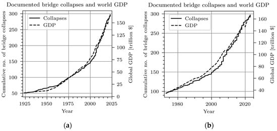
Figure 1.
Correlation between bridge collapses [2] and world GDP [3] in the last 100 (a) and 40 years (b).
Without systematic inspections, monitoring, timely interventions, and implementation of new technologies, even nominally robust systems gradually deteriorate, culminating in higher collapse rates. Recognising this linkage justifies the current research efforts into new technologies, such as structural health monitoring (SHM), finite element model updating (FEMU), and bridge weigh-in-motion (B-WIM), especially as transport networks become ever more extensive and critical to economic development. Tackling these issues requires better and more robust predictions of bridge behaviour. One approach that copes with these requirements is FEMU, where finite element (FE) models are updated to match the analytical and measured responses.
In structural dynamics, FEMU traces back to the early efforts of reconciling FE simulations with measured vibration data to refine predictions of real-world structural behaviour. Mottershead and Friswell [4] conducted a deep survey on the topic, systematising key approaches for parameter selection, objective function formulation, and optimisation strategies. Early on, most FEMU applications focused on natural frequencies and mode shapes to capture global structural responses. Over time, researchers recognised that purely vibration-based data sometimes lacked sensitivity to localised parameters (e.g., small-scale stiffness or boundary nuances). This realisation gradually led to new data types, such as displacements and strains [5,6,7,8,9,10], being integrated into the FEMU process, helping to address the inherent limitations of purely modal data. Building on these foundations, the current generation of FEMU techniques harnesses large-scale test data under various loading scenarios. One promising approach is using measured influence lines (ILs). IL-based approaches reflect global and local responses with minimal instrumentation, allowing for more precise FEMU. Using ILs in FEMU can more accurately describe local boundary conditions, subtle stiffness variations, and stress distribution patterns.
The literature proposes various signal-processing and inverse analysis techniques to extract an IL from measured bridge responses under moving loads: spatial-domain, frequency-domain, and decomposition-based methods. O’Brien et al. [11] introduced a bridge IL identification method through spatial domain modelling. This approach quantifies the connection between vehicle axle load, IL coefficients, and bridge response at different vehicular positions. Alternatively, one can achieve response normalisation in the frequency domain, restoring the IL using the inverse Fourier transformation. Yan & Yuen [12] developed a method that utilises static response transfer ratio functions to identify IL from a probabilistic frequency domain viewpoint. Similarly, Frøseth et al. [13] identified IL in the frequency domain based on the principle that the convolution of the moving load and IL results in the bridge response. An adaptive enhanced variational mode decomposition (AEVMD) method was presented for extracting the bridge’s quasi-static response [14]. This method combines the pre-processed conjugate gradient least squares (PCGLS) algorithm to determine the IL. Although both spatial and frequency domain methods effectively create mathematical models for IL identification, they remain vulnerable to dynamic interference. In contrast [15], a non-linear optimisation approach, drawing from a substantial number of random vehicles in traffic flow with unknown axle loads to define the shape of the influence line, has a notable advantage since the inherent dynamic responses of both the bridge and vehicles influence the IL shape less. This can skew results based solely on a limited number of pre-weighed vehicles. This paper follows this aspect of leveraging continuous advances in sensor technology, signal processing, and data-driven optimisation to enhance IL-based FEMU, ensuring more precise and robust methodologies for bridge health monitoring and structural safety assessment.
This paper builds on previous work on using strain ILs obtained from B-WIM measurements. Strain ILs are essential for B-WIM algorithms to calculate accurate axle loads [15]. Algorithms have been developed to calculate strain ILs from all heavy gross vehicle crossings. Hundreds are statistically evaluated to obtain reliable information on bridge performance under moving loads [16]. In the past, these B-WIM-calculated strain ILs have already been used to calibrate the analytical models of simple short-span bridges. In this study, we first enhanced the strain IL calculation methodology to account for quantities better suited to bridge analyses. Then, we used the results to update the case study bridge and compared the FEMU results with more traditional frequency and mode shape-based FEMU results. For the FEMU, we replaced the traditional methods, such as Bayesian model updating and residual minimisation, with the EDMF methodology. Lastly, we validated the FE model response with measured displacements under calibration vehicle passages.
The novelty of the proposed method lies in integrating measured strain ILs, derived from B-WIM data, into the FEMU process, representing an important advancement over traditional approaches that rely solely on modal parameters, like frequencies, MAC values, or on maximum strains under traffic load. It offers a cost-effective alternative to displacement-based methods, which were independently validated to yield comparable results in terms of response prediction. Methodologically, this study replaces more demanding Bayesian updating and residual minimisation with the error-domain model falsification (EDMF) approach. This falsification-based framework identifies plausible variable values of the FE model by systematically eliminating FE models that fail to match experimental data within defined uncertainty bounds. This makes it more robust to systematic uncertainties and model biases and increasingly recognised for its accuracy and practical effectiveness in structural identification. These methodological contributions not only simplify the FEMU process, but also enhance the role of B-WIM in structural identification and long-term SHM.
2. Materials and Methods
2.1. Description of the Case Study Bridge
The case study Tomačevo roadway bridge was built in 1982 and crosses the Sava River near the Slovenian capital Ljubljana (LJ). Its superstructure is a seven-span continuous post-tensioned double-T section supported by circular piers on deep foundations (Figure 2).
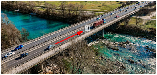
Figure 2.
Aerial view of the Tomačevo bridge, with an arrow indicating the traffic flow in the Ljubljana (LJ) direction.
The bridge consists of two parallel independent structures. The right one (Figure 3a,b inside the red rectangles) carries traffic in the LJ direction and the left one in the opposite (northeast) direction. This paper focuses on the right structure, denoted as the bridge throughout this paper.

Figure 3.
View under the Tomačevo bridge towards LJ (a) and opposite direction (b). Red arrows indicate traffic direction and red rectangles the right structure, considered in this paper.
The superstructure was cast in place with sliding formwork technology. Cross girders at the abutments connect longitudinal main girders. The bridge is bounded by modular expansion joints at both abutments, where the superstructure is supported by guided unidirectional pot bearings. The superstructure passes continuously above piers, supported by round elastomeric bearings. No major rehabilitation works have been performed on the bridge since its completion, apart from the expansion joint replacement in 1990 and the asphalt layer and steel safety barrier replacement in 2018.
The bridge is in good condition, with typical damages and defects, such as local insufficient cover layer and consequent spalling of concrete, clogged expansion joints, and corroded bearings. Drainage is inadequately implemented and maintained in several places, especially near the abutments, which has caused accelerated deterioration of concrete and bearings, as shown in Figure 4.

Figure 4.
Water leakage at the abutments (a) and a corroded guided unidirectional pot bearing (b).
Side, plan, and cross-section views of the bridge are shown in Figure 5. Typical elements are labelled with abbreviations, such as MG1, representing Main Girder 1, CG, representing the Cross Girder, and similar to other elements, described in more detail in Table 3.
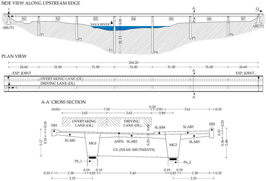
Figure 5.
Plan view, side view, and cross-section view of the bridge. Typical elements are labelled with abbreviations, described more in detail in Table 3.
2.2. Measurements
The Tomačevo bridge is a B-WIM and SHM living-lab facility designed to develop and test new technologies, sensors, and methods. The measurements setup on the bridge varied over time, but for this study, the following sensors, shown in Figure 6, were considered:
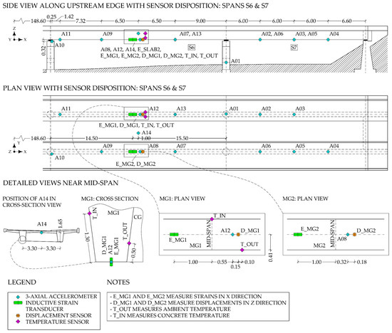
Figure 6.
Disposition of the sensors used in this paper. Typical elements are labelled with abbreviations, described more in detail in Table 3.
- Fourteen Dewesoft-type IOLITEi 3xMEMS-ACC tri-axial MEMS accelerometers (Dewesoft, Trbovlje, Slovenia) measuring the ambient and traffic-induced vibrations and to determine the modal parameters of the bridge;
- Two inductive strain transducers (denoted in the paper as B-WIM sensors) measuring traffic-induced strains on both girders, and to obtain input for the B-WIM measurements;
- Two linear variable differential transformers (denoted as LVDTs or. displacement sensors) (HBK, Darmstadt, Germany) measuring traffic-induced vertical displacements on both main girders;
- Two temperature sensors, T_OUT (Dewesoft, Trbovlje, Slovenia)measuring environmental temperature and T_IN, measuring the temperature approximately 5 cm inside the main girder MG1.
DewesoftX 2023.5 data acquisition software [17] was used for data recording with a 500 Hz sampling frequency.
Besides the sensors that measure the mid-span strains on main elements such as girders and slabs, B-WIM systems generally require additional sensors to detect the axles and calculate the vehicle’s speed. In the lateral direction, they are installed on the elements and locations close to the vehicle’s wheel track to capture clear spikes, representing individual axles. One pair of such strain sensors was installed on the SLAB1 and one on the SLAB2 element.
2.2.1. Strain and Displacement Measurements Under the Calibration Vehicle Crossings
Strains and displacements were measured in May 2024 at night to avoid congestion and minimise the presence of other vehicles on the bridge. The environmental conditions were similar both nights; for the time of the experimental campaign, the difference between the measured average temperatures of the first (18.2 °C) and second (17.7 °C) nights was 0.5 °C. Two statically pre-weighed calibration vehicles were used (Figure 7), a tri-axle rigid truck, denoted as V1, and a two-axle tractor with a three-axle semi-trailer, denoted as V2.

Figure 7.
Calibration vehicles: V1 (a) and V2 (b).
Both vehicles were fully loaded on the first night and empty on the second night. Their axle loads, spacing, and gross vehicle weight (GVW) are shown in Table 1.

Table 1.
Axle loads, axle spacing, and gross vehicle weights (GVW) of the calibration vehicles.
Each vehicle passed the bridge in the driving lane ten times at 90 km/h, five times at 70 km/h, and three times at 30 km/h. Two trucks performed seventy-two passages in two nights, which is approximately 50% of the recommended passages by COST 323 [18].
Then, the B-WIM analysis used the measurement result from the E_MG1 and E_MG2 sensors, and the strain IL was extracted. No displacement IL was extracted since the measured displacement response under the calibration vehicles was only used to validate the updated FE model, and not in the B-WIM and FEMU parts.
2.2.2. Extraction of the Strain Influence Line (IL) from the Strain Measurements
B-WIM refers to a method that uses an instrumented bridge or culvert to weigh-in-motion the passing vehicles. The B-WIM analysis is an inverse-type problem where the structural response (mid-span strains) is measured and the traffic load causing this response is calculated [19]. Most operational B-WIM algorithms, including the one in this study, work on static assumptions and follow the principles proposed by Moses [20]. The key parameter in the B-WIM analysis is the IL, a function that describes the response of a structure at a given point under a moving unit load. IL illustrates how various load effects, like displacements and strains, change under the moving traffic loads.
Several methods of calculating ILs exist [21]; the method used in this paper has been described in detail in [16]. The following is a short recap of the method and the adjustments required for its use in FEMU. The goal of B-WIM is to solve a system of equations, defined in (1) as:
where s(tj) is the average value of the strain signals from sensors at M different times, Ai is the unknown axle weight, I(x) is the known strain IL, vi is the measured axle velocity, ti is the arrival time of an individual axle, N is the number of axles, and M is the number of measurements, which must be greater than or equal to N. The strain IL is specified in advance. Thus, the equation is linear in the unknown terms, meaning that relatively simple methods suffice to obtain the axle weights.
The same equation can be used to calculate the strain IL by treating the function I(x) as an unknown, in addition to axle loads. Cubic splines are used to model the strain ILs. Splines are curves of the third order, smooth in derivatives and continuous in second derivatives, thereby matching the characteristics of observed strain ILs. The solved system is not linear in the unknown terms, necessitating iterative methods.
Figure 8 demonstrates the principle of strain IL modelling for a hypothetical three-span bridge, for the strain sensor located at the mid-span of the inner span. The strain IL is defined by the three types of points. The white points represent supports, the abscissas are defined by geometry, and the ordinates are 0. The exception is point M, located at the measurement point and whose ordinate is also optimised. The grey points define the radius d/2 of the rounded cap that improves the fit between the measured and modelled responses. Finally, the optional black points A through F can fine-tune the match. Their x-coordinates are selected, and y-coordinates are optimised. The ordinates of the curve between the control points are obtained with cubic spline interpolation.
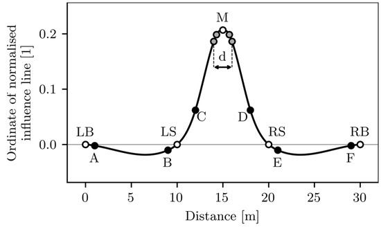
Figure 8.
Hypothetical three-span bridge strain influence line (IL), approximated with cubic splines (adapted from [16]). The ordinates of the IL are obtained with cubic spline interpolation between the white (LB, LS, M, RS, RB), grey and black (A, B, C, D, E, F) control points.
This study required an adaptation to the original method for calculating the strain IL. As this technique can be applied to random traffic, monitoring its shape through time and detection allows for possible changes in bridge behaviour [16]. Since the axle loads of the vehicles from random traffic are unknown, the absolute strain IL value cannot be calculated. Instead, the strain IL is normalised so that the integral between points LS and RS is equal to 1, and the “raw” axle loads, calculated from the equation, adapt to this. Finally, one or more calibration vehicles with known axle loads cross the bridge several times. The ratio between raw and actual loads is calculated for each run, and the mean value of all results is taken as a calibration factor that converts raw into actual loads.
Calculating the strain IL with known axle loads, as in this study, allows for avoiding normalisation, as the actual influence of a unit axle on the bridge is needed. The known axle loads of the calibration vehicles were taken, and the strain IL height adapted itself during calculations.
Strain ILs were extracted separately for vehicle type and load (V1F, V1E, V2F, and V2E) and for vehicle speed (30, 70, and 90 km/h). Overall, 12 strain ILs were generated for each sensor. Figure 9 shows the strain ILs for sensors E_MG1 (a) and E_MG2, with blue, red, magenta, and green colours denoting V1F, V1E, V2F, and V2E vehicles, respectively. The mean (µ) and mean ± standard deviation (µ ± σ) values are shown with dashed and grey lines, respectively.

Figure 9.
E_MG1 (a) and E_MG2 (b) strain ILs showing the (in)dependence of vehicle load and type.
Similarly, Figure 10 shows the generated strain ILs for sensors E_MG1 (Figure 10a) and E_MG2 (Figure 10b), with red, green, and blue colours denoting 30, 70, and 90 km/h speeds, respectively.

Figure 10.
E_MG1 (a) and E_MG2 (b) strain ILs showing the speed (in)dependence.
Figure 9 and Figure 10 indicate that vehicle type, load, and speed have a minimal impact (less than ±5% deviation of the maximum strain IL values, compared with the maximum values of the mean strain IL) on the strain IL’s shape and magnitude. Consequently, the mean values of E_MG1 and E_MG2 strain ILs were used for the FEMU.
2.2.3. Ambient and Traffic-Induced Vibration Test
Operational modal analysis (OMA) was performed from the 60 min long signal, captured after the last passage of the calibration vehicle, the second night at 3:00 AM. Only a few passenger cars crossed the bridge in that time window. ARTeMIS Modal Pro 7.2 software [22] with the enhanced frequency domain decomposition (EFDD) method was used to estimate the modal parameters. The 66% overlap and 4096-point data samples resulted in approximately 0.06 Hz frequency resolution. Figure 11 shows the singular spectral density values for the limited range from 0 to 10 Hz. The coloured markers denote the detected modes used in the FEMU study, and the nearby text denotes the frequency values.

Figure 11.
Singular spectral density values. Coloured markers denote the detected modes used in the FEMU study.
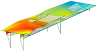
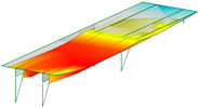
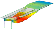
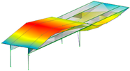
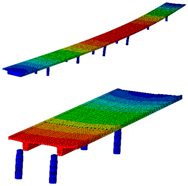
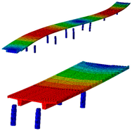
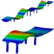
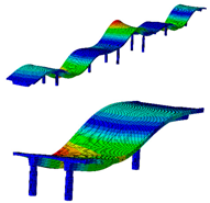
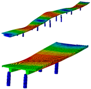
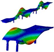
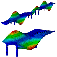
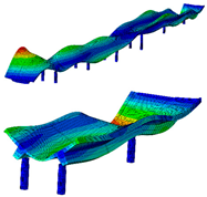
Eight modes were identified and considered in the FEMU. Modes are named by their shape (B for bending, T for torsion), direction (Y for movement in Y, Z for movement in vertical direction), and harmonics (1 for first harmonic, etc.). Mode name ‘B-Y-1’, for example, represents the first bending mode in the Y direction. Not all modes, represented by evident peaks, were considered. Their significance was decided based on their complexity, shape observation, modal assurance criterion (MAC) value, ability to distinguish them from the nearby modes, and whether they could be automatically detected and paired with measured modes. Table 2 shows natural frequencies and corresponding mode shapes from the ambient and traffic-induced vibration test. Red indicates the highest, and blue the lowest displacement magnitudes. Semi-transparent grey colour denotes the undeformed geometry.

Table 2.
Natural frequencies and corresponding mode shapes from the ambient and traffic-induced vibration test. Red indicates the highest magnitude of displacements, while blue indicates the lowest. Semi-transparent grey colour denotes the undeformed geometry.
Figure 12 shows the auto-modal assurance criterion (Auto-MAC) matrix for the experimental mode shapes.
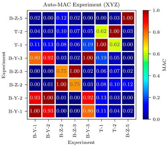
Figure 12.
Auto-MAC matrix for the experimental mode shapes.
2.3. Finite Element (FE) Model
The bridge FE model was developed in Abaqus/CAE 2023 [23] software. All structural elements of the superstructure and piers were modelled using 20-node quadratic (C3D20R) hexahedral and 8-node linear (C3D8R) hexahedral elements, respectively. The approximate global mesh size was set to 0.50 m. Two analyses were conducted: modal analysis for extracting natural frequencies and mode shapes, and static analysis to determine the strain ILs. A 3D view and a detailed view of the pier–main girder and main girder–cross girder connections are shown in Figure 13a–d. Throughout this paper, the FE model, with properties from the design documentation, is denoted as the initial FE model.
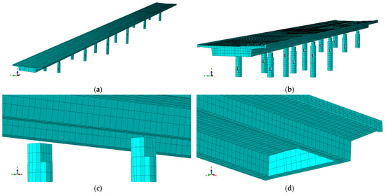
Figure 13.
Finite element (FE) model of the bridge in the Abaqus/CAE 2023 software: 3D view of the entire bridge (a,b), detailed view near pier–main girder connection (c) and detailed view of the cross girder near abutments (d).
2.3.1. Geometry and Materials
The FE model was based on the geometry outlined in the design documents [24,25,26,27]. No in situ measurement data were used to construct the initial FE model. The edge beams and slab geometry were minimally simplified to design the finite element mesh. An isotropic elastic material was used for all elements. The material properties according to the design documentation [24,25,26,27] are shown in Table 3. Young’s modulus and density for selected elements were modified to consider the element’s weakening (holes in the SLAB5 element) and the effect of the attached non-structural elements.

Table 3.
Material properties of structural elements according to design documentation [24,25,26,27].
Table 3.
Material properties of structural elements according to design documentation [24,25,26,27].
| Element | Abbreviation | Young’s Modulus (GPa) | Poisson Ratio | Density (t/m3) |
|---|---|---|---|---|
| Asphalt | ASPH | 8.00 | 0.35 | 2.582 |
| Edge beam 1 | EB1 | 31.00 | 0.20 | 2.710 |
| Edge beam 2 | EB2 | 31.00 | 0.20 | 2.580 |
| Main girder 1 | MG1 | 35.00 | 0.20 | 2.500 |
| Main girder 2 | MG2 | 35.00 | 0.20 | 2.500 |
| Slab 1 | SLAB1 | 35.00 | 0.20 | 2.500 |
| Slab 2 | SLAB2 | 35.00 | 0.20 | 2.500 |
| Slab 3 | SLAB3 | 35.00 | 0.20 | 2.500 |
| Slab 4 | SLAB4 | 35.00 | 0.20 | 3.573 |
| Slab 5 | SLAB5 | 14.59 | 0.20 | 1.177 |
| Pier (bottom part) 1 | PIER_BOTTOM | 31.00 | 0.20 | 2.500 |
| Pier (upper part, bearing region) 1 | PIER_TOP | 34.00 | 0.20 | 2.500 |
| Cross girder | CG | 35.00 | 0.20 | 2.500 |
1 PIER_BOTTOM represents the bottom parts, and PIER_TOP represents the top parts (bearing region) of all pier pairs: P1, P2, P3, P4, P5, and P6.
2.3.2. Interactions and Boundary Conditions
Piers were connected to the superstructure with elastomeric bearings modelled as wires (spring–dashpot assemblies). “Cartesian + Rotation” connector sections were assigned to these wires (assemblies), which connected reference points on the pier–girder contact surfaces. Stiffness properties were obtained from the design documentation, and their stiffness properties were obtained from the design documentation [27] and are shown in Table 4. Unidirectional pot bearings, which connected the superstructure to the abutments, were not modelled as wires. Instead, the bearing surface was assigned a boundary condition with restrained movements in the Y and Z directions. A fixed boundary condition, which restrains displacements in all directions, was assigned to the bottom surfaces of all piers.

Table 4.
Properties of bearings according to design documentation [27].
2.4. Comparison of the Initial FE Model and Measurements
2.4.1. Strain IL
Strain ILs were calculated for longitudinal (E11) strains at the E_MG1 and E_MG2 positions. Since only the driving lane vehicle crossings were considered, the strain ILs were obtained with two pairs of 0.5 kN point loads (representing the vehicle wheels) varied across the last three spans, starting at the beginning of S5 and ending at the end of S7, at the expansion joint. The strain ILs were calculated for point loads spaced approximately 1.0 m apart, representing 92 static analyses required to extract each strain IL. Lastly, the modelled strain IL was discretised to 0.01 m with a cubic interpolator for the comparison with the measured strain IL. Figure 14 displays the E_MG1 (a) and E_MG2 (b) strain ILs of the initial FE model, the related measured strain ILs, and the differences between the two.

Figure 14.
Strain ILs of the initial FE model and measured strain IL for E_MG1 (a) and E_MG2 (b).
As expected, the modelled strain ILs overestimated the measured ones, with the peaks exceeding the measured values by approximately 45% for both sensors.
2.4.2. Natural Frequencies and Mode Shapes
Table 5 shows the natural frequencies and mode shapes of the initial FE model. Only the modes considered for the FEMU are shown. Each has two figures. The upper shows the entire structure, and the lower shows the last two spans (S7, S8). Since the accelerometers were only installed in spans S7 and S8, the measured mode shapes are available only for those two spans. The purpose of the lower figure is to easily compare the modelled and measured responses in spans S7 and S8, as shown in Table 2.

Table 5.
Natural frequencies and mode shapes of the initial FE model considered for the FEMU. The red colour indicates the highest, and blue the lowest displacement magnitude.
2.5. Finite Element Model Updating (FEMU): Error-Domain Model Falsification (EDMF)
For the FEMU, the EDMF methodology was employed instead of traditional approaches such as Bayesian model updating or residual minimisation. Introduced in 2013 for bridge load testing [28], EDMF is a structural identification methodology that leverages the falsification concept. Outlined by [28], it has deep roots in scientific methods, formalised in the 1930s by Karl Popper, who asserted that scientific models cannot be entirely verified by data, but can only be falsified. Using this framework, EDMF determines plausible values for FE model variables based on experimental field data and defined uncertainty levels. The methodology involves creating various FE model instances, each characterised by a unique set of variable values. These are then assessed by comparing the model’s predictions with actual sensor data collected during experiments. Models that deviate beyond the set uncertainty thresholds are deemed falsified, narrowing the range of potential variable values.
According to [29], using falsification thresholds makes EDMF robust against the assumptions typically made about the correlation of uncertainties and incorporates adjustments for model biases based on engineering heuristics. This approach has been proven to offer more accurate identification and predictions, particularly where there is considerable systematic uncertainty, outperforming traditional methods like Bayesian model updating and residual minimisation. Its efficacy and growing acceptance are evidenced by its application in nine bridge-related studies, four on buildings, and two on geotechnical projects from 2015 to 2022 [29].
3. Results
3.1. Sensitivity Study
A deterministic sensitivity study was performed to understand the impact of individual structural elements and the boundary conditions on the natural frequencies and strain ILs. Based on its results, variables to be updated were selected. List of variables considered in the sensitivity analysis with the description is shown in Table 6.

Table 6.
List of variables considered in the sensitivity analysis with the description.
3.1.1. Natural Frequencies
The objective function measures the similarity of modelled and measured natural frequencies. The lower it is, the lower the difference between the modelled and measured frequencies. It is defined as:
where and are the ith matching mode pair of the natural frequencies from the FE model experiment, respectively. n is the overall number of natural frequencies considered. According to [30], this is the “normalised” type objective function.
3.1.2. Strain IL
The objective function measures the difference between the modelled and the mean measured strain IL. The lower it is, the more similar the compared strain ILs are. is defined separately for E_MG1 and E_MG2. Despite comparing two vectors (strain ILs), it is a scalar value. By definition, it is equal to the root-mean-square error (RMSE):
where is the j-th ordinate of the modelled strain IL and is the j-th ordinate of the mean measured strain IL . m is the number of ordinate values considered and is the mean measured strain IL (from all passages). JIL can be interpreted as an average difference between the modelled and measured strain IL.
The sensitivity study results for the variation in the boundary conditions (bearings) and structural elements Young’s modulus on the relative change in the objective function are shown in Figure 15. Those for the variation of boundary conditions (bearings) and structural elements Young’s modulus on the relative change of the objective function and are shown in Figure 16a,b.
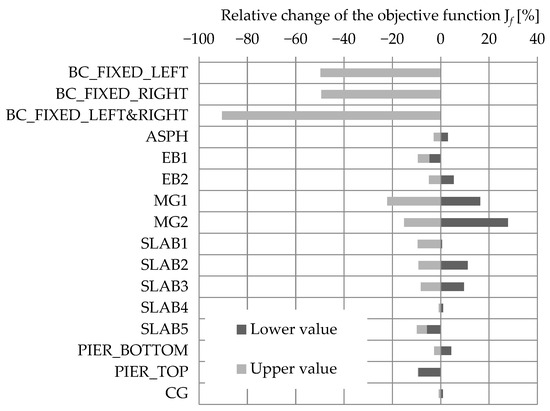
Figure 15.
The sensitivity study results for the variation in boundary conditions (bearings) and structural elements’ Young’s modulus values on the relative change in the objective function .
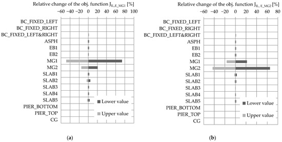
Figure 16.
The sensitivity study results for the variation in boundary conditions (bearings) and structural elements’ Young’s modulus values on the relative change in the objective function (a) and (b).
Based on the sensitivity study results, it was decided to update the boundary conditions and Young’s modulus of structural elements. For the mass, it was decided to estimate it as accurately as possible and keep it fixed to ensure that its increase did not decrease stiffness and vice versa (for the frequency-based FEMU). The Young’s modulus values of MG1 and MG2 were updated through “Young’s modulus adjustment factors” and . Those factors were defined as a correction factor, relative to the designed Young’s modulus (shown in Table 3). A value of 1.00, for example, denotes no change in the Young’s modulus and value of 1.20 denotes a 20% increase in the designed Young’s modulus. All other structural elements were grouped into the ‘OTHER’ group, and their Young’s modulus was updated by the same percentage through the Young’s modulus adjustment factor.
It is crucial to note that the objective of FEMU, as outlined by [28], is not to adjust FE model variables to align the predicted and measured values better. Instead, model-based system identification employs physics-based models to deduce variable values. Consequently, the variables chosen for FEMU do not reflect the actual properties of structural elements, such as Young’s modulus (adjustment factor). Instead, they should be viewed to consolidate the structural properties into a single variable. This distinction is important to remember, particularly when analysing the absolute values of the updated variables.
3.2. Updated FE Model
This chapter provides a comprehensive summary of the EDMF results, commencing with the frequency-based EDMF as illustrated in Figure 17, followed by the MAC-based EDMF depicted in Figure 20. Subsequently, a combined analysis of frequency- and MAC-based EDMF is shown in Figure 21. Finally, the strain-based EDMF results are presented in Figure 22. In these figures, experimental values are denoted by red markers, red horizontal lines indicate thresholds, candidates are represented in blue, and models that have been falsified are noted in grey. RMSE and MAC values are not measured, but calculated from modelled and measured responses. Therefore, the experimental values were denoted as 0 for RMSE values and 1.00 for MAC, representing the perfect match between the FE model and measurements.
3.2.1. Frequency-Based EDMF
In the frequency-based EDMF shown in Figure 17, all eight frequencies were considered. Thresholds for all frequencies were set as a multiplier of the experimental values; in this case, the [0.80, 1.20] interval, representing the as the lower bound and as the upper bound. The candidates had frequencies within ±20% of the measured values for this case. For a good correlation between the FE model and measurements, the relative difference between frequencies should be less than 5% [31]. In the initial phases of this study, it was necessary to apply threshold values somewhat higher than usual to identify viable candidates. While this may seem unrealistic, it was essential to obtain any candidates at all. Although the thresholds were subsequently reduced to 5% or less in later steps, we retained this stage to illustrate how the process of FEMU using EDMF was structured to facilitate the identification of the mode with the greatest deviation, and that finally guided us towards understanding the underlying cause. Note that, although strain IL-based (RMSE values) and MAC-based outputs (MAC values) are shown in this EDMF plot, in this case, they do not determine the candidates because of the large thresholds.

Figure 17.
Frequency-based EDMF results. Experimental values are denoted by red markers, red horizontal lines indicate thresholds, candidates are represented in blue, and models that have been falsified are noted in grey.
B-Y-1 frequencies were underestimated and B-Z-3 overestimated compared with the measurements, as shown in Figure 17. Analysis of the EDMF’s outputs was performed, where mean values of the modelled frequencies were compared with the experimental values, as shown in Figure 18.
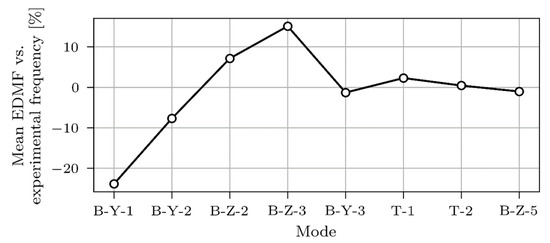
Figure 18.
Difference between mean modelled (EDMF) and experimental frequencies.
The greatest absolute deviation between the mean modelled and measured values of frequencies was observed for B-Y-1 and B-Z-3 (Figure 18). Recalling the sensitivity study results, fixed boundary conditions importantly reduce the objective function for natural frequencies and could significantly influence the B-Y-1 frequency. Contrary, fixed boundary conditions have a negligible effect on the strain ILs’ objective functions. In the following, all analyses were performed on the FE model with fully fixed boundary conditions, where all degrees of freedom were constrained for bearings at both abutments.
The investigation of B-Z-3 overestimation revealed that the reason was the unreliable mode pairing strategy, which often paired the modelled B-Z-3 with the experimental B-Z-4 mode. By using the EDMF approach, it is possible to identify suspicious outputs caused by, for example [32], faulty sensors. A similar process was followed in this study, where the B-Z-3 mode was eliminated for all following analyses. Although still present in the EDMF plots, the B-Z-3 mode was excluded by setting the falsification threshold range for the B-Z-3 frequency between the minimum and maximum values of the modelled frequencies, allowing all FE models to pass through the B-Z-3 frequency thresholds. Figure 19 shows the frequency-based EDMF analysis on the FE models with fully restrained bearings at abutments and with B-Z-3 frequency eliminated. The threshold for all frequencies was set to [0.975, 1.025], allowing the frequencies to deviate to ±2.5%.

Figure 19.
Frequency-based EDMF results. B-Z-3 frequency is not considered. Experimental values are denoted by red markers, red horizontal lines indicate thresholds, candidates are represented in blue, and models that have been falsified are noted in grey.
Considering fully restrained bearings at the abutments was essential for improving the B-Y-1 frequency results. This approach showed a minimal impact on the E_MG1 and E_MG2 strain IL responses, as illustrated in Figure 18. Previous studies, such as those referenced in [30,33], have also documented limited or restrained movements in bearings during ambient vibration tests. Although this effect was not measured directly, it was observed that clogged expansion joints and corroded bearings, as shown in Figure 4, limit movement, which is contrary to the original design specifications. Therefore, the assumption of fully restrained bearings at the abutments was considered reasonable, but should be studied in more detail in future research, for example, to model them as springs and change their stiffness gradually.
After considering fixed boundary conditions and eliminating the B-Z-3 frequency, the frequency-based EDMF results indicated large ([1.00, 1.50]) and ([0.90, 1.40]) ranges, while was equal to 1.00. Additionally, some candidates with a high value had a small value, which is not in line with the engineering judgement. Given that MG1 and MG2 are visually in similar conditions, it is expected that and would be comparable and higher than due to the many prestressing tendons. Those results are similar to the findings from another viaduct [34], where some candidates had a high–low stiffness trend for main girders, despite expectations that they would be comparable. After additional measurement data were added to the EDMF, that trend aligned with the engineering expectations.
3.2.2. MAC-Based EDMF
Figure 20 shows the MAC-based EDMF results. For the well-correlated modes, the MAC values should be greater than 0.90 [31], and for ‘acceptable’, 0.80 [35]. For MACs, the upper value of the thresholds was set to 1.00 for all modes, representing the scenario of perfectly similar modelled compared with the measured mode shape. The lower thresholds were set to 0.80 for all modes except for B-Z-3, which was, as already mentioned, removed from all analyses.

Figure 20.
MAC-based EDMF results. Experimental values are denoted by red markers, red horizontal lines indicate thresholds, candidates are represented in blue, and models that have been falsified are noted in grey.
The MAC-based EDMF results fell into ranges [1.50, 1.60] for , [1.10, 1.50] for , and [0.80, 1.10] for .
3.2.3. Frequency & MAC-Based EDMF
The MAC values of some modes never exceeded the 0.90 value. There may have been several reasons for this [36], the sparse and/or improperly distributed sensor layout concerning the geometric complexity of the tested structure [37] being among the most likely. Despite that, it was expected that MAC criteria would improve results once added to the frequency-based EDMF. Particularly because the low MAC values also indicated incorrectly paired modelled and measured modes. As such, it would complement the frequency-based EDMF with more reliable candidates. Figure 21 shows the frequency and MAC-based EDMF results. The threshold for frequencies was set to [0.95, 1.05]. The upper thresholds for MAC were set to the absolute value of 1.00, and the lower thresholds to 0.78.

Figure 21.
Frequency and MAC-based EDMF results. Experimental values are denoted by red markers, red horizontal lines indicate thresholds, candidates are represented in blue, and models that have been falsified are noted in grey.
The frequency and MAC-based EDMF produced a narrower range for ([1.20, 1.30]) and ([1.10, 1.30]), compared with the frequency-based EDMF. Both values were comparable and higher than ([0.80, 1.00]), which is in line with engineering expectations.
3.2.4. Strain IL-Based EDMF
Figure 22 shows the strain IL-based EDMF. The bottom thresholds for strains were set to 0, representing the perfect match between the measured and modelled strain IL. The upper thresholds were set iteratively, such that three candidates were obtained. All candidates had RMSE E_MG1 and RMSE E_MG2 values lower than 96% for all FE models.

Figure 22.
Strain IL-based EDMF results. Experimental values are denoted by red markers, red horizontal lines indicate thresholds, candidates are represented in blue, and models that have been falsified are noted in grey.
The final candidates produced by the strain-based EDMF had and values in the narrow range of [1.30, 1.40] and 1.50, respectively. They are both comparable with the results from the Ravbarkomanda viaduct study [34], where the stiffness of the main girders increased by up to 50%. The values of were in the range [1.20, 1,50].
3.2.5. Comparison of EDMF Results
Table 7 presents outputs; RMSE values for E_MG1 and E_MG2 sensors, and natural frequencies and mode shapes for the initial FE model and all four EDMF analyses. The measured values are added for comparison. ‘Bottom’ and ‘Upper’ denote both range thresholds the candidates provided. The RMSE values for both sensors were set to 0, and the MAC values for all mode shapes were set to 1.00. For each output, the cell value in a row that deviated most from the measured value is coloured red, and the one closest to the measured value is green. B-Z-3 frequencies and mode shapes are coloured grey because they were not considered in the EDMF study. Again, the results of all EDMF studies were calculated in the FE model with all restrained degrees of freedom at the ABUT1 and ABUT2 bearings. In contrast, the initial FE model enabled longitudinal movements.

Table 7.
Outputs: measured, initial FE mode, after frequency-based EDMF, after MAC-based EDMF, after frequency and MAC-based EDMF, and after strain IL-based EDMF. Red colour denotes the greatest and green the lowest deviation from the experimental values. Grey colour denotes the B-Z-3 mode that was not considered in the EDMF study.
The comparison of the EDMF results in Table 7 yielded the following conclusions:
- Setting bearings ABUT1 and ABUT2 to fixed improved the B-Y-1 and B-Y-2 modelled vs. measured frequency values;
- Frequency-based EDMF primarily improved the frequency values; a minor improvement was also seen for E_MG1 and E_MG2 strain ILs. The MAC values decreased;
- MAC-based improved MAC values, improvement in E_MG1 and E_MG2 strain ILs was greater than that in the frequency-based EDMF;
- Frequency and MAC-based EDMF improved frequencies and MACs, closely matching the results of frequency-based EDMF (for frequencies) and MAC-based EDMF (for MAC values), while both strain ILs did not align more closely with the measured ones;
- Strain-based EDMF only improved both strain ILs. Frequency and MAC values were even worse than for the initial FE model.
Table 8 presents the updated variables for all EDMF studies performed. The initial values of 1, obtained from the initial FE model, are added for comparison.

Table 8.
Comparison of EDMF results: updated variables.
Comparing the values from Table 7 and Table 8 yielded the conclusion that combining frequencies and MACs into EDMF was reasonable because it has significantly narrowed the range of the candidates’ variables. The updated approximately 25 and 20% increases in the MG1 and MG2 main girders’ stiffnesses and 10% decrease in the stiffnesses of all other elements are also in line with the expectations. Some updated MAC values are still lower than 0.90, and it should be noted that future research is needed to investigate the cause. The strain IL-based EDMF narrowed the MG1 and MG2 stiffness increases to more reasonable values of 35 and 50%. The range, however, remained wide as the E_MG1 and E_MG2 strain ILs were not sensitive to OTHER elements.
The strain IL-based EDMF generally resulted in approximately 10–15% higher values of frequencies (Figure 22) than those from the frequency and MAC-based EDMF (Figure 21) or measured ones. A similar trend can be seen for the RMSE values from the frequency and MAC-based EDMF. They were higher than the strain IL-based EDMF values, because the MG1 and MG2 stiffnesses were underestimated. Figure 23 compares the strain ILs of the initial FE model with the frequency and MAC-based and strain IL-based updated models for E_MG1 (Figure 23a) and E_MG2 (Figure 23b).

Figure 23.
E_MG1 (a) and E_MG2 (b) strain ILs: comparison of measured, initial, frequency and MAC-based, and strain IL-based updated models.
The initial FE model overestimated the maximum modelled E_MG1 IL strains by 43% compared with the measured values. The frequency and MAC-based updated FE model overestimated the measured strains by 32%, and the strain IL-based FE updated model by 12%. For E_MG2 IL strains, the corresponding overestimations were 44%, 33%, and almost none, respectively.
Discrepancies between the modal (frequency, MAC)-based and static (strain, displacement)-based FEMU have already been reported, for example, by [30,38,39]. Despite using the advanced FE model with 3D finite elements and reliable measurement data in a controlled environment, this study could not eliminate these discrepancies. A potential cause could be that we measured a more global response with acceleration than with strain or displacement measurements under traffic load. The captured mode shapes, shown in Table 2, showed global behaviour in all directions, while for strain and displacement measurements, the bridge mainly deformed only in the vertical direction in S5, S6, and S7 spans. This means that the structural elements contributed differently to the modal and the static (strain, displacement) responses, which was already shown in the sensitivity analysis. This should be studied more in the future, along with the impact of non-structural components, like railings and pipes, and assumptions regarding mass.
3.3. Validation of the Updated FE Models with Measured Strains and Displacements Under Calibration Vehicle Passages
3.3.1. Strains
This section compares the measured and modelled E_MG1 and E_MG2 strains under V2_F vehicle crossings. The entire strain histories are presented, and not just the strain ILs for the E_MG1 and E_MG2 sensors. Figure 24 and Figure 25 compare the responses of E_MG1 and E_MG2 sensors, respectively. First, the strain records of three crossings at approximately 30 km/h are shown; the colours denote the exact measured speed. The mean of the three maximum values is shown with a marker. Then, three responses are added for the initial ( = 1.00, = 1.00, = 1.00), frequency and MAC-based (one of the candidates with = 1.20, = 1.10, = 1.00), and strain IL-based updated FE models (one of the candidates with = 1.30, = 1.50, = 1.40).

Figure 24.
Comparison of E_MG1 strains under V2_F passages: measurements (30 km/h), initial, frequency and MAC-based, and strain IL-based updated FE models.

Figure 25.
Comparison of E_MG2 strains under V2_F passages: measurements (30 km/h), initial, frequency and MAC-based, and strain IL-based updated FE models.
The strain IL-based FEMU did, and the frequency and MAC-based FEMU did not significantly improve the strain response at E_MG1 and E_MG2. The initial FE model overestimated the maximum measured E_MG1 strains for 51%, the frequency and MAC-based updated FE model by 40%, and the strain IL-based FE updated model by 19%. For E_MG2 strains, the corresponding values were 49%, 38%, and 6%. These values resemble the overestimations of the strain ILs, shown in Figure 23.
3.3.2. Displacements
To validate the results, Figure 26 and Figure 27 compare the measured and modelled D_MG1 and D_MG2 vertical displacements under the crossings of the V2_F vehicle. The displacements were not considered in the FEMU. Thus, this validation is completely independent.

Figure 26.
Comparison of D_MG1 displacements under V2_F crossings: measurements (30 km/h), frequency and MAC-based, and strain IL-based updated FE models.

Figure 27.
Comparison of D_MG2 displacements under V2_F crossings: measurements (30 km/h), frequency and MAC-based, and strain IL-based updated FE models.
A similar conclusion can be drawn for strains and displacements. The strain-IL-based FEMU improved the displacement response even more than the strain response. The initial FE model overestimated maximum measured D_MG1 vertical displacements by 36%, frequency and MAC-based by 28% and strain IL-based FE updated model by 5%. For D_MG2 vertical displacements, the corresponding values were 35%, 25%, and −2%.
4. Conclusions
The Tomačevo case study bridge serves as a B-WIM and SHM living laboratory, designed to develop and test new technologies, sensors, and methodologies. Data from this bridge demonstrated that measured strain ILs, a by-product of B-WIM measurements, offer new opportunities for leveraging B-WIM results in FEMU and SHM applications. Strain ILs have been shown to enhance acceleration and MAC-based FEMU results for multi-span concrete bridges, particularly when assessing bridge responses under traffic loads. This finding was validated through an independent comparison of measured vertical mid-span displacements during calibration vehicle crossings, showing strong agreement between the results of the measurements and the strain IL-based updated model.
The EDMF methodology was applied to conduct four independent FEMU studies: frequency-based, MAC-based, frequency and MAC-based, and strain IL-based. Three key variables were updated: , , and , representing Young’s modulus adjustment factors for the two main girders (MG1 and MG2) and all other structural elements, respectively. Combining frequency and MAC-based methods proved more effective than using them separately, yielding a narrower range for and , compared with the frequency-based EDMF. The frequency and MAC-based EDMF led to moderate stiffness increases of 25% (range 20–30%) and 20% (range 10–30%) for MG1 and MG2, respectively. In contrast, the strain IL-based approach resulted in more pronounced increases of 35% (range 30–40%) and 50%. For other structural elements, the two methods diverged: while the frequency and MAC-based approach suggested a 10% decrease (range from −20% to 0%), the strain IL-based method indicated a 35% (range from 20–50%) increase in stiffness.
FEMU must be applied cautiously, particularly when relying solely on modal parameters, as their misinterpretation can lead to incorrect adjustments and inaccurate bridge response predictions. This study reinforces the value of incorporating strain ILs in FEMU to improve model accuracy and enhance agreement between simulated and measured bridge behaviour under traffic loads. These findings expand the potential applications of B-WIM in both FEMU and SHM.
As FEMU methodologies evolve, advancements in sensor technology and computational techniques are driving progress in structural assessment and monitoring. Future research should focus on understanding discrepancies between different FEMU approaches, refining strain IL extraction under extreme traffic conditions, and integrating FEMU into long-term SHM frameworks. These developments will further improve FEMU’s reliability and broaden its applications in bridge performance assessment.
Author Contributions
Conceptualisation, D.H., A.Ž., P.Č. and A.A.; formal analysis, D.H., J.K. and P.Č.; methodology, D.H., A.Ž., P.Č. and A.A.; software, D.H., J.K. and P.Č.; investigation, D.H., J.K., A.Ž. and A.A.; resources, D.H., A.A., A.Ž. and P.Č.; data curation, D.H.; writing—original draft preparation, D.H., A.Ž., P.Č. and A.A.; writing—review and editing, D.H., J.K., A.Ž. and P.Č.; visualisation, D.H. and A.Ž.; supervision, A.Ž., P.Č. and A.A.; project administration, A.Ž., P.Č. and A.A.; funding acquisition, A.Ž., P.Č. and A.A. All authors have read and agreed to the published version of the manuscript.
Funding
The authors acknowledge the financial support from the Slovenian Research and Innovation Agency: Young Researcher Funding Programme No. 53694, Research core funding No. P2-0260 and P2-0273 and Infrastructure funding I0-0032.
Data Availability Statement
The finite element models and the data from the case study are available upon request from the corresponding author.
Acknowledgments
We appreciate the research and insights gained from the Tomačevo Bridge Living Laboratory, established through the collaboration of the Slovenian National Building and Civil Engineering Institute (ZAG), Cestel, and Dewesoft. We also acknowledge the involvement of colleagues from the Section for Bridges at ZAG in the experimental campaign. Additionally, we acknowledge the support of the Interreg Central Europe project BIM4CE for contributing to the activities described in this paper. We thank the Ministry of Infrastructure, Directorate of the Republic of Slovenia for Infrastructure (DRSI), which allowed access to the bridge for the establishment of the Tomačevo Bridge Living Laboratory.
Conflicts of Interest
The authors declare no conflicts of interest.
References
- Žnidarič, A.; Pakrashi, V.; OBrien, E.J.; O’Connor, A. A Review of Road Structure Data in Six European Countries. Proc. Inst. Civ. Eng.-Urban Des. Plan. 2011, 164, 225–232. [Google Scholar] [CrossRef]
- Wikipedia Contributors. List of Bridge Failures. Available online: https://en.wikipedia.org/w/index.php?title=List_of_bridge_failures&oldid=1268499764 (accessed on 31 January 2025).
- World Bank; Bolt, J.; van Zanden, J.L. Maddison Project Database 2023; Maddison Database 2010—With Major Processing by Our World in Data. Global GDP over the Long Run—World Bank, Maddison Project Database, Maddison Database—Historical Data. Available online: https://ourworldindata.org/grapher/global-gdp-over-the-long-run (accessed on 31 January 2025).
- Mottershead, J.E.; Friswell, M.I. Model Updating In Structural Dynamics: A Survey. J. Sound Vib. 1993, 167, 347–375. [Google Scholar] [CrossRef]
- Hester, D.; Koo, K.; Xu, Y.; Brownjohn, J.; Bocian, M. Boundary Condition Focused Finite Element Model Updating for Bridges. Eng. Struct. 2019, 198, 109514. [Google Scholar] [CrossRef]
- Ticona Melo, L.R.; Malveiro, J.; Ribeiro, D.; Calçada, R.; Bittencourt, T. Dynamic Analysis of the Train-Bridge System Considering the Non-Linear Behaviour of the Track-Deck Interface. Eng. Struct. 2020, 220, 110980. [Google Scholar] [CrossRef]
- Wang, H.; Li, A.; Li, J. Progressive Finite Element Model Calibration of a Long-Span Suspension Bridge Based on Ambient Vibration and Static Measurements. Eng. Struct. 2010, 32, 2546–2556. [Google Scholar] [CrossRef]
- Bertola, N.J.; Smith, I.F.C. A Methodology for Measurement-System Design Combining Information from Static and Dynamic Excitations for Bridge Load Testing. J. Sound Vib. 2019, 463, 114953. [Google Scholar] [CrossRef]
- Xiao, F.; Mao, Y.; Tian, G.; Chen, G.S. Partial-Model-Based Damage Identification of Long-Span Steel Truss Bridge Based on Stiffness Separation Method. Struct. Control Heal. Monit. 2024, 2024, 5530300. [Google Scholar] [CrossRef]
- Calò, M.; Ruggieri, S.; Buitrago, M.; Nettis, A.; Adam, J.M.; Uva, G. An ML-Based Framework for Predicting Prestressing Force Reduction in Reinforced Concrete Box-Girder Bridges with Unbonded Tendons. Eng. Struct. 2025, 325, 119400. [Google Scholar] [CrossRef]
- OBrien, E.; Quilligan, M.J.; Karoumi, R. Calculating an Influence Line from Direct Measuremetns. Proc. Inst. Civ. Eng. Bridge Eng. 2005, 159, 31–34. [Google Scholar]
- Yan, W.-J.; Yuen, K.-V. A New Probabilistic Frequency-Domain Approach for Influence Line Extraction from Static Transmissibility Measurements under Unknown Moving Loads. Eng. Struct. 2020, 216, 110625. [Google Scholar] [CrossRef]
- Frøseth, G.; Rønnquist, A.; Cantero, D.; Øiseth, O. Influence Line Extraction by Deconvolution in the Frequency Domain. Comput. Struct. 2017, 189, 21–30. [Google Scholar] [CrossRef]
- Li, J.-A.; Feng, D.; Li, Z.; Zhang, H. Bridge Influence Line Identification Using an Adaptive Enhanced Variational Mode Decomposition. Eng. Struct. 2025, 326, 119561. [Google Scholar] [CrossRef]
- Žnidarič, A.; Kalin, J.; Kreslin, M. Improved Accuracy and Robustness of Bridge Weigh-in-Motion Systems. Struct. Infrastruct. Eng. 2017, 14, 13. [Google Scholar] [CrossRef]
- Žnidarič, A.; Kalin, J. Using Bridge Weigh-in-Motion Systems to Monitor Single-Span Bridge Influence Lines. J. Civ. Struct. Health Monit. 2020, 10, 743–756. [Google Scholar] [CrossRef]
- DEWESoft DewesoftX, Version 2023.5; Available online: https://dewesoft.com/products/dewesoftx (accessed on 26 December 2023).
- Jacob, B.; OBrien, E.J.; Jehaes, S. (Eds.) Weigh-in-Motion of Road Vehicles: Final Report of the COST 323 Action; LCPC: Paris, France, 2002. [Google Scholar]
- Žnidarič, A. Influence of Number and Quality of Weigh-in-Moiton Data on Evaluation of Load Effects on Bridges. Ph.D. Thesis, University of Ljubljana, Ljubljana, Slovenia, 2017. [Google Scholar]
- Moses, F. Weigh-in-Motion System Using Instrumented Bridges. J. Transp. Eng. 1979, 105, 233–249. [Google Scholar] [CrossRef]
- Zheng, X.; Yang, D.H.; Yi, T.H.; Li, H.N. Development of Bridge Influence Line Identification Methods Based on Direct Measurement Data: A Comprehensive Review and Comparison. Eng. Struct. 2019, 198, 109539. [Google Scholar] [CrossRef]
- Solution, S.V. ARTeMIS Modal Pro. Available online: https://www.svibs.com/artemis-modal-pro/ (accessed on 26 December 2023).
- Dassault Systemes User Assistance; R2023x; Dassault Systèmes: Vélizy-Villacoublay, France, 2023.
- Technical Report About the General Project of the Tomačevo Bridge; Industrijski projektni zavod Zagreb: Zagreb, Croatia, 1980. (In Croatian)
- Cross Section of the Tomačevo Bridge; Industrijski projektni zavod Zagreb: Zagreb, Croatia, 1980. (In Croatian)
- Detail of the Sidewalk of the Tomačevo Bridge; Industrijski projektni zavod Zagreb: Zagreb, Croatia, 1980. (In Croatian)
- Static Analysis of the Tomačevo Bridge; Industrijski projektni zavod Zagreb: Zagreb, Croatia, 1980. (In Croatian)
- Goulet, J.-A.; Smith, I.F.C. Structural Identification with Systematic Errors and Unknown Uncertainty Dependencies. Comput. Struct. 2013, 128, 251–258. [Google Scholar] [CrossRef]
- Pai, S.G.S.; Smith, I.F.C. Methodology Maps for Model-Based Sensor-Data Interpretation to Support Civil-Infrastructure Management. Front. Built Environ. 2022, 8, 801583. [Google Scholar] [CrossRef]
- Schlune, H.; Plos, M.; Gylltoft, K. Improved Bridge Evaluation through Finite Element Model Updating Using Static and Dynamic Measurements. Eng. Struct. 2009, 31, 1477–1485. [Google Scholar] [CrossRef]
- Jiménez-Alonso, J.F.; Naranjo-Perez, J.; Pavic, A.; Sáez, A. Maximum Likelihood Finite-Element Model Updating of Civil Engineering Structures Using Nature-Inspired Computational Algorithms. Struct. Eng. Int. 2021, 31, 326–338. [Google Scholar] [CrossRef]
- Cao, W.-J.; Koh, C.G.; Smith, I.F.C. Enhancing Static-Load-Test Identification of Bridges Using Dynamic Data. Eng. Struct. 2019, 186, 410–420. [Google Scholar] [CrossRef]
- Hekič, D.; Kosič, M.; Kalin, J.; Žnidarič, A.; Anžlin, A. Challenges of Implementing Bridge Weigh-in-Motion on a Century-Old Steel-Riveted Railway Bridge. In Bridge Maintenance, Safety, Management, Digitalization and Sustainability; CRC Press: Boca Raton, FL, USA, 2024; pp. 1429–1436. [Google Scholar]
- Hekič, D.; Ribeiro, D.; Anžlin, A.; Žnidarič, A.; Češarek, P. Improved Finite Element Model Updating of a Highway Viaduct Using Acceleration and Strain Data. Sensors 2024, 24, 2788. [Google Scholar] [CrossRef] [PubMed]
- Ewins, D.J. Model Validation: Correlation for Updating. Sadhana 2000, 25, 221–234. [Google Scholar] [CrossRef]
- Allemang, R. The Modal Assurance Criterion—Twenty Years of Use and Abuse. Sound Vib. 2003, 37, 14–23. [Google Scholar]
- Rainieri, C.; Fabbrocino, G. Operational Modal Analysis of Civil Engineering Structures, An Introduction and a Guide for Applications; Springer: New York, NY, USA, 2014; ISBN 978-1-4939-0767-0. [Google Scholar]
- Solís, M.; He, L.; Lombaert, G.; De Roeck, G. Finite Element Model Updating of a Footbridge Based on Static and Dynamic Measurements. In Proceedings of the 4th International Conference on Computational Methods in Structural Dynamics and Earthquake Engineering, Kos Island, Greece, 12–14 June 2013; pp. 1432–1449. [Google Scholar] [CrossRef]
- Anžlin, A.; Hekič, D.; Kalin, J.; Kosič, M.; Ralbovsky, M.; Lachinger, S. Assets4rail Deliverable D3.3: Improved Fatigue Consumption Assessment Through Structural and On-Board Monitoring; European Comission: Brussels, Belgium, 2020. [Google Scholar]
Disclaimer/Publisher’s Note: The statements, opinions and data contained in all publications are solely those of the individual author(s) and contributor(s) and not of MDPI and/or the editor(s). MDPI and/or the editor(s) disclaim responsibility for any injury to people or property resulting from any ideas, methods, instructions or products referred to in the content. |
© 2025 by the authors. Licensee MDPI, Basel, Switzerland. This article is an open access article distributed under the terms and conditions of the Creative Commons Attribution (CC BY) license (https://creativecommons.org/licenses/by/4.0/).
