
SAXS Investigation of Hierarchical Structures in Biological Materials

Abstract
Featured Application
Abstract
1. Introduction
2. Methods
2.1. Analysis Procedures
2.2. Robustness of the Results
2.3. Sample Limitations
3. Fibrous Structures
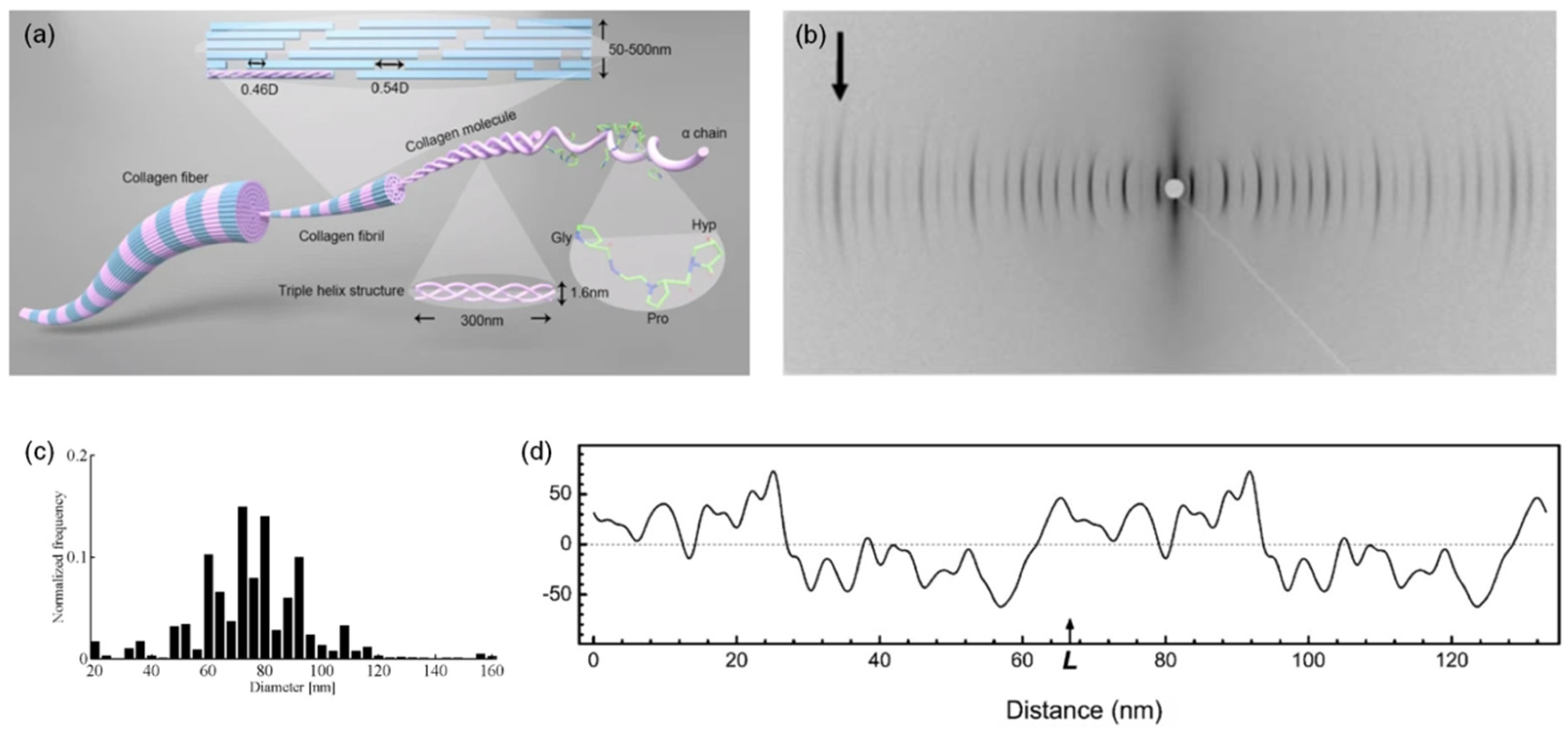
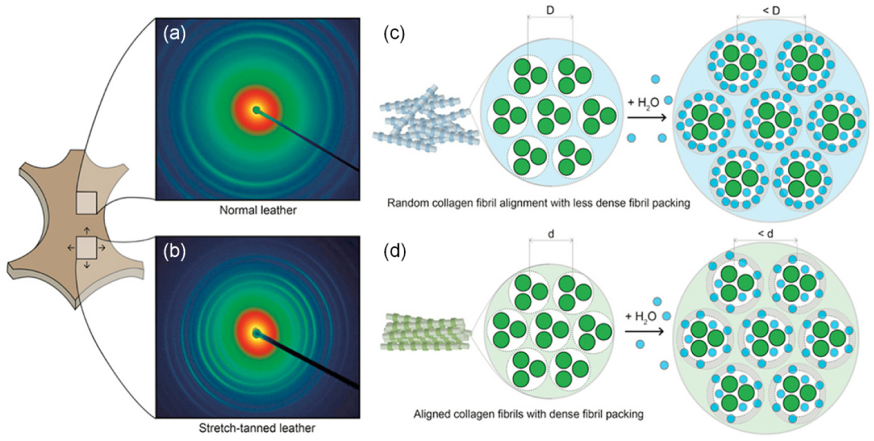
3.1. Collagen
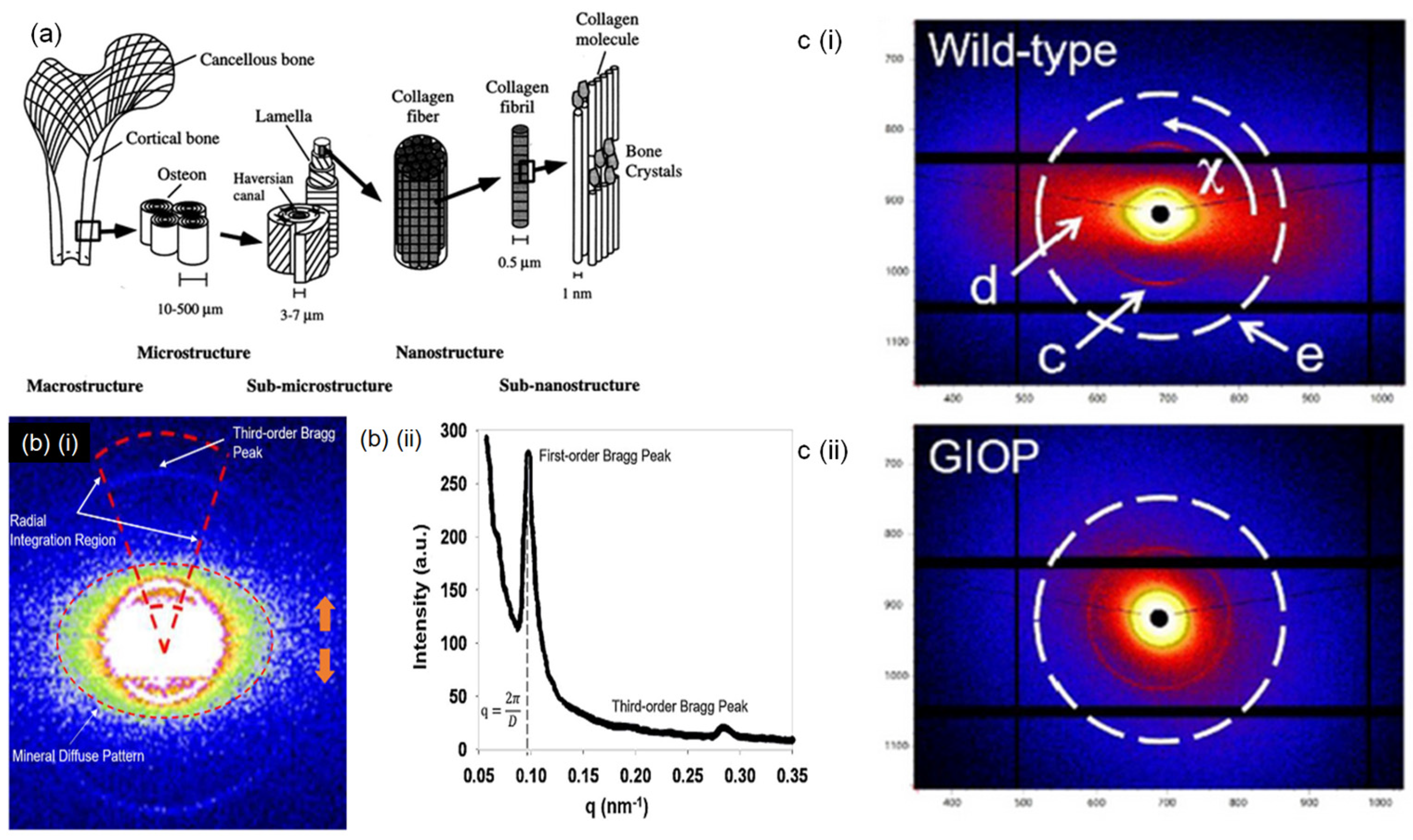
3.2. Bone
3.3. Hair
3.4. Feather
3.5. Silk
4. Lamellar Structures
5. Solution Scattering
5.1. Intrinsically Disordered Proteins
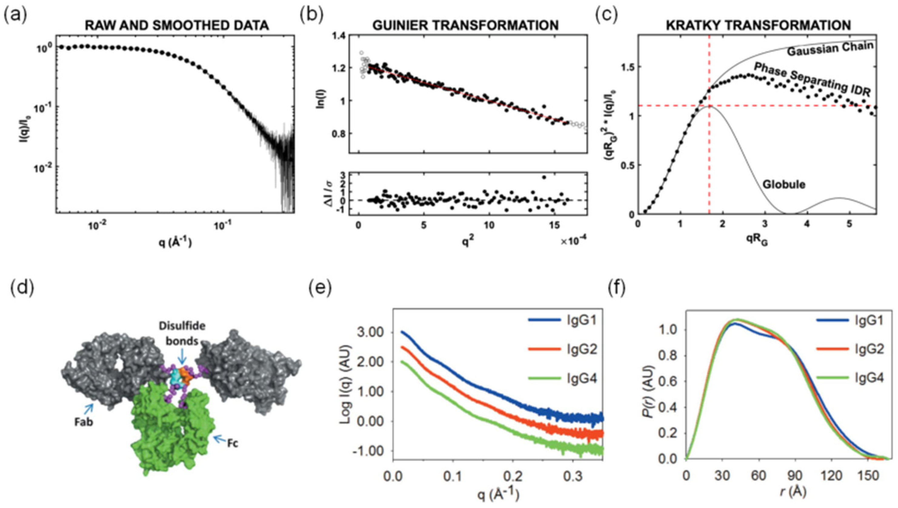
5.2. Multidomain Proteins
6. Conclusions
Author Contributions
Funding
Conflicts of Interest
References
- Imai, H. Self-Organized Formation of Hierarchical Structures. In Biomineralization I: Crystallization and Self-Organization Process; Naka, K., Ed.; Springer: Berlin/Heidelberg, Germany, 2007; pp. 43–72. [Google Scholar]
- Hedegaard, C.L.; Mata, A. Integrating self-assembly and biofabrication for the development of structures with enhanced complexity and hierarchical control. Biofabrication 2020, 12, 032002. [Google Scholar] [CrossRef] [PubMed]
- Murthy, N.S. X-ray Diffraction from Polymers. Polymer Morphology: Principles, Characterization, and Processing; John Wiley & Sons: Hoboken, NJ, USA, 2016; pp. 14–36. [Google Scholar]
- Müller, M.; Krasnov, I.; Ogurreck, M.; Blankenburg, M.; Pazera, T.; Seydel, T. Wood and Silk: Hierarchically Structured Biomaterials Investigated In Situ With X-Ray and Neutron Scattering. Adv. Eng. Mater. 2011, 13, 767–772. [Google Scholar] [CrossRef]
- Huang, W.; Restrepo, D.; Jung, J.Y.; Su, F.Y.; Liu, Z.; Ritchie, R.O.; McKittrick, J.; Zavattieri, P.; Kisailus, D. Multiscale toughening mechanisms in biological materials and bioinspired designs. Adv. Mater. 2019, 31, 1901561. [Google Scholar] [CrossRef] [PubMed]
- Wittig, N.K.; Birkedal, H. Bone hierarchical structure: Spatial variation across length scales. Acta Crystallogr. Sect. B Struct. Sci. Cryst. Eng. Mater. 2022, 78, 305–311. [Google Scholar] [CrossRef]
- Fratzl, P. Hierarchical structure and mechanical adaptation of biological materials. In Learning from Nature How to Design New Implantable Biomaterialsis: From Biomineralization Fundamentals to Biomimetic Materials and Processing Routes: Proceedings of the NATO Advanced Study Institute, held in Alvor, Algarve, Portugal, 13–24 October 2003; Springer: Dordrecht, The Netherlands, 2004; pp. 15–34. [Google Scholar]
- Paris, O. From diffraction to imaging: New avenues in studying hierarchical biological tissues with X-ray microbeams. Biointerphases 2008, 3, FB16–FB26. [Google Scholar] [CrossRef]
- Gautieri, A.; Vesentini, S.; Redaelli, A.; Buehler, M.J. Hierarchical structure and nanomechanics of collagen microfibrils from the atomistic scale up. Nano Lett. 2011, 11, 757–766. [Google Scholar] [CrossRef]
- Bish, D.L.; Reynolds, R.; Post, J. Sample preparation for X-ray diffraction. Mod. Powder Diffr. 1989, 20, 73–99. [Google Scholar]
- Riekel, C.; Vollrath, F. Spider silk fibre extrusion: Combined wide-and small-angle X-ray microdiffraction experiments. Int. J. Biol. Macromol. 2001, 29, 203–210. [Google Scholar] [CrossRef]
- Müller, M.; Burghammer, M.; Riekel, C. Combined scanning microdiffraction and micro small-angle scattering at the microfocus beamline ID13 (ESRF). Nucl. Instrum. Methods Phys. Res. Sect. A Accel. Spectrometers Detect. Assoc. Equip. 2001, 467, 958–961. [Google Scholar] [CrossRef]
- Cedola, A.; Lagomarsino, S.; Komlev, V.; Rustichelli, F.; Mastrogiacomo, M.; Cancedda, R.; Milita, S.; Burghammer, M. High spatial resolution X-ray microdiffraction applied to biomaterial studies and archeometry. Spectrochim. Acta Part B At. Spectrosc. 2004, 59, 1557–1564. [Google Scholar] [CrossRef]
- Riekel, C.; Burghammer, M.; Rosenthal, M. Skin-core morphology in spider flagelliform silk. Appl. Phys. Lett. 2019, 115, 123702. [Google Scholar] [CrossRef]
- Murthy, N.; Grubb, D.; Zero, K. Structural implications of the elliptical form of small-angle reflections in oriented semicrystalline polymers. Macromolecules 2000, 33, 1012–1021. [Google Scholar] [CrossRef]
- Singh, H.S.Y. The SAXS Guide: Getting Acquainted with the Princioples, 5th ed.; Anton Paar GmbH: Graz, Austria, 2023; p. 188. [Google Scholar]
- Lombardo, D.; Calandra, P.; Kiselev, M.A. Structural characterization of biomaterials by means of small angle X-rays and neutron scattering (SAXS and SANS), and light scattering experiments. Molecules 2020, 25, 5624. [Google Scholar] [CrossRef] [PubMed]
- Hughes, M.D.; Cook, K.R.; Cussons, S.; Boroumand, A.; Tyler, A.I.; Head, D.; Brockwell, D.J.; Dougan, L. Capturing Dynamic Assembly of Nanoscale Proteins During Network Formation. Small 2025, 21, 2407090. [Google Scholar] [CrossRef]
- Hamley, I.W.; Castelletto, V. Small-angle scattering techniques for peptide and peptide hybrid nanostructures and peptide-based biomaterials. Adv. Colloid Interface Sci. 2023, 318, 102959. [Google Scholar] [CrossRef]
- Rodriguez-Palomo, A.; Østergaard, M.; Birkedal, H. Bone hierarchical structure: Heterogeneity and uniformity. Adv. Funct. Mater. 2024, 34, 2307026. [Google Scholar] [CrossRef]
- Schmid, S.Y.; Lachowski, K.; Chiang, H.T.; Pozzo, L.; De Yoreo, J.; Zhang, S. Mechanisms of Biomolecular Self-Assembly Investigated Through In Situ Observations of Structures and Dynamics. Angew. Chem. Int. Ed. 2023, 62, e202309725. [Google Scholar] [CrossRef]
- Chen, D.; Ilavsky, J. Structural characterization of high-protein system through ultra-small and small-angle X-ray scattering (USAXS/SAXS). Curr. Opin. Food Sci. 2024, 59, 101204. [Google Scholar] [CrossRef]
- Du, Z.; Xu, N.; Yang, Y.; Li, G.; Tai, Z.; Li, N.; Sun, Y. Study on internal structure of casein micelles in reconstituted skim milk powder. Int. J. Biol. Macromol. 2023, 224, 437–452. [Google Scholar] [CrossRef]
- Raghuwanshi, V.S.; Mendoza, D.J.; Mata, J.; Garnier, G. Modulating the isotopic hydrogen-deuterium exchange in functionalized nanocellulose to optimize SANS contrast. Carbohydr. Polym. 2024, 345, 122591. [Google Scholar] [CrossRef]
- Liu, D.; Song, K.; Chen, W.; Chen, J.; Sun, G.; Li, L. Current progresses of small-angle neutron scattering on soft-matters investigation. Nucl. Anal. 2022, 1, 100011. [Google Scholar] [CrossRef]
- Brosey, C.A.; Tainer, J.A. Evolving SAXS versatility: Solution X-ray scattering for macromolecular architecture, functional landscapes, and integrative structural biology. Curr. Opin. Struct. Biol. 2019, 58, 197–213. [Google Scholar] [CrossRef] [PubMed]
- Feigin, L.; Svergun, D.I. Structure Analysis by Small-Angle X-Ray and Neutron Scattering; Springer: Berlin/Heidelberg, Germany, 1987; Volume 1. [Google Scholar]
- Kikhney, A.G.; Svergun, D.I. A practical guide to small angle X-ray scattering (SAXS) of flexible and intrinsically disordered proteins. FEBS Lett. 2015, 589, 2570–2577. [Google Scholar] [CrossRef] [PubMed]
- Koch, M.H.; Vachette, P.; Svergun, D.I. Small-angle scattering: A view on the properties, structures and structural changes of biological macromolecules in solution. Q. Rev. Biophys. 2003, 36, 147–227. [Google Scholar] [CrossRef]
- Meisburger, S.P.; Thomas, W.C.; Watkins, M.B.; Ando, N. X-ray scattering studies of protein structural dynamics. Chem. Rev. 2017, 117, 7615–7672. [Google Scholar] [CrossRef]
- Bear, R.S. X-ray diffraction studies on protein fibers. I. The large fiber-axis period of collagen. J. Am. Chem. Soc. 1944, 66, 1297–1305. [Google Scholar] [CrossRef]
- Feughelman, M. A two-phase structure for keratin fibers. Text. Res. J. 1959, 29, 223–228. [Google Scholar] [CrossRef]
- Murthy, N.; Wood, D.; Moscarello, M. X-ray scattering studies of a model complex of lipid and basic protein of myelin. Biochim. Biophys. Acta-Biomembr. 1984, 769, 493–498. [Google Scholar] [CrossRef]
- Murthy, N.S.; Worthington, C. X-ray diffraction analysis of dehydrated myelin. Biochim. Biophys. Acta-Biomembr. 1982, 689, 451–456. [Google Scholar] [CrossRef]
- Yang, Z.; Grubb, D.; Jelinski, L. Small-angle X-ray scattering of spider dragline silk. Macromolecules 1997, 30, 8254–8261. [Google Scholar] [CrossRef]
- Saranathan, V.; Narayanan, S.; Sandy, A.; Dufresne, E.R.; Prum, R.O. Evolution of single gyroid photonic crystals in bird feathers. Proc. Natl. Acad. Sci. USA 2021, 118, e2101357118. [Google Scholar] [CrossRef] [PubMed]
- Lakes, R. Materials with structural hierarchy. Nature 1993, 361, 511–515. [Google Scholar] [CrossRef]
- Murthy, N.S.; Wang, W.; Kamath, Y. Structure of intermediate filament assembly in hair deduced from hydration studies using small-angle neutron scattering. J. Struct. Biol. 2019, 206, 295–304. [Google Scholar] [CrossRef] [PubMed]
- Das, A.; Bahadur, J.; Kumar, A.; Sen, D. Performance of small-and wide-angle x-ray scattering beamline at Indus-2 synchrotron. Rev. Sci. Instrum. 2023, 94, 043902. [Google Scholar] [CrossRef]
- Noh, H.; Liew, S.F.; Saranathan, V.; Mochrie, S.G.; Prum, R.O.; Dufresne, E.R.; Cao, H. How noniridescent colors are generated by quasi-ordered structures of bird feathers. Adv. Mater. 2010, 22, 2871–2880. [Google Scholar] [CrossRef]
- Guinier, A. X-Ray Diffraction: In Crystals, Imperfect Crystals, and Amorphous Bodies; Freeman and Co.: Hong Kong, China, 1963. [Google Scholar]
- Guinier, A.; Fournet, G. Small Angle X-Ray Scattering; John Wiley & Sons, Inc.: New York, NY, USA, 1955. [Google Scholar]
- Putnam, C.D.; Hammel, M.; Hura, G.L.; Tainer, J.A. X-ray solution scattering (SAXS) combined with crystallography and computation: Defining accurate macromolecular structures, conformations and assemblies in solution. Q. Rev. Biophys. 2007, 40, 191–285. [Google Scholar] [CrossRef]
- Jacques, D.A.; Trewhella, J. Small-angle scattering for structural biology—Expanding the frontier while avoiding the pitfalls. Protein Sci. 2010, 19, 642–657. [Google Scholar] [CrossRef]
- Zhou, H.-X.; Bilsel, O. SAXS/SANS probe of intermolecular interactions in concentrated protein solutions. Biophys. J. 2014, 106, 771–773. [Google Scholar] [CrossRef]
- Kachala, M.; Valentini, E.; Svergun, D.I. Application of SAXS for the Structural Characterization of IDPs. Intrinsically Disord. Proteins Stud. By NMR Spectrosc. 2015, 870, 261–289. [Google Scholar]
- Graewert, M.A.; Svergun, D.I. Advanced sample environments and sample requirements for biological SAXS. In Methods in Enzymology; Elsevier: Amsterdam, The Netherlands, 2022; Volume 677, pp. 1–39. [Google Scholar]
- Garman, E.F.; Weik, M. X-ray radiation damage to biological samples: Recent progress. Synchrotron Radiat. 2019, 26, 907–911. [Google Scholar] [CrossRef]
- Stachowski, T.R.; Snell, M.E.; Snell, E.H. SAXS studies of X-ray induced disulfide bond damage: Engineering high-resolution insight from a low-resolution technique. PLoS ONE 2020, 15, e0239702. [Google Scholar] [CrossRef] [PubMed]
- Meisburger, S.P.; Warkentin, M.; Chen, H.; Hopkins, J.B.; Gillilan, R.E.; Pollack, L.; Thorne, R.E. Breaking the radiation damage limit with cryo-SAXS. Biophys. J. 2013, 104, 227–236. [Google Scholar] [CrossRef] [PubMed]
- Schneidman-Duhovny, D.; Hammel, M.; Tainer, J.A.; Sali, A. Accurate SAXS profile computation and its assessment by contrast variation experiments. Biophys. J. 2013, 105, 962–974. [Google Scholar] [CrossRef] [PubMed]
- Karamanos, N.K.; Theocharis, A.D.; Piperigkou, Z.; Manou, D.; Passi, A.; Skandalis, S.S.; Vynios, D.H.; Orian-Rousseau, V.; Ricard-Blum, S.; Schmelzer, C.E. A guide to the composition and functions of the extracellular matrix. FEBS J. 2021, 288, 6850–6912. [Google Scholar] [CrossRef]
- Glimcher, M.J. Bone: Nature of the calcium phosphate crystals and cellular, structural, and physical chemical mechanisms in their formation. Rev. Mineral. Geochem. 2006, 64, 223–282. [Google Scholar] [CrossRef]
- Weiner, S.; Wagner, H.D. The material bone: Structure-mechanical function relations. Annu. Rev. Mater. Sci. 1998, 28, 271–298. [Google Scholar] [CrossRef]
- Briki, F.; Busson, B.; Doucet, J. Organization of microfibrils in keratin fibers studied by X-ray scattering: Modelling using the paracrystal concept. Biochim. Biophys. Acta Protein Struct. Mol. Enzymol. 1998, 1429, 57–68. [Google Scholar] [CrossRef]
- Piccinini, A.; Lucia, G.; Colarossi, D.; Principi, P.; Amenitsch, H.; Regoli, F.; Gorbi, S.; Spinozzi, F. Microfibers Degradation Processes in Water Under Simulated Solar Irradiation: A Small-and Wide-Angle X-Ray Scattering Study. Available online: https://papers.ssrn.com/sol3/papers.cfm?abstract_id=4587585 (accessed on 10 April 2025).
- Rafik, M.E.; Doucet, J.; Briki, F. The intermediate filament architecture as determined by X-ray diffraction modeling of hard α-keratin. Biophys. J. 2004, 86, 3893–3904. [Google Scholar] [CrossRef]
- Keten, S.; Xu, Z.; Ihle, B.; Buehler, M.J. Nanoconfinement controls stiffness, strength and mechanical toughness of β-sheet crystals in silk. Nat. Mater. 2010, 9, 359–367. [Google Scholar] [CrossRef]
- Ottani, V.; Martini, D.; Franchi, M.; Ruggeri, A.; Raspanti, M. Hierarchical structures in fibrillar collagens. Micron 2002, 33, 587–596. [Google Scholar] [CrossRef]
- Chen, Q.; Pei, Y.; Tang, K.; Albu-Kaya, M.G. Structure, extraction, processing, and applications of collagen as an ideal component for biomaterials—A review. Collagen Leather 2023, 5, 20. [Google Scholar] [CrossRef]
- Burger, C.; Zhou, H.w.; Sicŝ, I.; Hsiao, B.S.; Chu, B.; Graham, L.; Glimcher, M.J. Small-angle X-ray scattering study of intramuscular fish bone: Collagen fibril superstructure determined from equidistant meridional reflections. J. Appl. Crystallogr. 2008, 41, 252–261. [Google Scholar] [CrossRef]
- Goh, K.L.; Hiller, J.; Haston, J.L.; Holmes, D.F.; Kadler, K.E.; Murdoch, A.; Meakin, J.R.; Wess, T.J. Analysis of collagen fibril diameter distribution in connective tissues using small-angle X-ray scattering. Biochim. Et Biophys. Acta-Gen. Subj. 2005, 1722, 183–188. [Google Scholar] [CrossRef]
- Kelly, S.; Weinkamer, R.; Bertinetti, L.; Edmonds, R.; Sizeland, K.; Wells, H.; Fratzl, P.; Haverkamp, R. Effect of collagen packing and moisture content on leather stiffness. J. Mech. Behav. Biomed. Mater. 2019, 90, 1–10. [Google Scholar] [CrossRef]
- Suhonen, H.; Fernández, M.; Serimaa, R.; Suortti, P. Simulation of small-angle X-ray scattering from collagen fibrils and comparison with experimental patterns. Phys. Med. Biol. 2005, 50, 5401. [Google Scholar] [CrossRef]
- Haverkamp, R.G.; Sizeland, K.H.; Wells, H.C.; Kamma-Lorger, C. Collagen dehydration. Int. J. Biol. Macromol. 2022, 216, 140–147. [Google Scholar] [CrossRef]
- Zhang, Y.; Buchanan, J.; Naffa, R.; Mansel, B.; Maidment, C.; Holmes, G.; Prabakar, S. In situ structural studies during denaturation of natural and synthetically crosslinked collagen using synchrotron SAXS. Synchrotron Radiat. 2020, 27, 1376–1381. [Google Scholar] [CrossRef]
- Zhang, Y.; Ingham, B.; Leveneur, J.; Cheong, S.; Yao, Y.; Clarke, D.J.; Holmes, G.; Kennedy, J.; Prabakar, S. Can sodium silicates affect collagen structure during tanning? Insights from small angle X-ray scattering (SAXS) studies. RSC Adv. 2017, 7, 11665–11671. [Google Scholar] [CrossRef]
- Acerbo, A.S.; Kwaczala, A.T.; Yang, L.; Judex, S.; Miller, L.M. Alterations in collagen and mineral nanostructure observed in osteoporosis and pharmaceutical treatments using simultaneous small-and wide-angle X-ray scattering. Calcif. Tissue Int. 2014, 95, 446–456. [Google Scholar] [CrossRef]
- Moger, C.; Barrett, R.; Bleuet, P.; Bradley, D.; Ellis, R.; Green, E.; Knapp, K.; Muthuvelu, P.; Winlove, C. Regional variations of collagen orientation in normal and diseased articular cartilage and subchondral bone determined using small angle X-ray scattering (SAXS). Osteoarthr. Cartil. 2007, 15, 682–687. [Google Scholar] [CrossRef]
- Meek, K.M.; Boote, C. The use of X-ray scattering techniques to quantify the orientation and distribution of collagen in the corneal stroma. Prog. Retin. Eye Res. 2009, 28, 369–392. [Google Scholar] [CrossRef] [PubMed]
- Bell, J.; Hayes, S.; Whitford, C.; Sanchez-Weatherby, J.; Shebanova, O.; Vergari, C.; Winlove, C.; Terrill, N.; Sorensen, T.; Elsheikh, A. The hierarchical response of human corneal collagen to load. Acta Biomater. 2018, 65, 216–225. [Google Scholar] [CrossRef]
- Liu, Y.; Luo, D.; Wang, T. Hierarchical structures of bone and bioinspired bone tissue engineering. Small 2016, 12, 4611–4632. [Google Scholar] [CrossRef]
- Singhal, A. Study of Mechanical Properties of Bone by Measuring Load Transfer via High-Energy X-Ray Diffraction. Doctoral Dissertation, Northwestern University, Evanston, IL, USA, 2012. [Google Scholar]
- Rho, J.-Y.; Kuhn-Spearing, L.; Zioupos, P. Mechanical properties and the hierarchical structure of bone. Med. Eng. Phys. 1998, 20, 92–102. [Google Scholar] [CrossRef]
- Ma, S.; Boughton, O.; Karunaratne, A.; Jin, A.; Cobb, J.; Hansen, U.; Abel, R. Synchrotron imaging assessment of bone quality. Clin. Rev. Bone Miner. Metab. 2016, 14, 150–160. [Google Scholar] [CrossRef]
- Xi, L.; Zhang, Y.; Gupta, H.; Terrill, N.; Wang, P.; Zhao, T.; Fang, D. A multiscale study of structural and compositional changes in a natural nanocomposite: Osteoporotic bone with chronic endogenous steroid excess. Bone 2021, 143, 115666. [Google Scholar] [CrossRef]
- Pabisch, S.; Wagermaier, W.; Zander, T.; Li, C.; Fratzl, P. Imaging the nanostructure of bone and dentin through small-and wide-angle X-ray scattering. Methods Enzymol. 2013, 532, 391–413. [Google Scholar]
- Zimmermann, E.A.; Schaible, E.; Gludovatz, B.; Schmidt, F.N.; Riedel, C.; Krause, M.; Vettorazzi, E.; Acevedo, C.; Hahn, M.; Püschel, K. Intrinsic mechanical behavior of femoral cortical bone in young, osteoporotic and bisphosphonate-treated individuals in low-and high energy fracture conditions. Sci. Rep. 2016, 6, 21072. [Google Scholar] [CrossRef]
- Popescu, C.; Höcker, H. Hair—The most sophisticated biological composite material. Chem. Soc. Rev. 2007, 36, 1282–1291. [Google Scholar] [CrossRef]
- Stanić, V.; Bettini, J.; Montoro, F.E.; Stein, A.; Evans-Lutterodt, K. Local structure of human hair spatially resolved by sub-micron X-ray beam. Sci. Rep. 2015, 5, 17347. [Google Scholar] [CrossRef]
- Harland, D.P.; Walls, R.J.; Vernon, J.A.; Dyer, J.M.; Woods, J.L.; Bell, F. Three-dimensional architecture of macrofibrils in the human scalp hair cortex. J. Struct. Biol. 2014, 185, 397–404. [Google Scholar] [CrossRef] [PubMed]
- Yu, Y.; Yang, W.; Wang, B.; Meyers, M.A. Structure and mechanical behavior of human hair. Mater. Sci. Eng. C 2017, 73, 152–163. [Google Scholar] [CrossRef]
- Greenberg, D.A.; Fudge, D.S. Regulation of hard α-keratin mechanics via control of intermediate filament hydration: Matrix squeeze revisited. Proc. R. Soc. B Biol. Sci. 2013, 280, 20122158. [Google Scholar] [CrossRef]
- Kreplak, L.; Doucet, J.; Briki, F. Unraveling double stranded α-helical coiled coils: An x-ray diffraction study on hard α-keratin fibers. Biopolym. Orig. Res. Biomol. 2001, 58, 526–533. [Google Scholar] [CrossRef]
- Kreplak, L.; Mérigoux, C.; Briki, F.; Flot, D.; Doucet, J. Investigation of human hair cuticle structure by microdiffraction: Direct observation of cell membrane complex swelling. Biochim. Biophys. Acta-Protein Struct. Mol. Enzymol. 2001, 1547, 268–274. [Google Scholar] [CrossRef]
- Wade, M.; Tucker, I.; Cunningham, P.; Skinner, R.; Bell, F.; Lyons, T.; Patten, K.; Gonzalez, L.; Wess, T. Investigating the origins of nanostructural variations in differential ethnic hair types using X-ray scattering techniques. Int. J. Cosmet. Sci. 2013, 35, 430–441. [Google Scholar] [CrossRef]
- Lima, C.; Lima, R.; Bandeira, A.; Couto, R.; Velasco, M.; Bordallo, H.N.; Oliveira, C. Alterations promoted by acid straightening and/or bleaching in hair microstructures. Appl. Crystallogr. 2023, 56, 1002–1014. [Google Scholar] [CrossRef]
- Lima, C.R.R.d.C.; Lima, R.; Machado, L.; Velasco, M.V.R.; Lakic, L.; Nordentoft, M.; Machuca-Beier, L.; Rudić, S.; Telling, M.; Sakai, V.G. Human hair: Subtle change in the thioester groups dynamics observed by combining neutron scattering, X-ray diffraction and thermal analysis. Eur. Phys. J. Spec. Top. 2020, 229, 2825–2832. [Google Scholar] [CrossRef]
- Terrill, R.S.; Shultz, A.J. Feather function and the evolution of birds. Biol. Rev. 2023, 98, 540–566. [Google Scholar] [CrossRef]
- Janas, K.; Łatkiewicz, A.; Parnell, A.; Lutyk, D.; Barczyk, J.; Shawkey, M.D.; Gustafsson, L.; Cichoń, M.; Drobniak, S.M. Differential effects of early growth conditions on colour-producing nanostructures revealed through small angle X-ray scattering and electron microscopy. J. Exp. Biol. 2020, 223, jeb228387. [Google Scholar] [CrossRef]
- Saranathan, V.; Forster, J.D.; Noh, H.; Liew, S.-F.; Mochrie, S.G.; Cao, H.; Dufresne, E.R.; Prum, R.O. Structure and optical function of amorphous photonic nanostructures from avian feather barbs: A comparative small angle X-ray scattering (SAXS) analysis of 230 bird species. J. R. Soc. Interface 2012, 9, 2563–2580. [Google Scholar] [CrossRef]
- Noh, H.; Liew, S.F.; Saranathan, V.; Prum, R.O.; Mochrie, S.G.; Dufresne, E.R.; Cao, H. Contribution of double scattering to structural coloration in quasiordered nanostructures of bird feathers. Phys. Rev. E—Stat. Nonlinear Soft Matter Phys. 2010, 81, 051923. [Google Scholar] [CrossRef]
- Prum, R.O.; Dufresne, E.R.; Quinn, T.; Waters, K. Development of colour-producing β-keratin nanostructures in avian feather barbs. J. R. Soc. Interface 2009, 6 (Suppl. 2), S253–S265. [Google Scholar] [CrossRef]
- Wang, Q.; Ling, S.; Yao, Q.; Li, Q.; Hu, D.; Dai, Q.; Weitz, D.A.; Kaplan, D.L.; Buehler, M.J.; Zhang, Y. Observations of 3 nm silk nanofibrils exfoliated from natural silkworm silk fibers. ACS Mater. Lett. 2020, 2, 153–160. [Google Scholar] [CrossRef]
- Yoshioka, T.; Kameda, T.; Burghammer, M.; Riekel, C. Mesoscale confinement in Bagworm silk: A hidden structural organization. Nano Lett. 2023, 23, 827–834. [Google Scholar] [CrossRef]
- Wang, W.; Murthy, N.S.; Grubb, D.T. Central small-angle diffuse scattering from fibers is made of two components. J. Polym. Sci. Part B Polym. Phys. 2012, 50, 797–804. [Google Scholar] [CrossRef]
- Yoshioka, T.; Kameda, T. X-ray scattering analyses quantitatively revealed periodic hierarchical structure of polyalanine β-sheet and non-polyalanine amorphous domains in Antheraea assamensis (Muga) silk. J. Silk Sci. Technol. Jpn. 2019, 27, 95–101. [Google Scholar]
- Yoshioka, T.; Kameda, T. Hexagonal packing of nanofibrils in Bombyx mori silkworm silk revealed by small-angle X-ray scattering analysis. J. Silk Sci. Technol. Jpn. 2020, 28, 127–133. [Google Scholar]
- Yoshioka, T.; Tsubota, T.; Tashiro, K.; Jouraku, A.; Kameda, T. A study of the extraordinarily strong and tough silk produced by bagworms. Nat. Commun. 2019, 10, 1469. [Google Scholar] [CrossRef]
- Prum, R.O. Evolution of the morphological innovations of feathers. J. Exp. Zool. Part B Mol. Dev. Evol. 2005, 304, 570–579. [Google Scholar] [CrossRef]
- Reznikov, N.; Shahar, R.; Weiner, S. Bone hierarchical structure in three dimensions. Acta Biomater. 2014, 10, 3815–3826. [Google Scholar] [CrossRef]
- Sun, J.; Bhushan, B. Hierarchical structure and mechanical properties of nacre: A review. Rsc Adv. 2012, 2, 7617–7632. [Google Scholar] [CrossRef]
- Li, X.-W.; Ji, H.-M.; Yang, W.; Zhang, G.-P.; Chen, D.-L. Mechanical properties of crossed-lamellar structures in biological shells: A review. J. Mech. Behav. Biomed. Mater. 2017, 74, 54–71. [Google Scholar] [CrossRef]
- Murthy, N.S.; Kennedy, W.; Koerner, H.; Grubb, D. Small-Angle X-ray Scattering from Lamellar Structures. Polymer 2021, 220, 123566. [Google Scholar]
- Blanco-González, A.; Piñeiro, Á.; García-Fandiño, R. Unravelling hierarchical levels of structure in lipid membranes. Comput. Struct. Biotechnol. J. 2022, 20, 2798–2806. [Google Scholar] [CrossRef]
- Simidjiev, I.; Stoylova, S.; Amenitsch, H.; Jávorfi, T.; Mustárdy, L.; Laggner, P.; Holzenburg, A.; Garab, G. Self-assembly of large, ordered lamellae from non-bilayer lipids and integral membrane proteins in vitro. Proc. Natl. Acad. Sci. USA 2000, 97, 1473–1476. [Google Scholar] [CrossRef]
- Pasteris, J.D.; Wopenka, B.; Valsami-Jones, E. Bone and tooth mineralization: Why apatite? Elements 2008, 4, 97–104. [Google Scholar] [CrossRef]
- Kiselev, M.A.; Lombardo, D. Structural characterization in mixed lipid membrane systems by neutron and X-ray scattering. Biochim. Biophys. Acta-Gen. Subj. 2017, 1861, 3700–3717. [Google Scholar] [CrossRef]
- Stadelmann, C.; Timmler, S.; Barrantes-Freer, A.; Simons, M. Myelin in the central nervous system: Structure, function, and pathology. Physiol. Rev. 2019, 99, 1381–1431. [Google Scholar] [CrossRef]
- Perrelle, J.M.; Boreland, A.J.; Gamboa, J.M.; Gowda, P.; Murthy, N.S. Biomimetic strategies for peripheral nerve injury repair: An exploration of microarchitecture and cellularization. Biomed. Mater. Devices 2023, 1, 21–37. [Google Scholar] [CrossRef]
- Pabst, G.; Rappolt, M.; Amenitsch, H.; Laggner, P. Structural information from multilamellar liposomes at full hydration: Full q-range fitting with high quality x-ray data. Phys. Rev. E 2000, 62, 4000. [Google Scholar] [CrossRef] [PubMed]
- Hamley, I.W. Diffuse scattering from lamellar structures. Soft Matter 2022, 18, 711–721. [Google Scholar] [CrossRef]
- De Felici, M.; Felici, R.; Ferrero, C.; Tartari, A.; Gambaccini, M.; Finet, S. Structural characterization of the human cerebral myelin sheath by small angle x-ray scattering. Phys. Med. Biol. 2008, 53, 5675. [Google Scholar] [CrossRef]
- Georgiadis, M.; Schroeter, A.; Gao, Z.; Guizar-Sicairos, M.; Liebi, M.; Leuze, C.; McNab, J.A.; Balolia, A.; Veraart, J.; Ades-Aron, B. Nanostructure-specific X-ray tomography reveals myelin levels, integrity and axon orientations in mouse and human nervous tissue. Nat. Commun. 2021, 12, 2941. [Google Scholar] [CrossRef]
- Baroni, D.; Zegarra-Moran, O.; Moran, O. Functional and pharmacological induced structural changes of the cystic fibrosis transmembrane conductance regulator in the membrane solved using SAXS. Cell. Mol. Life Sci. 2015, 72, 1363–1375. [Google Scholar] [CrossRef]
- Carrotta, R.; Mangione, M.R.; Librizzi, F.; Moran, O. Small angle X-ray scattering sensing membrane composition: The role of sphingolipids in membrane-amyloid β-peptide interaction. Biology 2021, 11, 26. [Google Scholar] [CrossRef]
- Ciesiołkiewicz, A.; Perez, J.L.; Berlicki, Ł. Miniproteins in medicinal chemistry. Bioorgan. Med. Chem. Lett. 2022, 71, 128806. [Google Scholar] [CrossRef]
- Clarke, N.D.; Ezkurdia, I.; Kopp, J.; Read, R.J.; Schwede, T.; Tress, M. Domain definition and target classification for CASP7. Proteins: Struct. Funct. Bioinform. 2007, 69, 10–18. [Google Scholar] [CrossRef]
- Vazquez, D.S.; Toledo, P.L.; Gianotti, A.R.; Ermácora, M.R. Protein conformation and biomolecular condensates. Curr. Res. Struct. Biol. 2022, 4, 285–307. [Google Scholar] [CrossRef]
- Receveur-Bréchot, V.; Durand, D. How random are intrinsically disordered proteins? A small angle scattering perspective. Curr. Protein Pept. Sci. 2012, 13, 55–75. [Google Scholar] [CrossRef]
- Sibille, N.; Bernado, P. Structural characterization of intrinsically disordered proteins by the combined use of NMR and SAXS. Biochem. Soc. Trans. 2012, 40, 955–962. [Google Scholar] [CrossRef] [PubMed]
- Durand, D.; Vivès, C.; Cannella, D.; Pérez, J.; Pebay-Peyroula, E.; Vachette, P.; Fieschi, F. NADPH oxidase activator p67phox behaves in solution as a multidomain protein with semi-flexible linkers. J. Struct. Biol. 2010, 169, 45–53. [Google Scholar] [CrossRef]
- Martin, E.W.; Hopkins, J.B.; Mittag, T. Small-angle X-ray scattering experiments of monodisperse intrinsically disordered protein samples close to the solubility limit. In Methods in Enzymology; Elsevier: Amsterdam, The Netherlands, 2021; Volume 646, pp. 185–222. [Google Scholar]
- Tian, X.; Vestergaard, B.; Thorolfsson, M.; Yang, Z.; Rasmussen, H.B.; Langkilde, A.E. In-depth analysis of subclass-specific conformational preferences of IgG antibodies. IUCrJ 2015, 2, 9–18. [Google Scholar] [CrossRef]
- Johansen, D.; Trewhella, J.; Goldenberg, D.P. Fractal dimension of an intrinsically disordered protein: Small-angle X-ray scattering and computational study of the bacteriophage λ N protein. Protein Sci. 2011, 20, 1955–1970. [Google Scholar] [CrossRef]
- Svergun, D.I. Restoring low resolution structure of biological macromolecules from solution scattering using simulated annealing. Biophys. J. 1999, 76, 2879–2886. [Google Scholar] [CrossRef]
- Lilyestrom, W.G.; Yadav, S.; Shire, S.J.; Scherer, T.M. Monoclonal antibody self-association, cluster formation, and rheology at high concentrations. J. Phys. Chem. B 2013, 117, 6373–6384. [Google Scholar] [CrossRef]
- Dear, B.J.; Bollinger, J.A.; Chowdhury, A.; Hung, J.J.; Wilks, L.R.; Karouta, C.A.; Ramachandran, K.; Shay, T.Y.; Nieto, M.P.; Sharma, A. X-ray scattering and coarse-grained simulations for clustering and interactions of monoclonal antibodies at high concentrations. J. Phys. Chem. B 2019, 123, 5274–5290. [Google Scholar] [CrossRef]
- Bayer, V. An overview of monoclonal antibodies. In Seminars in Oncology Nursing; Elsevier: Amsterdam, The Netherlands, 2019; p. 150927. [Google Scholar]
- Mahapatra, S.; Polimeni, M.; Gentiluomo, L.; Roessner, D.; Frieß, W.; Peters, G.N.H.; Streicher, W.W.; Lund, M.; Harris, P. Self-interactions of two monoclonal antibodies: Small-angle X-ray scattering, light scattering, and coarse-grained modeling. Mol. Pharm. 2021, 19, 508–519. [Google Scholar] [CrossRef]
- Larpent, P.; Codan, L.; Bothe, J.R.; Iuzzolino, L.; Pabit, S.; Gupta, S.; Fischmann, T.; Su, Y.; Reichert, P.; Stueber, D. Small-Angle X-ray Scattering as a Powerful Tool for Phase and Crystallinity Assessment of Monoclonal Antibody Crystallites in Support of Batch Crystallization. Mol. Pharm. 2024, 21, 4024–4037. [Google Scholar] [CrossRef]
- Wang, T.; Chen, J.; Du, X.; Feng, G.; Dai, T.; Li, X.; Liu, D. How neutron scattering techniques benefit investigating structures and dynamics of monoclonal antibody. Biochim. Biophys. Acta-Gen. Subj. 2022, 1866, 130206. [Google Scholar] [CrossRef]


Disclaimer/Publisher’s Note: The statements, opinions and data contained in all publications are solely those of the individual author(s) and contributor(s) and not of MDPI and/or the editor(s). MDPI and/or the editor(s) disclaim responsibility for any injury to people or property resulting from any ideas, methods, instructions or products referred to in the content. |
© 2025 by the authors. Licensee MDPI, Basel, Switzerland. This article is an open access article distributed under the terms and conditions of the Creative Commons Attribution (CC BY) license (https://creativecommons.org/licenses/by/4.0/).
Share and Cite
Patel, A.S.; Murthy, N.S. SAXS Investigation of Hierarchical Structures in Biological Materials. Appl. Sci. 2025, 15, 4472. https://doi.org/10.3390/app15084472
Patel AS, Murthy NS. SAXS Investigation of Hierarchical Structures in Biological Materials. Applied Sciences. 2025; 15(8):4472. https://doi.org/10.3390/app15084472
Chicago/Turabian StylePatel, Avi S., and N. Sanjeeva Murthy. 2025. "SAXS Investigation of Hierarchical Structures in Biological Materials" Applied Sciences 15, no. 8: 4472. https://doi.org/10.3390/app15084472
APA StylePatel, A. S., & Murthy, N. S. (2025). SAXS Investigation of Hierarchical Structures in Biological Materials. Applied Sciences, 15(8), 4472. https://doi.org/10.3390/app15084472