Deep Reinforcement Learning-Based Uncalibrated Visual Servoing Control of Manipulators with FOV Constraints

Abstract

In this article, we put forward a brand-new uncalibrated image-based visual servoing (IBVS) method. It is designed for monocular hand–eye manipulators with Field-of-View (FOV) feature constraints and makes use of a deep reinforcement learning (DRL) approach. First, the IBVS and its feature-loss problems are introduced. Then, a uncalibrated IBVS method is presented to address the feature-loss issue and improve servo efficiency with DRL. Specifically, the uncalibrated IBVS is integrated into the deep Q-network (DQN) control framework to ensure analytical stability. Additionally, a feature-constrained Q-network based on offline camera FOV environment feature mapping is designed and trained to adaptively output compensation for the IBVS controller, which helps maintain the feature within the camera’s FOV and improve servo performance. Finally, to further demonstrate the effectiveness and practicality of the proposed DQN-based uncalibrated IBVS method, experiments are conducted on a 6-DOF manipulator, and the results validate the proposed approach.

1. Introduction

Visual servoing control technology represents a closed-loop approach that makes use of vision feedback information [1]. The visual sensors empower the robot to explore its workspace with high reliability and execute intricate tasks within unstructured settings. Therefore, robots integrated with visual servoing control technology are also widely applied in the fields of automatic driving [2], automatic drilling [3], and robotic services [4,5].

In general, based on the different feedback information from the system, visual servoing can be categorized into position-based visual servoing (PBVS) [6,7], image-based visual servoing (IBVS) [8,9], and hybrid visual servoing (HVS) [10]. PBVS utilizes 2D image data to reconstruct the robot’s pose relative to the environmental objects. The accuracy of the pose information is highly sensitive to camera calibration errors. Compared with PBVS, since IBVS directly utilizes 2D image information to construct a closed-loop control, it eliminates the pose reconstruction step, making the control scheme more concise. In contrast, HVS combines the control mechanisms of both PBVS and IBVS. Due to the concise control scheme of IBVS and being less sensitive to camera calibration error, it has gained much attention in the visual servoing field. In [11], the IBVS method was used to achieve camera window tracking control for a quadrotor drone. The C-IBVS method introduced in [12] improves the convergence speed by incorporating a classical proportional controller, which exponentially reduces the tracking error. In [13], the convergence time was reduced by incorporating fuzzy logic techniques into the IBVS method. The Sliding Mode Control (SMC) method was used in [14] to cope with the problems of external perturbations and parameter uncertainties in the system, which has already enhanced the stability and robustness of the IBVS. In order to solve the IBVS problems with physical constraints, Model Predictive Control (MPC) methods were proposed in [15,16].

The above methods assumes that the target always remains within the camera’s FOV and that the features can be detected during the entire servo process. If the visibility constraint problem in IBVS is not considered, the continuous feedback link of feature information may be interrupted or become an outlier. In practical applications, due to the camera’s limited FOV, vision-based navigation [17], vision-based tracking and localization [18], etc., may all lead to issues of feature loss, which can lead to task interruptions and even cause unpredictable motion of the robot. Therefore, in practical vision servo applications, the FOV constraint of uncalibrated IBVS is an issue that needs to be considered.

To prevent feature loss, numerous approaches have been proposed in recent decades. For example, motion path planning methods are used to constrain visual features within the camera’s FOV. Wang et al. [19] presented a virtual target-guided RRT algorithm that iteratively explores a scaled Euclidean space under unknown image depth to identify paths that comply with FOV constraints. However, motion planning requires establishing a corresponding robot workspace model and is dependent on the accuracy of camera calibration [20]. Further, ref. [21,22] ensure FOV constraints by yet planning the camera’s Cartesian path. In [23], the potential function (PF) method is used to constrain features in the image danger zone within the safe region. In [24,25], the navigation function method is used to constrain image features within the camera’s FOV safe zone. But for the potential function and navigation function methods, the construction of the corresponding functions in the image plane requires careful design to be suitable for the specific IBVS tasks. A control barrier function-based method was proposed in [26] to constrain the maximum deviation between visual feature coordinates and the image plane center, ensuring that the features always remain within the FOV. In [27], the MPC method was proposed to optimize the feature trajectory in the image frame, addressing the field-of-view (FOV) constraint issue. In recent years, the rapid development of artificial intelligence has led to the widespread application of machine learning in the field of robotics. In [28], reinforcement learning (RL) is utilized to avoid feature loss in visual servoing tasks. In [29], to solve the feature visibility issue in the camera’s FOV for wheeled mobile robots (WMRs), a controller based on Q-learning is proposed to constrain visual features within the safe region of the image plane. To overcome the complexity of constructing a discretized Q-table in continuous environments, ref. [30] proposes the use of DQN to address this issue. However, these methods are only applicable to specific scenarios and have limited generalization capabilities. Compared to directly using RL as the output of the control system, [31,32] adopt Q-learning methods to adaptively adjust the IBVS servo gains and further propose a fuzzy control approach to adjust the RL learning rate, which not only ensures feature FOV visibility but also improves the servo convergence efficiency. In [33], a continuous action space design was adopted, utilizing the Deterministic Policy Gradient (DDPG) algorithm to adjust the gain of the IBVS controller. However, these parameter-based estimation methods do not take into account the specific feature FOV constraint issue.

Regarding the feature FOV constraint problem in IBVS, particularly in unknown noisy environments, the uncalibrated 6-DOF manipulator still faces challenges in handling multidimensional visual feature tasks, in order to ensure real-time performance and convergence efficiency. Therefore, to address the above issues, this paper proposes a DQN-based uncalibrated IBVS method. The main contributions of this paper are as follows:

(1)

A novel uncalibrated IBVS framework is proposed to address the feature constraint problem in the manipulator’s visual servoing task under unknown noise environments. The framework effectively mitigates the motion randomness caused by errors in the estimation of the feature–motion mapping matrix.

(2)

Base on DQN, the offline FOV feature mapping mechanism further is designed. Additionally, a camera FOV-based reward and punishment mechanism is established to train the visual feature agent to perform the uncalibrated visual servoing task with FOV constraints.

(3)

The new DQN-based uncalibrated visual servoing scheme achieves the auxiliary positioning task for 6-DOF manipulators, directly utilizing the feature states from 2D images to enforce visual feature constraints. This ensures the operational flexibility and stability of the uncalibrated visual servoing task in unknown noisy environments, making it more suitable for industrial robot applications.

Further, a comparison of our work with existing relevant work is provided in

Table 1. Comparison of existing relevant work.

Methods	Controlled Object	Main Contributions	FOV Constraint
[19]	Nonholonomic mobile robots	Combining the RRT algorithm with virtual goal-guided constraint planning increases the computational burden and may affect real-time performance.	√
[21,22]	6-DOF robot arm	In 3D space, trajectories that satisfy field-of-view constraints rely on accurate environment and system modeling.	√
[23]	6-DOF robot manipulator	The potential function approach may suffer from the problem of local minima, which may cause the control system to stagnate at a local optimum.	×
[26]	Quadrotor	The behavior of the system is constrained by the visible set, which is limited by a control barrier function.	√
[27]	6-DOF robot manipulator	Actuator limitations and visibility constraints can be addressed using the MPC strategy while considering computational complexity.	√
[29]	WMRs	The Q-learning controller was designed for the simple movements of wheeled robots.	×
[31,32]	Quadrotor	Designing adaptive servo gains with Q-learning can improve control without considering FOV.	×
[33]	WMRs	Designing adaptive servo gains with DDPG can improve control without considering FOV, and DDPG requires extensive data interactions and training, which can result in high computational cost and time overhead.	√
Ours	6-DOF robot manipulator	In the case where the system model is unknown and FOV feature constraints are considered, the DQN directly enforces the feature constraints using the mapped states of the camera FOV image features.	√

.

The structure of this paper is as follows: Section 2 discusses the nonlinear model of the IBVS manipulators. Section 3 presents the feature-constrained method based on DQN, further constructing and training the feature-constrained Q-network based on offline camera FOV environment feature mapping. Section 4 presents the DQN feature-constrained visual servoing framework. Section 5 demonstrates the proposed method through experiments conducted on a 6-DOF manipulator equipped with a hand–eye camera. Section 6 and Section 7 provide, respectively, the discussion and conclusions.

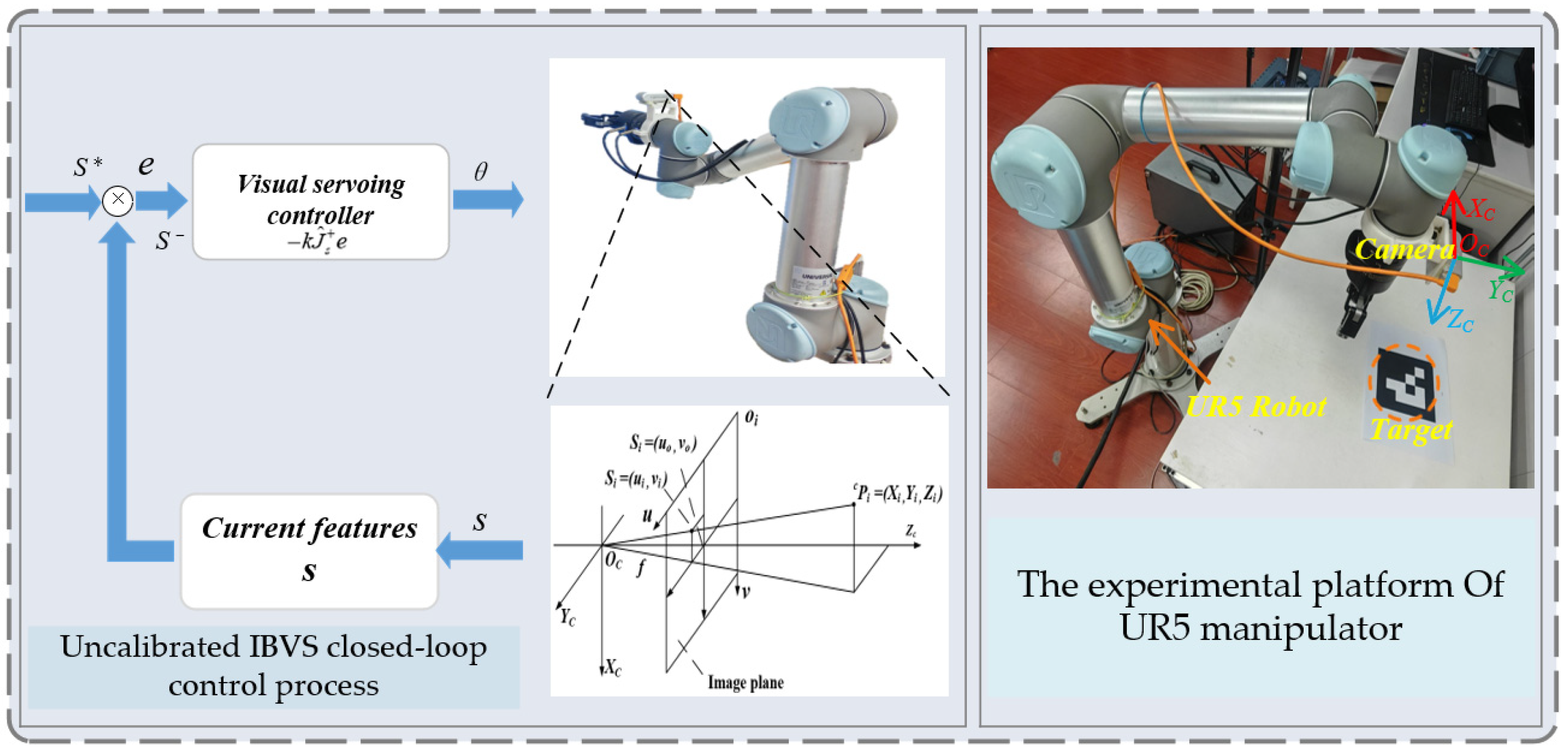
2. Theoretical Description of Uncalibrated IBVS

IBVS mainly relies on the variation of features in image space to guide robot actions. In order to realize the manipulator control directly in the image space, it is first necessary to establish the mapping relationship between the manipulator’s joint vectors to the feature (image object feature vectors) and further establish the IBVS controller.

First, define the velocity vector $V_c={[v_c^T,w_c^T]}^T={[v_x,v_y,v_z,{\omega }_x,{\omega }_y,{\omega }_z]}^T$ of the hand–eye camera in the camera coordinate system. Then, the relationship between the camera velocity $V_c$ and the speed vector ${\dot{s}}_i$ of the image feature changes $s_i$ is given as follows:

$${\dot{s}}_i=J_x^i{V}_c$$

(1)

where $J_x^i\in R^{2\times 6}$ denotes the Jacobian matrix of the image feature $s_i$.

For a visual servo with n features, the problem of image-based closed-loop visual servo control can be translated into minimizing feature errors in the image plane. Set $e(t)=s(t)-s^{*}$. $s(t)\in R^{n\times 1}$ is the current image features at time t, and $s^{\ast }\in R^{n\times 1}$ is the desired image feature. Establish the relationship between the error $e(t)$ and the camera speed $V_c\in R^{6\times 1}$ through Equation (2):

$$\left\{\begin{array}{l}e(t)=J_x{V}_c\\ V_c=-{\widehat{J}}_x^{+}e(t)\end{array}\right.$$

(2)

Further, the IBVS servo controller with proportional k control is constructed by establishing the relationship between the manipulator joint speed $\dot{\theta }$ and the image feature error $e(t)$ through Equation (3):

$$\dot{\theta }={\widehat{J}}_{\theta }^{+}{V}_{\mathrm{c}}=-k{\widehat{J}}_{\theta }^{+}{\widehat{J}}_x^{+}e(t)$$

(3)

where ${\widehat{J}}_x^{+}={\left(J_x^T{J}_x\right)}^{-1}{J}_x^T\in R^{6\times 2n}$ is the Moore–Penrose pseudoinverse of the matrix $J_x\in R^{2n\times 6}$. In the 6-DOF manipulator used in this paper, ${\widehat{J}}_{\theta }^{+}={\left(J_{\theta }\right)}^{-1}\in R^{6\times 6}$ is the inverse of the robot Jacobian matrix $J_{\theta }\in R^{6\times 6}$, and $\dot{\theta }\in R^{6\times 1}$ is the manipulator joint velocity vector.

Equation (3) can be further expressed as follows:

$$\dot{\theta }=-k{{\widehat{J}}_s}^{+}e(t)$$

(4)

In Equation (4), ${{\widehat{J}}_s}^{+}={\widehat{J}}_{\theta }^{+}{\widehat{J}}_x^{+}$, ${\widehat{J}}_s^{+}\in R^{6\times 2n}$ is called the Moore–Penrose pseudoinverse of the feature–motion mapping matrix $J_s\in R^{2n\times 6}$. For 6-DOF manipulator IBVS tasks, in order to reflect the overall relative motion relationship between the manipulator and the object, at least three features are generally required, hence the matrix (n ≥ 3).

To implement image-based uncalibrated visual servoing control, a Kalman state estimation model is required to solve the feature–motion mapping matrix $J_s$ in real time [34,35]. The Kalman state estimation model, established based on the auxiliary dynamic system, is primarily divided into two parts, an estimation of the matrix $J_s$ and a correction of the matrix $J_s$, based on the feedback of feature S changes from the observer. In uncalibrated IBVS, when using Kalman estimation to solve the matrix $J_s$, estimation errors and the limited FOV of the camera may cause the features to deviate from the camera’s FOV, leading to feature loss, especially in unknown noisy environments. To ensure the visibility of visual features in uncalibrated IBVS, specific feature constraints are required. A detailed analysis of this will be provided in the following sections.

3. Design and Training Methods for DQN Feature Constrained Control

This section will introduce the reinforcement learning approach for designing feature constraint control in the DQN. Specifically, based on the feature mapping in the offline camera FOV environment, we designed the state space, action space, and reward function to construct a feature-constrained Q-network. In order to further optimize the training process, we introduced a copy network for the Q-network and used this to train a Q-network with stable feature constraint planning capability.

First, for the IBVS task involving multidimensional features, the task needs to be formulated as a Markov decision process (MDP) model with specific tuples (S, A, P, r, λ), where P denotes the probability of transmutation, and λ denotes the discount factor for receiving a reward and is a constant. Second, according to the mechanism of DQN interaction with the environment, the (S, A, r, S′) tuple is stored in the DQN’s experience pool, and, therefore, the information of the Markov decision model elements S, A, r needs to be focused on, where S′ denotes the next state reached by the agent after executing an action in the current state S. The selection of the division of the state space S, the definition of the action space A, and the definition of the r-reward mechanism function are the key steps in using reinforcement learning as a practical task. Based on the DQN reinforcement learning, the details of each component in the tuple (S, A, r) are analyzed as follows:

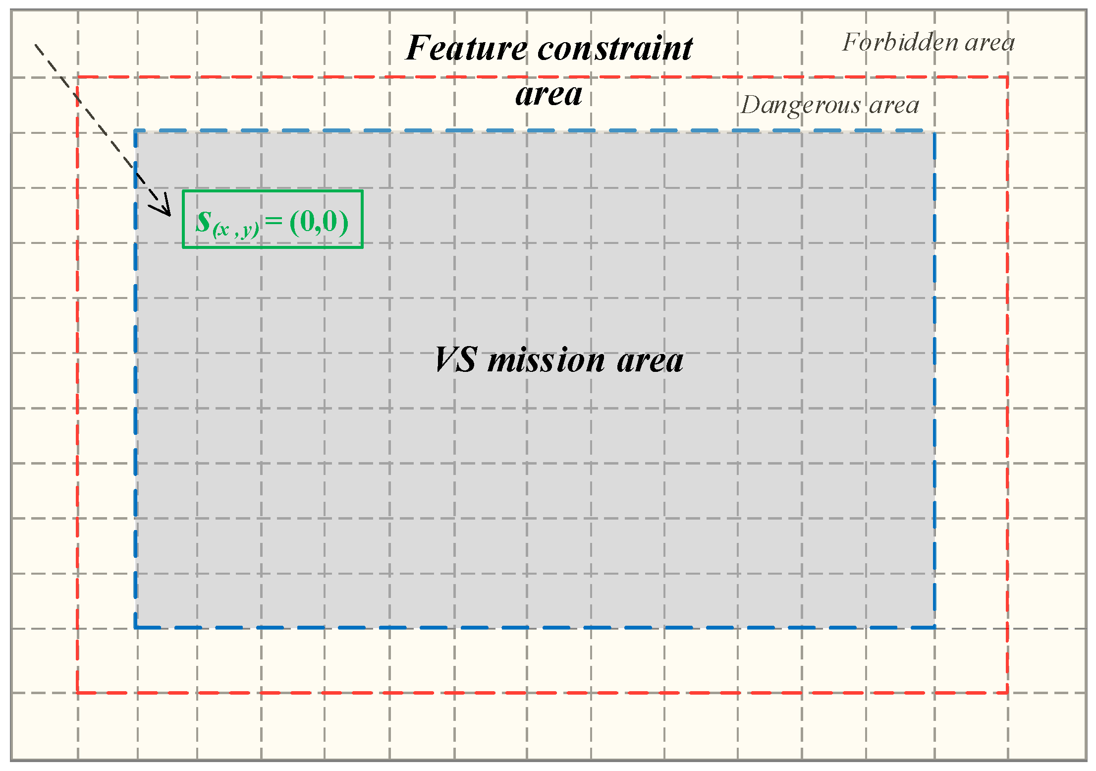
3.1. Definition and Division of State Space

To address the real-time nature of the IBVS task, we discretize the high-dimensional camera image space and build an offline camera FOV environment to map visual features to state S. This state S is used as an input to the Q-network. Further, the Q-network controller can then make correct feature constraint decisions based on the current state S. Thus, the input state of this Q-network learning is defined as shown in Figure 1. Firstly, the camera image plane is discretely divided into a space of grid, and the two main regions of grid space feature constraints and visual servoing (VS) are defined, where the feature constraint region is further categorized into dangerous area and forbidden area based on the distance from the camera FOV boundary. Then, the Q-network input environment state is given by the following equation:

$$\left\{\begin{array}{l}x=\mathrm{int}\left(u\times {\displaystyle \frac{m_u}{(u_{\max }-u_{\min })+1}}\right)\\ y=\mathrm{int}\left(v\times {\displaystyle \frac{n_v}{(v_{\max }-v_{\min })+1}}\right)\end{array}\right.$$

(5)

where (u, v) are the pixel coordinates on the image plane, with u_max and u_min representing the upper and lower limits of the horizontal axis, and v_max and v_min representing the upper and lower limits of the vertical axis. Further, the state set $S=\left\{s_{\left(\mathrm{x},y\right)}|s_{\left(x,y\right)}=\left(x,y\right)\right\}$ is obtained from Equation (5). Namely, S denotes the state space related to the point feature (Agent) in the camera FOV grid environment.

The state S is defined by the grid position S_{(x, y)} = (x, y), as depicted in Figure 1. Through Equation (5), the pixel coordinates (u, v) of the point feature in the actual camera FOV resolution image are transformed into the position S_{(x, y)} = (x, y) in the grid environment. Namely, S_{(x, y)} = (x, y) represents the state of the point feature (Agent) in the grid environment. Regarding state transitions, we define the transition probability function P(S, a) to describe how the state of the Agent changes when an action a is applied in the grid environment. Specifically, the Agent moves within the grid environment according to the selected action, and the new state is determined by the Agent’s new position S’_{(x, y)} after executing the action. For reward shaping, we assign higher reward values to states within the VS mission area, which helps guide the Agent to train more effectively, thereby achieving the goal of constraining the point feature’s coordinates in the actual camera FOV.

3.2. The Definition of Action Space

In fact, we define the Agent here as the features within the camera FOV, and the actions of these features, as they move within the FOV, are reflected in the movement of the hand–eye camera. Consequently, to constrain the features within the camera FOV, the spatial displacement of the manipulator’s hand–eye camera is directly controlled to ensure the features remain within the FOV. Let the current speed of the manipulator’s eye-in-hand camera be $V_c\in R^{6\times 1}$. Due to the discrete nature of the DQN control, the following five action velocities are defined to control the displacement of the manipulator’s eye-in-hand camera’s FOV:

(1)

Action1: $a_1=V_c^{down}$, camera FOV shifted down (features shifted upward);

(2)

Action2: $a_2=V_c^{up}$, camera FOV shifted upward (features shifted down);

(3)

Action3: $a_3=V_c^{left}$, camera FOV left shifted (features right shifted);

(4)

Action4: $a_4=V_c^{right}$, camera FOV right shifted (features left shifted);

(5)

Action5: camera FOV does not move (action5, features do not move): $a_5=V_c^s$.

For the output of above five actions, DQN controls the camera’s velocity according to whether the feature’s state S is in the visual servoing (VS) mission area or not. Specifically, in the feature constraint area, actions 1–4 are used to adjust the camera’s movement to keep the feature within the FOV. In the VS mission area, action 5 indicates that no correction to the camera’s velocity is needed, i.e., the camera’s velocity remains unchanged. Thus, the actual output action space can be obtained as $A=\left\{a_i\left|i=1,\dots ,5\right.\right\}$.

3.3. Design of the Reward Function

After defining the action space A for DQN to control moving features, the environment computes the corresponding reward r based on the feature’s state S in the offline camera FOV environment. The computation of reward r is given by the following equation:

$$r=\left\{\begin{array}{cc}-R,& if{s}_{(x,y)}\in \mathrm{outside}\mathrm{the}\mathrm{field}\mathrm{of}\mathrm{view}\hfill \\ -R/2,& if{s}_{(x,y)}\in \mathrm{the}\mathrm{forbidden}\mathrm{area}\hfill \\ 0,& if{s}_{(x,y)}\in \mathrm{the}\mathrm{dangerous}\mathrm{area}\hfill \\ R,& if{s}_{(x,y)}\in \mathrm{VS}\mathrm{mission}\mathrm{area}\hfill \end{array}\right.$$

(6)

where R is the maximum reward value, which is a positive constant. As can be seen from Figure 1 and Equation (6), the designed reward function aims to encourage the features to perform the correct actions, thereby ensuring that the features are maintained within the VS mission area (the desired region of the camera’s FOV).

After designing the state set S, action set A, and reward function r, the Q-network needs to be trained to implement the feature constraint control based on DQN. The specific training methods and results will be provided in the following chapter.

3.4. Training Method and Result

Based on the previous section, the DQN Agent (point feature) selects the linear velocity vector in the x and y directions of the camera’s coordinate system as the output action, and five discrete actions, labeled a₁ to a₅, are designed around the velocity vectors in these two directions. Additionally, the virtual camera FOV environment used for training the Q-network is also a discrete grid space, and discrete point feature displacement actions are employed. This enables the DQN model, based on a discrete action space, to efficiently learn the feature constraint strategy through the Q-learning mechanism.

The Q-network is essentially trained to learn using neural network learning to obtain the action value function

$$Q^{\pi }(s_t,a_t)=r_t+\gamma Q^{\pi }(s_{t+1},\pi (s_{t+1}))$$

(7)

This equation represents the Q-value of taking the action a_t at the time t for the Agent’s state s_t. $\pi (s_{t+1})=\underset{a_{t+1}}{{\displaystyle \max }}{Q}^{\pi }(s_{t+1},a_{\mathrm{t}+1})$ represents the optimal action a_t+1 taken at the time t + 1 for the Agent’s state s_t+1. In order to realize the feature constraint control of the DQN method, we construct a Q-network to estimate the function $Q^{\pi }(s_t,a_t)$, while a target network is used to update the weight parameter θ of the Q-network, facilitating the convergence of the Q-network gradients. The target network is a replica network of the former, and we specify the weight parameter of the target network as ${\theta }^{-}$ to distinguish it. The control of hand–eye camera movements based on Agent (feature) FOV states S is based on the $Q^{\pi }(s_t,a_t)$ function, which is actually outputted by the Q-network as $Q_{{\theta }_i}^{\pi }(s_t,a_t)$, and by the target network as $Q_{{\theta }_i^{-}}^{\pi }(s_{t+1},a_{t+1})$. During the training of the two networks, the output of the target network $Q_{{\theta }_i^{-}}^{\pi }(s_{t+1},a_{t+1})$ is used to calculate the target value $y=r_t+\delta Q_{{\theta }_i^{-}}^{\pi }(s_{t+1},\pi (s_{t+1}))$, while the output of the Q-network $Q_{{\theta }_i}^{\pi }(s_t,a_t)$ serves as the predicted value. Then, the process of updating the Q-network weight θ is as follows:

$$L({\theta }_i)={\displaystyle \frac{1}{N}}{\displaystyle \sum _{i=1}^N{\left(y-Q_{{\theta }_i}^{\pi }(s_t,a_t)\right)}^2}$$

(8)

$${\theta }_i\leftarrow {\theta }_i+\alpha \nabla L(\theta )$$

(9)

$$\nabla L({\theta }_i)={\displaystyle \frac{1}{N}}{\displaystyle \sum _{i=1}^N\nabla {\left(y-Q_{{\theta }_i}^{\pi }(s_t,a_t)\right)}^2}$$

(10)

Another important technique to address the issue of non-independent and non-identically distributed training samples is experience replay. By utilizing a replay buffer (the experience pool) that stores past experiences (namely S, A, r, S′), this method allows for the mixing of past and current experiences. This reduces the correlation between data points and enables the reuse of samples, ultimately enhancing the learning efficiency. In the above Equations (8) and (10), N denotes the number of sample batches obtained from the experience pool, and α is the learning rate. For the target network, parameter ${\theta }^{-}$ is not updated in real time; the target network is assigned the parameter after the Q-network parameter is updated for a period of time; then, it can be expressed by Equation (11):

$${\theta }_i^{-}\leftarrow {\theta }_i$$

(11)

The Q-network interacts with the environment multiple times through the above process and learns to obtain the optimal action-value function, $Q_{{\theta }_i}^{\pi }(s_t,a_t)$. With function $Q_{{\theta }_i}^{\pi }(s_t,a_t)$, the visual feature as Agent can use the ε-greedy policy to select the optimal action strategy $\pi (s_t)=\arg \underset{a_t}{\max }{Q}_{{\theta }_i}^{\pi }(s_t,a_t)$ and control the camera movement to keep visual features within the camera’s safe FOV with strategic action $\pi (s_t)$. The training method for the Q-network based on the offline camera FOV environment is as follows (Algorithm 1):

Algorithm 1: Q-Network Training

Define the camera FOV environment, state space S, action space A, and r reward functions; Set up and initialize Q-network (primary network) and target network parameter ${\theta }_i,{\theta }_i^{-}$; Initialize learning rate α, discount factor γ, exploration rate ϵ; for episode = 1, …, n do  Randomly initialize the feature’s state (positions) in the camera FOV  and observe the initial state $s_{\left(x,y\right)}$; for t = 1, …, m do  Acquire state $s_t=s_{(x,y)}$ and select actions from A based on ε-greedy policy;  Get reward $r_t$ and reach new state $s_{t+1}$;  Store sample $\left(s_t,a_t,r_t,s_{t+1}\right)$ into the replay buffer D;  if $s_{t+1}$ is located in VS area then   break;  if D is full then   Extract N samples from D according to Equations (8)–(11)   Update network Q-network and target network parameters ${\theta }_i,{\theta }_i^{-}$;  end if  end for end for Optimal action value function Q based on FOV feature constraints (trained Q-network)

In order to realize the Q-network to control the displacement of features according to the feature state in the python-based PyCharm environment, construct a Q-network, as well as target networks with the same structure. The structure of these two networks is a two-layer fully connected neural network with a hidden layer containing 50 neurons, each followed by a ReLU activation function. Then, set the network learning rate to α = 0.01 and the reward discount factor to γ = 0.99. To ensure feature path exploration and optimal action selection, set the greedy policy to ϵ = 0.2; set the replay buffer D to size 150 and the training extracted data batch N to size 32 for training learning of the Q-network. Meanwhile, to simulate the actual camera FOV environment, we followed the scheme outlined in Section 3. The 640 × 480 camera plane was further segmented, and a virtual camera FOV environment of size 16 × 16 was constructed within the PyCharm environment. In this environment, based on the design principles of the action set A and reward function r in Section 3, we trained the Q-network to guide the movement of the feature. Specifically, the purpose of our offline training is to guide the Agent (point features) in the FOV environment to follow the principle of reward function into VS mission area.

The specific offline training process is shown in Figure 2. During the training process in the grid environment based on the virtual camera FOV, the position of the Agent is defined as the state s, and its movement direction is defined as the action a. Partitions with different reward values, r, are set up according to the point feature FOV rules. During training, the Agent interacts with the environment in the simulation to generate experience data (s, a, r, s′), which are stored in the experience memory pool. Both the target network and the Q-network sample data from this pool to compute the target Q-value and the current Q-value. These are used to construct the loss function, which incorporates the immediate reward r. Ultimately, the Q-network optimizes the Q-value function through gradient descent to learn the policy that constrains the Agent’s behavior. In this training experiment, the Q-network was trained for 500 iterations, resulting in the averaged controller rewards shown in Figure 3. From the figure, it can be observed that the reward value continues to increase after several training sessions, and the average cumulative reward curve tends to asymptotically converge, which indicates that the Q-network can be trained to constrain the features based on the offline camera FOV environment to ensure the visibility of the features in the camera FOV. Further, after training a good Q-network, we can migrate it to the real manipulator IBVS environment for feature constrained control.

To observe the Q-value of the feature’s action when it is in a particular FOV state S, Figure 4 records the history of Q-value changes after 500 iterations of training the Q-network. In Figure 4a, it can be observed that for the visual features in the camera FOV state (3,1), the action (Down) has a higher Q-value compared to the other four actions. This means that the action (Down) has a higher probability to be selected by the Agent (features) when the feature is in the camera FOV’s dangerous and forbidden areas. That is, the camera is controlled to perform an action that moves the features down into the VS mission area, thereby constraining the features within the camera’s safe field-of-view. Similar conclusions can be drawn from Figure 4b. The Q-network learning is actually a behaviour-based decision-making unit that possesses a self-learning mechanism for real-time interaction with the environment, in contrast to the potential method discussed in [21,22,23,26]. For the multidimensional feature-constrained control task, the use of neural network learning simplifies task complexity compared to the traditional Q-learning method in [29], which maintains a Q table.

In order to realize the uncalibrated visual servoing task with feature constraint, we designed and trained a feature-mapped Q-network for the offline camera FOV environment. If the feature-constrained Q-network is applied to practical uncalibrated visual servoing tasks, the overall visual servoing system architecture and design should not depend on system’s specific configuration. Around this, in the following sections we will build the uncalibrated visual servoing framework with DQN feature constraints.

4. DQN-Based Visual Servoing with FOV Feature Constraints

Based on the establishment and training of the Q-network in the previous section, we constructed the DQN-based uncalibrated IBVS framework, in which we employ the Kalman filter for mapping matrix estimation, as we did in our previous works [36]. The proposed overall framework is shown in Figure 5, and the overall framework contains a total DQN feature constraint module, feature–motion mapping matrix estimation module, and image processing module. For the image processing module, the main function is to receive the camera image information to extract the object feature S. The estimator’s function in the mapping matrix estimation module is to calculate the matrix $J_s$ based on the real-time feature $S$.

For the DQN module, the operation mechanism of its main body is consistent with Figure 2. However, to better integrate with the actual uncalibrated visual servoing task, we apply feature screening to the real-time multidimensional feature information S from the camera. For the uncalibrated visual servoing task of the 6-DOF manipulator, the number of features used are generally n ≥ 3. When there are multiple features in the camera’s FOV, if any feature is close to the boundary line between the VS mission area and the constrained area of features, as depicted in Figure 1, the method in Figure 6 always ensures finding a feature closest to that boundary line, and this feature is used as the object of the DQN module constraint, thus realizing FOV constraint control for each feature in the visual servoing task. In addition, for the action output of the DQN feature constraint module, the joint velocities $\dot{\theta }=\widehat{J}{\left(\theta \right)}^{+}{V}_c$ can be obtained from the output variable $V_c$ through the pseudoinverse $\widehat{J}{\left(\theta \right)}^{+}$ of the manipulator’s Jacobian matrix. Joint variables ${\theta }_{DQN},\dot{\theta }$ are obtained with numerical integration and differentiation. When the output ${\theta }_{KFIBVS}$ controls the hand–eye camera, causing the feature to enter the camera’s FOV danger area (feature constraint area) and potentially escape the FOV, the DQN constraint module adaptively outputs a constraint complementary variable ${\theta }_{DQN}$, which constrains the feature within the FOV’s safe area (VS mission area).

In the framework we designed, we consider three sources of delay in the DQN component: (1) the processing time for converting visual features from the camera’s virtual FOV environment into state variables; (2) the computation time required for the Q-network to infer appropriate constraint actions; and (3) the process of converting the DQN output actions into robot joint variables. We set the sampling frequency of the uncalibrated IBVS controller to 2.5 Hz (i.e., the controller calculates new control inputs every 0.4 s and sends them to the robot for execution) to ensure smooth control of the robot. Therefore, the time from receiving the state to generating an action in the DQN component must also be synchronized with the IBVS controller. If the DQN computation delay is too long and cannot be synchronized with the sampling frequency of the IBVS controller, the constraint actions generated by DQN may lag behind the IBVS control output, leading to inaccurate control commands for the robot. Especially in real-time applications, the accumulation of delays may affect the system’s stability and convergence speed.

5. Experimental Results

In this subsection, experiments are designed to verify the effectiveness of the proposed control method in a real scenario. Figure 7 shows the task environment in which the manipulator of the UR5 moves close to the target. Specifically, the manipulator acquires the visual features S of the target in real-time through the end-mounted Realsensed 435i camera and feeds them back to the located PC, which further sends the IBVS control commands to the UR5 manipulator controller. The camera captures video at a resolution of 640 × 480 pixels and feeds the acquired image data into the Visp image processing library program in Visual Studio 2017. The program extracts the feature center coordinates at a sampling interval of 0.01 s and sends them to the IBVS controller, implemented in MATLAB R2016b on the PC side, for processing. In the practical experiments, we established the DQN-based uncalibrated visual servoing framework. Within the established framework, the Q-networks were trained as expected; as described in Section 3.4, the task is to control the manipulator from an arbitrary initial pose to the desired pose by using the proposed uncalibrated IBVS system with closed-loop feedback of image features. The manipulator takes the features of the QR code target’s four corner points on the platform as input, which are labeled A, B, C, and D in the experiment. The current feature is obtained as $S=\left[s_1,s_2,s_3,s_4\right]\in R^{8\times 1},s_i=\left(u_i,v_i\right),i=1,2,3,4.$, and the manipulator control variable is $\theta \in R^{6\times 1}$. The Q-network parameters in the DQN feature-constrained control module are the same as the training parameters in 3–4. Note that in the DQN feature constraint section, the actual input state is $s_i$.

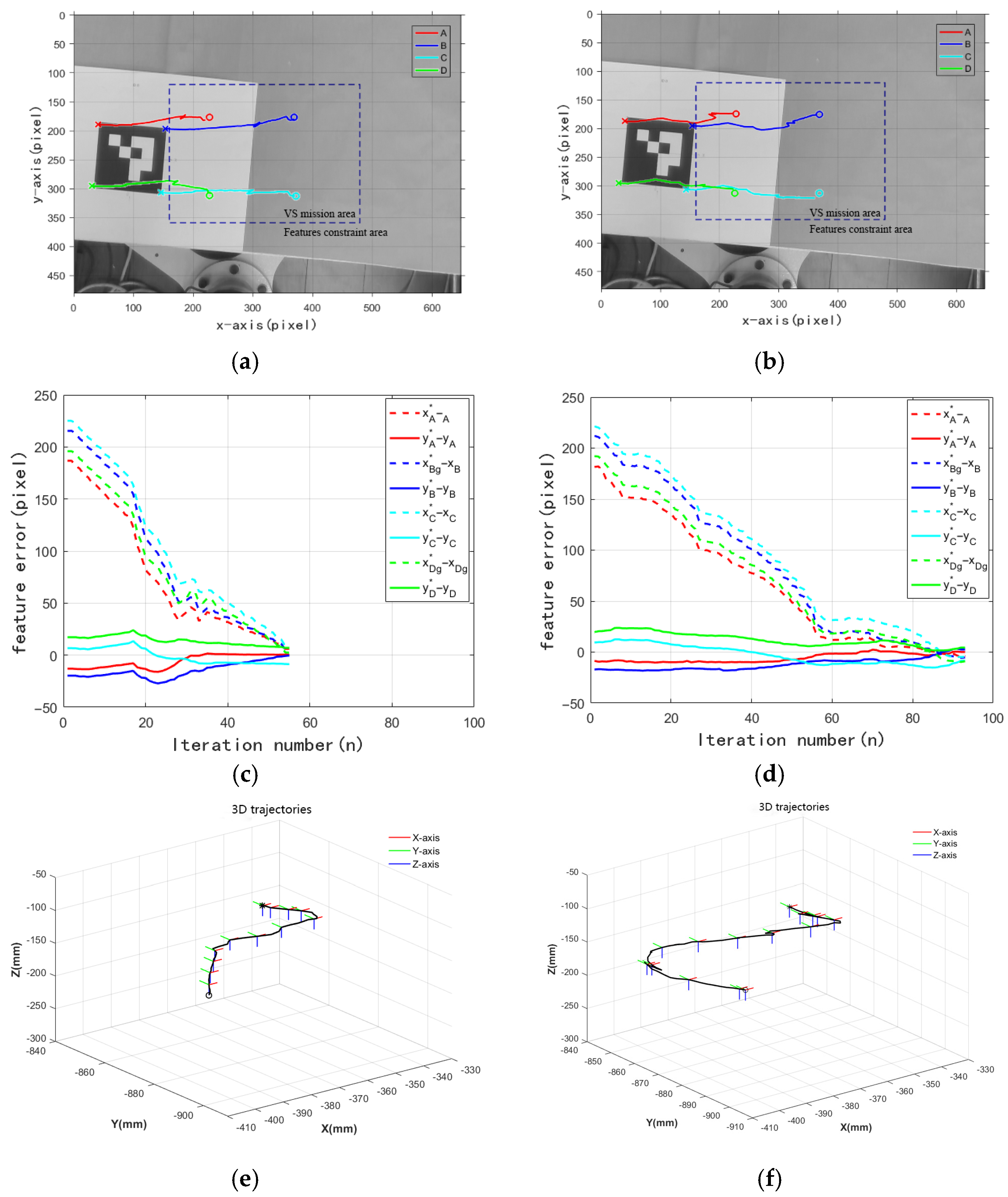
5.1. Features Constraint Validation

In order to validate the effectiveness of the feature constraints in our proposed DQN feature constraint scheme, two sets of experiments are conducted and described in detail in the following sections.

Test 1: In this section of the experiment, the initial image features were set outside the VS mission area, in which the VS mission area is defined as (80–559) × (120–359). To verify the scalability of the proposed feature constraint control, experiments were conducted using two different initial feature states (positions) within the feature constraint area. The experimental results are presented in Figure 8a,b, demonstrating that the DQN feature constraint control scheme effectively constrains the features, whose initial states are within the feature constraint region, to the VS mission area. Additionally, the constraint curves exhibit a relatively straight trajectory. From Figure 8c,d, it can be observed that in the DQN constraint control phase, the error convergence curves of the four features in the longitudinal direction are relatively smooth, with error values decreasing between 0 and 16 iterations. This result further indicates that the proposed DQN constraint control effectively handles the feature constraint task without compromising the convergence of visual servoing adaptivity. The 3D trajectory of the manipulator end-effector equipped with a hand–eye camera in Cartesian space is illustrated in Figure 8e,f. It can be observed that after the feature constraint action at the initial state positions, the overall convergence trajectory remains relatively smooth.

Test 2: Verifying the feature constraint control capability of the DQN module during the servoing process. In this part of the experiment, the VS mission area was set to (0–559) × (0–359) and (0–559) × (120–480). Figure 9 illustrates the experimental results for two different sets of initial and desired feature states.

As shown in Figure 9a,b, the constraint control of the DQN module is activated to correct the IBVS trajectory if the features at different initial states move outside the safe region (VS mission area) during servo motion. In Figure 9c,d, it can be observed that within the intervals from 150 to 155 in (c) and from 10 to 20 in (d), the DQN module facilitates the convergence of the error between the desired and target features while maintaining feature visibility constraints. As can be seen in Figure 9e,f, the spatial convergence trajectory is more complicated when features appear to exceed the VS mission area during visual servoing. This can be considered as a large error in the feature–motion mapping matrix estimated by the Kalman mapping matrix estimator due to unknown environmental noise disturbances, which further leads to more complex control trajectories output by the visual servo controller. In this case, when features move beyond the VS mission area, the DQN module’s feature constraint control is activated to pull them back into the VS mission area, ensuring the visual servoing task achieves convergence.

5.2. Comparison Experiment

To verify the feature constraint capability of the proposed DQN feature constraint visual servo under different noise environments, we conducted feature constraint experiments in three different noise environments and compared the results with those of the Kalman visual servo without feature constraints. We set the initial feature’s state to $S=\left[229.7,172.9,371.9,174.3,372.0,312.2,225.6,309.3\right]$, and the desired feature’s state to $S^{*}=\left[46.4,179.0,160.4,187.1,152.0,299.7,34.5,286.5\right]$. Meanwhile, in order to better compare the two methods’ convergence effects, we set the VS mission area as (160–479) × (120–359).

Test 1: We introduced noise of varying intensities into the system and validated the servoing performance of both the Kalman-DQN visual servo and the Kalman visual servo under different noise conditions. In experiment text1, we set the system noise covariance to $Q=0.9I_{48\times 48}$ and the observation noise covariance to $R=0.01I_{8\times 8}$, respectively. As observed in Figure 10a,b, when the initial feature’s state is within the feature constraint region, the proposed DQN feature constraint control is activated. The DQN module’s control effectively compensates for the convergence of the visual servo, resulting in a relatively smooth trajectory within the feature constraint region compared to (b). In contrast, the Kalman visual servo in (b), lacking the compensation from the DQN module’s feature constraint, exhibits weaker convergence performance due to the influence of noise on the Kalman estimator, leading to a relatively more curved trajectory. Comparison of (c,d) and (e,f) leads to the conclusion that our proposed visual servoing scheme has faster convergence and better spatial trajectory curves.

Test 2: The spatial trajectories of the end-effector with camera and the image plane convergence trajectories when $Q=4I_{48\times 48},R=0.04I_{8\times 8}$ are given in Figure 11. The results show that the overall image convergence trajectory and spatial convergence trajectory of our proposed method still outperform the Kalman visual servo without feature constraints due to the feature constraint compensation effect in the presence of increased noise, which further demonstrates the stabilizing property with robustness. In terms of convergence time, Figure 11c,d show that our method converges faster.

Test 3: When increasing the noise setting to $Q=9I_{48\times 48},R=0.09I_{8\times 8}$, as shown in Figure 12, due to the increased Jacobian matrix error in the Kalman estimation, there is a larger camera back-off in the workspace, which further increases the clutter in both the spatial convergence trajectory and the image plane convergence trajectory. However, in the face of the same noise, for our proposed DQN feature constraint visual servoing method, the image convergence trajectory, the spatial trajectory, and the convergence speed are superior to the Kalman visual servoing without feature constraint.

Furthermore, experiments in different noise environments demonstrate that the localization results of the Kalman visual servoing without feature constraint change significantly even with slight variations in the noise covariance of Q and R. When using the DQN feature constraint as an auxiliary to the Kalman visual servoing, our proposed DQN feature constraint method not only ensures the visibility of visual features, but also, in the presence of large dynamic noise, guarantees the robust stability of the convergence task.

5.3. Ablation Study and Real Application

Previous studies [37] have shown that in complex motions involving large rotations and translations, robotic arm visual servoing tasks are prone to target features exceeding the camera’s field-of-view (FOV). To validate the effectiveness of our proposed DQN-based feature constraint module in uncalibrated IBVS tasks, we designed a series of ablation studies in challenging scenarios to compare its performance with that of uncalibrated IBVS without the DQN constraint module.

In this ablation study, the feature constraint region representing the camera’s safe FOV is set to (80–559) × (120–359). The initial and desired features we defined are as follows:

$$S=[111.29,185.20,212.88,146.42,255.64,247.87,145.20,289.65]$$

$$S^{*}=[372.82,163.67,520.18,163.07,524.10,303.29,374.52,302.60]$$

As shown in Figure 13a,c,e, under the unconstrained visual servoing control, some features exceed the camera’s FOV due to the extended convergence motion path, leading to non-convergent errors and oscillations in the spatial convergence trajectory. In contrast, Figure 13b,d,f demonstrate that our proposed DQN module successfully constrains all image features within the predefined safe FOV of the camera and achieves fast and stable convergence within the specified feature error tolerance, while also maintaining a smoother spatial convergence trajectory. This indicates that in uncalibrated IBVS tasks involving complex motion paths, image features may approach the FOV boundary or even exceed it, potentially affecting system convergence due to singularities in the feature-to-motion mapping matrix. However, our DQN-based feature constraint module in uncalibrated IBVS effectively addresses this challenge, ensuring the system’s convergence.

In order to verify the feasibility of our proposed method in practical applications, we applied the method to the task of assisted localization of a robot grasping an object, in which the experimental localization objects are randomly placed, and the Yolov8-pose object pose detection model is used to detect the actual objects as targets. The bottle cap object with the highest confidence in the first frame is selected as the target for localization and grasping during real-time detection. The object localization point feature is inferred in real-time and feedback to the DQN-based IBVS controller. The object localization and grasping when the manipulator is at the initial position and the desired position are shown in Figure 14a,b.

From the results of feature trajectory plots in Figure 14c, it is evident that with our proposed visual servoing method, the DQN feature constraint module can promptly make compensating corrections to the output of the IBVS controller. This enables the control of the manipulator to effectively draw the point features back into the visual servoing (VS) task area. Figure 14d,e illustrate that the feature convergence time of the DQN-based visual servoing is notably shorter. Additionally, the spatial trajectory of our method exhibits greater smoothness. In the robot grasping phase of visual servoing, the proposed method manages to identify a relatively ideal grabbing position. Consequently, these results demonstrate the effectiveness of the proposed method in practical robotic applications.

6. Discussion

The proposed uncalibrated IBVS system is based on the DQN feature constraint method, enabling it to fulfill the robot’s high-precision positioning tasks. In these application scenarios, the system can effectively satisfy the linearization assumption of the feature–motion velocity relationship. Therefore, the long-term stability of the system is mainly demonstrated under these large-scale operational conditions. In our tests, we evaluated the stability of the system over a certain period. The experimental results show that the system can stably converge within the specified accuracy error range, and no significant feature drift or degradation in convergence performance was observed during the convergence process.

Although DQN is primarily used for discrete control, our method adapts it by defining the action space of DQN as the linear velocity vector in the x and y directions of the camera coordinate system. These velocity vectors are then converted into corresponding joint velocity commands, which are compensated and added to the joint variables’ output by the uncalibrated IBVS controller, making it applicable to continuous motion control in a visual servoing system. In Section 5.1, we first analyze the experimental results when the initial feature state is within the camera’s FOV constraint region. The tests indicate that, along the converging path of continuous motion, the proposed method demonstrates good image feature convergence trajectories and reasonable spatial motion trajectories. Furthermore, during the servo motion, we tested the feature constraint capability of DQN. The experimental results show that when the features tend to drift out of the camera’s FOV, DQN plays a crucial role in feature constraint, enabling the uncalibrated IBVS to complete the convergence task within the specified error range.

In our experiments, we focus on the applicability of the uncalibrated IBVS under varying lighting conditions and environments with changing object texture features, though the experimental scenarios do not include obstacles. We believe that the developed method remains stable on a desktop with a textured background and in low-light environments, primarily because changes in illumination and background texture do not significantly impact the extraction of point features. It should be noted that our research focuses on image feature constraints visible within the camera’s FOV and the subsequent error-converging localization process. In the presence of obstacles, two scenarios may arise. First, during the convergence motion of the proposed system, obstacles may block the object, causing a shift or loss of image features, which can lead to task interruption. Second, if the manipulator comes into contact with an obstacle during motion, it could cause the convergence time to be indefinitely extended, prevent convergence, or stop the manipulator from advancing, potentially resulting in a task failure. To address these challenges, we plan to further investigate feature prediction and obstacle-avoidance planning to improve these aspects in our future research.

Likewise, distortion in image signals and sudden changes in lighting conditions can not only lead to erroneous actions in the DQN feature constraint control but also affect the overall performance of the uncalibrated IBVS. Specifically, a sudden increase in observation noise can result in a larger estimation error of the feature–motion mapping matrix by the Kalman filter, thereby increasing the uncertainty in IBVS motion and potentially causing task convergence failure or interruption. This occurs because the visual feedback loop obtains incorrect feature information, which in turn affects the stability of the entire control system. Therefore, it is important to develop more robust feature extraction methods for visual servoing.

Regarding changes in the input image resolution, we believe the DQN-based constraint control method remains applicable. During the training of the Q-network, the training environment can be adjusted to accommodate the new image resolution, and this adjustment does not alter the feature constraint rules set during the DQN training process. Therefore, the method remains effective. As for the increase in the number of features, our approach always selects and constrains the single point feature closest to the image boundary. Hence, regardless of the number of point features extracted from the image, the DQN control strategy continues to function effectively, ensuring that the key feature points are always maintained within the camera’s FOV.

The proposed uncalibrated IBVS is grounded in DQN feature constraint. Its convergence space generally encompasses the motion range of the robot. Our prior research work [36] has already validated its reliability over extended periods of operation in large-scale robotic tasks. Building upon this foundation, the uncalibrated IBVS system established herein satisfies feature constraints and converges stably over extended periods within a specific workspace range.

Nevertheless, we are well aware that in a more extensive and protracted convergence path, the uncalibrated IBVS may still encounter numerous challenges due to accumulated uncertainties and nonlinear effects. Consequently, future research is imperative to develop uncalibrated IBVS systems that exhibit enhanced long-term convergence stability across larger workspaces.

7. Conclusions

Aiming at the feature constraint problem in uncalibrated IBVS visual servoing in unknown noise environments, this paper proposes an new uncalibrated IBVS framework based on DQN feature constraint. the proposed DQN constraint scheme is able to accurately estimate the feature constraint decisions, thereby enforcing the FOV constraint on the Agent (features) and ensuring the stability of convergence in the visual servoing task. Additionally, the design and training of the Q-network account for the random motions of the manipulator caused by errors in the Kalman-estimated mapping matrix, which further enhances the stability of the uncalibrated IBVS system. The trained Q-network, developed in an offline environment, is integrated into a real Kalman uncalibrated manipulator IBVS system. The effectiveness of the proposed method was validated through feature constraint experiments and comparative testing. Further experiments demonstrated that the method effectively reduces the impact of noise on performance, thereby significantly enhancing the robustness of the uncalibrated IBVS system. In future research, we will further extend the method by exploring how to incorporate more significant environmental disturbances into the reinforcement learning framework and enhance its robustness and adaptability by transforming disturbance issues into learning costs. Meanwhile, the theoretical analysis of the stability of learning algorithms remains an open issue. Future research will also focus on developing a theoretical framework for neural networks and reinforcement learning to ensure the system’s convergence and stability.

References

1. Tsuchida, S.; Lu, H.; Kamiya, T.; Serikawa, S. Characteristics Based Visual Servo for 6DOF Robot Arm Control. Cogn. Cogn. Robot. 2021, 1, 76–82. [Google Scholar] [CrossRef]
2. Reyes, R.; Murrieta-Cid, R. An approach integrating planning and image-based visual servo control for road following and moving obstacles avoidance. Int. J. Control 2020, 93, 2442–2456. [Google Scholar] [CrossRef]
3. Liu, H.; Zhu, W.; Dong, H.; Ke, Y. Hybrid visual servoing for rivet-in-hole insertion based on super-twisting sliding mode control. Int. J. Control Autom. Syst. 2020, 18, 2145–2156. [Google Scholar] [CrossRef]
4. Madhusanka, B.G.D.A.; Jayasekara, A.G.B.P. Design and development of adaptive vision attentive robot eye for service robot in domestic environment. In Proceedings of the IEEE International Conference on Information and Automation for Sustainability, Celle, Sri Lanka, 16–19 December 2016; pp. 1–6. [Google Scholar]
5. Cai, K.; Chi, W.; Meng, M. A Vision-Based Road Surface Slope Estimation Algorithm for Mobile Service Robots in Indoor Environments. In Proceedings of the 2018 IEEE International Conference on Informatics, Electronics and Vision (ICIEV), Dhaka, Bangladesh, 17–19 May 2018; pp. 1–6. [Google Scholar]
6. Allibert, G.; Hua, M.; Krupínski, S.; Hamel, T. Pipeline following by visual servoing for autonomous underwater vehicles. Control Eng. Pract. 2019, 82, 151–160. [Google Scholar] [CrossRef]
7. Shu, T.; Gharaaty, S.; Xie, W.; Joubair, A.; Bonev, I. Dynamic path tracking of industrial robots with high accuracy using photogrammetry sensor. IEEE/ASME Trans. Mechatron. 2018, 23, 1159–1170. [Google Scholar] [CrossRef]
8. Janabi-Sharifi, F.; Deng, L.; Wilson, W.J. Comparison of Basic Visual Servoing Methods. IEEE/ASME Trans. Mechatron. 2010, 16, 967–983. [Google Scholar] [CrossRef]
9. Wu, J.; Jin, Z.; Liu, A.; Yu, L. Non-linear model predictive control for visual servoing systems incorporating iterative linear quadratic Gaussian. IET Control Theory Appl. 2020, 14, 1989–1994. [Google Scholar] [CrossRef]
10. Malis, E.; Chaumette, F.; Boudet, S. 2 1/2 D visual servoing. IEEE Trans. Robot. Autom. 1999, 15, 238–250. [Google Scholar] [CrossRef]
11. Tang, Z.; Cunha, R.; Cabecinhas, D.; Hamel, T.; Silvestre, C. Quadrotor going through a window and landing: An image-based visual servo control approach. Control Eng. Pract. 2021, 112, 104827. [Google Scholar] [CrossRef]
12. Chaumette, F.; Hutchinson, S. Visual servo control. I. Basic approaches. IEEE Robot. Autom. Mag. 2006, 13, 82–90. [Google Scholar] [CrossRef]
13. Siradjuddin, I.; Behera, L.; McGinnity, T.; Coleman, S. Image-based visual servoing of a 7-DOF robot manipulator using an adaptive distributed fuzzy PD controller. IEEE/ASME Trans. Mechatron. 2013, 19, 512–523. [Google Scholar] [CrossRef]
14. Ahmadi, B.; Xie, W.-F.; Zakeri, E. Robust cascade vision/force control of industrial robots utilizing continuous integral sliding-mode control method. IEEE/ASME Trans. Mechatron. 2022, 27, 524–536. [Google Scholar] [CrossRef]
15. Gao, J.; Proctor, A.A.; Shi, Y.; Bradley, C. Hierarchical model predictive image-based visual servoing of underwater vehicles with adaptive neural network dynamic control. IEEE Trans. Cybern. 2016, 46, 2323–2334. [Google Scholar] [CrossRef]
16. Li, Z.; Yang, C.; Su, C.; Deng, J.; Zhang, W. Vision-based model predictive control for steering of a nonholonomic mobile robot. IEEE Trans. Control Syst. Technol. 2016, 24, 553–564. [Google Scholar] [CrossRef]
17. Maniatopoulos, S.; Panagou, D.; Kyriakopoulos, K.J. Model Predictive Control for the Navigation of a Nonholonomic Vehicle with Field-of-View Constraints. In Proceedings of the 2013 American Control Conference, Washington, DC, USA, 17–19 June 2013; pp. 3967–3972. [Google Scholar]
18. Huang, X.; Houshangi, N. A Vision-Based Autonomous Lane Following System for a Mobile Robot. In Proceedings of the 2009 IEEE International Conference on Systems, Man, and Cybernetics, San Antonio, TX, USA, 11–14 October 2009; pp. 2344–2349. [Google Scholar]
19. Wang, R.; Zhang, X.; Fang, Y.; Li, B. Virtual-goal-guided RRT for visual servoing of mobile robots with FOV constraint. IEEE Trans. Syst. Man Cybern. Syst. 2021, 52, 2073–2083. [Google Scholar] [CrossRef]
20. Heshmati-Alamdari, S.; Karras, G.C.; Eqtami, A.; Kyriakopoulos, K.J. A Robust Self-Triggered Image-Based Visual Servoing Model Predictive Control Scheme for Small Autonomous Robots. In Proceedings of the IEEE/RSJ International Conference on Intelligent Robots and Systems (IROS), Hamburg, Germany, 28 September 28–2 October 2015; pp. 5492–5497. [Google Scholar]
21. Chesi, G. Visual Servoing Path Planning via Homogeneous Forms and LMI Optimizations. IEEE Trans. Robot. 2009, 25, 281–291. [Google Scholar] [CrossRef]
22. Kazemi, M.; Gupta, K.; Mehrandezh, M. Global Path Planning for Robust Visual Servoing in Complex Environments. In Proceedings of the 2009 IEEE International Conference on Robotics and Automation, Kobe, Japan, 12–17 May 2009; pp. 326–332. [Google Scholar]
23. Corke, P.I.; Hutchinson, S. A New Partitioned Approach to Image-Based Visual Servo Control. IEEE Trans. Robot. Autom. 2001, 17, 507–515. [Google Scholar] [CrossRef]
24. Chen, J.; Dawson, D.M.; Dixon, W.E.; Chitrakaran, V.K. Navigation Function-Based Visual Servo Control. Automatica 2007, 43, 1165–1177. [Google Scholar] [CrossRef]
25. Cowan, N.J.; Weingarten, J.D.; Koditschek, D.E. Visual Servoing via Navigation Functions. IEEE Trans. Robot. Autom. 2002, 18, 521–533. [Google Scholar] [CrossRef]
26. Zheng, D.; Wang, H.; Wang, J.; Zhang, X.; Chen, W. Toward visibility guaranteed visual servoing control of quadrotor UAVs. IEEE/ASME Trans. Mechatron. 2019, 24, 1087–1095. [Google Scholar] [CrossRef]
27. Hajiloo, A.; Keshmiri, M.; Xie, W.F.; Wang, T.T. Robust Online Model Predictive Control for a Constrained Image-Based Visual. Servoing. IEEE Trans. Ind. Electron. 2016, 63, 2242–2250. [Google Scholar]
28. Sutton, R.S.; Barto, A.G. Reinforcement Learning: An Introduction; The MIT Press: Cambridge, MA, USA, 2018. [Google Scholar]
29. Wang, Y.; Lang, H.; De Silva, C.W. A Hybrid Visual Servo Controller for Robust Grasping by Wheeled Mobile Robots. IEEE/ASME Trans. Mechatron. 2010, 15, 757–769. [Google Scholar] [CrossRef]
30. Wu, J.; Jin, Z.; Liu, A.; Yu, L.; Yang, F. A Hybrid Deep-Q-Network and Model Predictive Control for Point Stabilization of Visual Servoing Systems. Control. Eng. Pract. 2022, 128, 105314. [Google Scholar] [CrossRef]
31. Shi, H.; Li, X.; Hwang, K.S.; Pan, W.; Xu, G. Decoupled Visual Servoing with Fuzzy Q-Learning. IEEE Trans. Ind. Inform. 2018, 14, 241–252. [Google Scholar] [CrossRef]
32. Shi, H.; Shi, L.; Sun, G.; Hwang, K.S. Adaptive Image-Based Visual Servoing for Hovering Control of Quad-Rotor. IEEE Trans. Cogn. Dev. Syst. 2020, 12, 417–426. [Google Scholar] [CrossRef]
33. Jin, Z.; Wu, J.; Liu, A.; Zhang, W.A.; Yu, L. Policy-based deep reinforcement learning for visual servoing control of mobile robots with visibility constraints. IEEE Trans. Ind. Electron. 2021, 69, 1898–1908. [Google Scholar] [CrossRef]
34. Xiaolin, R.; Hongwen, L. Uncalibrated image-based visual servoing control with maximum correntropy Kalman filter. IFAC-PapersOnLine 2020, 53, 560–565. [Google Scholar] [CrossRef]
35. Jiao, J.; Li, Z.; Xia, G.; Xin, J.; Wang, G.; Chen, Y. An uncalibrated visual servo control method of manipulator for multiple peg-in-hole assembly based on projective homography. J. Frankl. Inst. 2025, 362, 1234–1249. [Google Scholar] [CrossRef]
36. Zhong, X.; Zhong, X.; Peng, X. Robots visual servo control with features constraint employing Kalman-neural-network filtering scheme. Neurocomputing 2015, 151, 268–277. [Google Scholar] [CrossRef]
37. Chaumette, F. Potential problems of stability and convergence in image-based and position-based visual servoing. In The Confluence of Vision and Control; Springer: London, UK, 2007; pp. 66–78. [Google Scholar]
Figure 1. Discrete camera field-of-view environment.
Applsci 15 04447 g001
Figure 2. Q-network training flow based on offline camera FOV environment.
Applsci 15 04447 g002
Figure 3. Average cumulative reward over episodes.
Applsci 15 04447 g003
Figure 4. Q-value recordings of features at different FOV states S, in an offline camera FOV environment. (a) Q-value record of features at state (3, 1), (b) Q-value record of features at state (1, 6).
Applsci 15 04447 g004
Figure 5. The proposed DQN-based uncalibrated IBVS framework.
Applsci 15 04447 g005
Figure 6. Multidimensional feature screening.
Applsci 15 04447 g006
Figure 7. UR5 manipulator experimental platform.
Applsci 15 04447 g007
Figure 8. When the VS mission area is (80–559) × (120–359), the constraint control results for features at different initial states in the feature constraint area are shown. (a,b) present the convergence trajectories, (c,d) illustrate the convergence errors, and (e,f) depict the end-effector trajectories.
Applsci 15 04447 g008
Figure 9. Constrained features during the visual servoing convergence process in the VS mission area (0–559) × (0–359) and (0–479) × (120–480). (a,b) show the convergence trajectories, (c,d) illustrate the convergence errors, and (e,f) depict the end-effector trajectories, all when different features are constrained, respectively.
Applsci 15 04447 g009
Figure 10. Experimental results of Test 1. The 1st and 2nd columns show the results obtained using our visual servoing based on DQN and Kalman visual servoing without feature constraint, respectively. (a,b) show the convergence trajectories, (c,d) illustrate the convergence errors, and (e,f) depict the end-effector trajectories, all when different features are constrained, respectively.
Applsci 15 04447 g010
Figure 11. Experimental results of Test 2. The 1st and 2nd columns show the results obtained using our visual servoing based on DQN and Kalman visual servoing without feature constraint, respectively. (a,b) show the convergence trajectories, (c,d) illustrate the convergence errors, and (e,f) depict the end-effector trajectories, all when different features are constrained, respectively.
Applsci 15 04447 g011
Figure 12. Experimental results of Test 3. The 1st and 2nd columns show the results obtained using our visual servoing based on DQN and Kalman visual servoing without feature constraint, respectively. (a,b) show the convergence trajectories, (c,d) illustrate the convergence errors, and (e,f) depict the end-effector trajectories, all when different features are constrained, respectively.
Applsci 15 04447 g012
Figure 13. Ablation study of the proposed DQN-based feature constraint IBVS method and unconstrained IBVS. (a,b) show the convergence trajectories, (c,d) illustrate the convergence errors, (e,f) illustrate the end-effector trajectories with an eye-in-hand camera.
Applsci 15 04447 g013
Figure 14. Robot localization and grasping of physical objects. (a) Manipulator’s initial position. (b) Manipulator’s desired position. (c) Feature convergence trajectory. (d) Feature convergence error. (e) End-effector trajectory.
Applsci 15 04447 g014