A New Robust Algorithm for Fault-Plane Parameters Identification: The 2009 L’Aquila (Central Italy) Seismic Sequence Case

Abstract

The study of the hypocenter distribution of seismic events related to fault structures is a crucial topic since it is linked to the geological features and to the dynamics of an investigated area. The hypocenter spatial distribution of earthquakes is used in a novel algorithmic method to clusterize earthquakes to accurately identify the strike and the dip parameters of seismogenic faults. Our algorithm works as a fast and efficient explorer in a five-dimensional space (x, y, z, τ, ϕ). It randomly selects several seismic events (pivots) and counts in all angular directions, for each pivot, how many hypocenters can be included in a prefixed volume (two dimensions larger than the third). The result is a volume that contains the maximum number of earthquakes occurring within a minimum distance from a flat area corresponding to the searched fault. With this volume is associated a hypocenter occurrence density angular diagram and a likelihood function. The likelihood function is useful to individuate the best value of the fault thickness and to test the hypothesis of fault flatness. Our algorithm was tested on simulated data and then successfully applied to the real case of the 2009 Mw6.1 L’Aquila (Central Italy) seismic sequence.

1. Introduction

The characterization of fault zone structure and its evolution is essential for understanding earthquake mechanics and rupture evolution. Faults are an expression of the Earth crust’s dynamics and are closely connected to fluids and to the stress field induced by the non-equilibrium state of our planet. The general definition of a fault plane is as follows: the planar (flat) surface along which a slip occurs during an earthquake. This could seem an oversimplification but, in most cases, gives a satisfying accord between the predicted and the measured effects. We will adopt this statement, although, we will also consider the natural complexities which lead to deviations from this assumption (see fault segmentations and/or non-planar fault geometry).

The relation between the radiated (elastic) energy and the fault’s flat surface (the elastic moment tensor) is dependent on the product slip *σ_0t*A, where slip is the relative slip between the two faces of the fault, σ_0t is the tangential rupture stress and A is the detachment area of the two fault plane faces. Our algorithm does not estimate the radiated elastic energy, but it is relevant to note that, once we have isolated the earthquake clusters belonging to the fault, it is possible to approximatively evaluate the total moment tensor of the entire rupture process (main shock and aftershocks), knowing the magnitude of each earthquake (cluster). Note that as the magnitude reaches high values (i.e., an increase in the fault size) complex processes will start, which deviates the rupture such that it will not occur on a simple planar surface.

The characterization of the fault parameters (strike and dip angles, slip vector and detachment area) remains crucial, as they are linked to the geological structure and to the dynamics of the area affected by earthquakes. The first modern description of the earthquakes and the faults causing seismic waves was given by John Michell [1], Keylis-Borok et al. [2] and Ben-Menahem et al. [3], who estimated the source parameters for deep earthquakes using long-period radiation body waves. For earthquakes located in areas with good azimuthal station coverage, characterization of the radiation pattern is widely used (based often on both P- and S-wave radiation patterns).

At present, there is general agreement regarding using the double-couple mechanism as the source of earthquakes and the relative slip of the two fault faces as the physical source mechanism; this model implicitly assumes a planar physical source. In recent decades, new studies have presented the use of a full moment tensor to characterize the earthquake source parameters, focusing on a non-double-couple tensor element (an interesting review on this topic is presented by Jost and Herman [4]), but for large earthquakes the double-couple solution is still adopted.

For sequences of low-magnitude earthquakes following a larger-magnitude main shock, interest has been focused on the characterization of hypocenter distributions, with the aim of improving their location using various methods (see, for example, the collapsing method by Jones and Stewart [5]; the use of entropy and clustering in hypocenter distributions with Voronoi cells by Nicholson [6]; the double difference method employed by Waldhauser and Ellsworth [7]; and the simulated annealing and Gauss-Newtonian nonlinear inversion algorithms [8]). Often, with attempts to individuate the planar structures responsible for the whole seismicity, codes based on planar best fitting are used [9]. Other codes exist for cascade-type algorithms with, for example, various kinds of relocation and collapsing methods [10], or for mapping 3D fault geometry in earthquakes using high-resolution topography [11].

Under the hypothesis that the structure involved in the seismic sequences is the same as the one relative to the principal earthquake, we will provide an algorithm able to estimate the dip and strike angles of the fault(s)-plane even where the seismogenic source is fragmented. The algorithm will be particularly suitable where the earthquake intensity is such that the radiation pattern cannot be determined, as happens for most aftershock sequences or in volcanic areas, where the percentage of earthquakes with defined radiation pattern is very exiguous. Generally, in a seismogenic area, the main shock of a seismic sequence is associated with the fault dislocation, and the aftershocks tend to release energy along the same structure. Under this assumption, the radiation pattern of the main shock characterizes the dip and strike of the structure. Moreover, the main shock is accompanied by tens of thousands of events for which it is generally not possible to estimate the radiation pattern. Our algorithm, however, uses the entire dataset to statistically characterize the fault plane solely based on the earthquake locations. As a result, it avoids the need for accurately determining the up or down phase of the first arrival—a detail which, especially in low-magnitude earthquakes, can introduce instability in the characterization of the focal sphere.

2. HYDE Algorithm Description

The positions of small and large earthquake hypocenters, in areas where sequences of earthquakes occur, are used in a novel algorithmic method to clusterize earthquakes and accurately detect the seismogenic faults, identifying the strike and the dip parameters.

As already mentioned, the fault plane can be simplified as an ideal flat surface (π). However, it can be considered to be a volume V characterized by two main dimensions, plus a third smaller dimension of the same order of magnitude of the localization mean error (±σ).

The algorithm, named HYDE (HYpocenter DEnsity), a flowchart for which is reported in Appendix A, works as a fast and efficient explorer in a five-dimensional space (x, y, z, τ, ϕ), thanks to a series of roto-translation operations. Let N be the number of all available earthquake hypocenters contained in the investigated space, whose coordinates are expressed in the UTM system; we randomly select a finite number (k << N) of hypocenters, hereafter pivot points. The pivot points are distributed in 3D, with a probability linearly dependent on the hypocenter’s density. These pivots’ volumetric distribution guarantees that they are mainly located where the largest number of earthquake hypocenters occur. Each exploration is carried out by translating the reference system so that the origin coincides with a pivot point position. At this stage, the algorithm explores a set of volumes of rotations around the new origin and saves, for each V (nearly bidimensional and assumed to be a possible fault plane), its geometric characteristics (dimensions, rotation angles) and number of contained earthquake hypocenters. The operations just described are repeated for each pivot point. From the comparison between all of the investigated Vs, the best candidates emerge to be considered as fault planes based on the number of earthquakes.

In the following, we describe the input, the fundamental steps and the outputs produced by the proposed method.

The algorithm requires an input data matrix X made of N rows (seismic events) and M columns (latitude, longitude and depth). The data input to the algorithm are related to seismic events from an earthquake catalog. The input data format requires the latitude and longitude in UTM or GAUSS coordinates and the depth in meters to guarantee the orthonormality of the reference system. Moreover, HYDE requires an initial minimum thickness and fault extension values

Our method consists of four different steps:

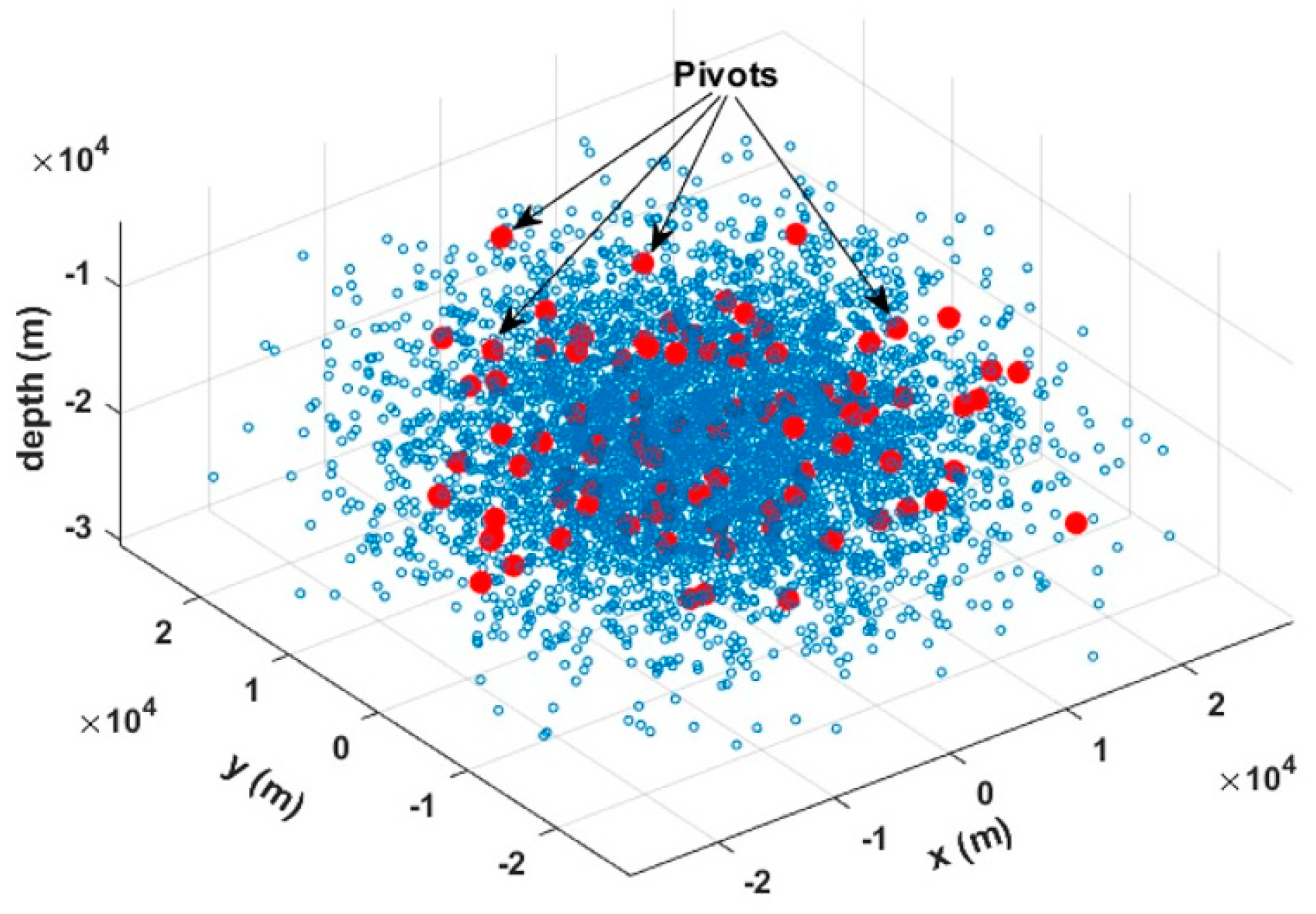
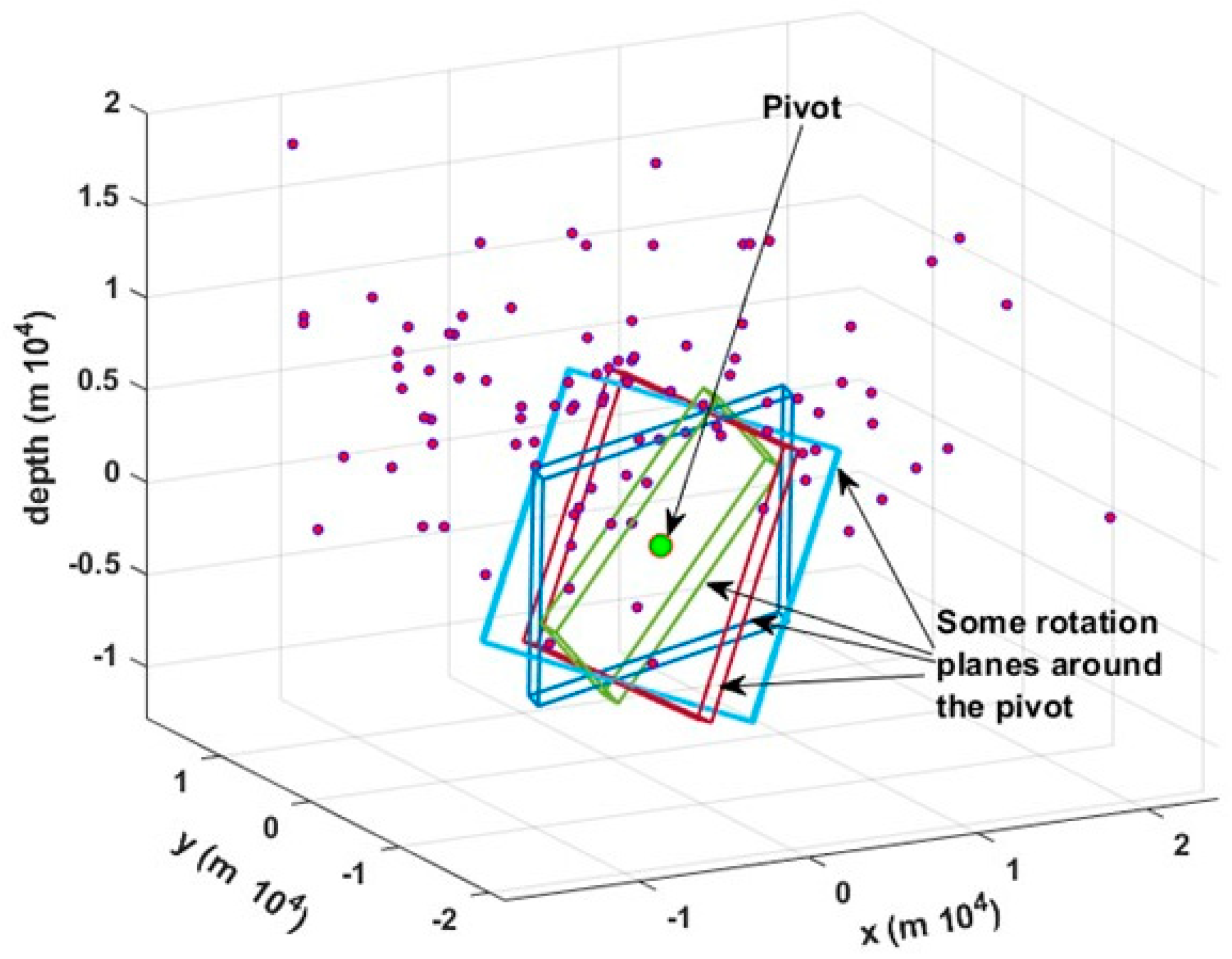
Step 1. The algorithm randomly extracts K (K ≪ N) pivot hypocenters (Pᵢ, i = 1, 2, …, K) from the N earthquake hypocenters (see Figure 1). It then translates the coordinate system so that the origin coincides with Pᵢ, which is assumed to be the rotation center for a hypothetical fault plane defined as a volume (V) (see Figure 2). Pivot points are selected using the Monte Carlo method [12,13] from the set of hypocenters, based on the knowledge that the fault plane must pass through them. Moreover, the K pivots follow the density distribution of the N hypocenters and are primarily located in regions with a higher probability of constituting a fault plane. This approach accelerates the search process and ensures that many pivots lie on the fault plane.

Step 2. We define a parallelepiped, the barycenter of which is a pivot hypocenter (cartesian coordinate 0,0,0), with thickness t (Figure 1) and volume V_j (Figure 2), such that the two dimensions, orthogonal to t, are much greater than t. The t value is assumed to be the mean error of the hypocenter localization (σ), but it can be increased to take into account slight deviations from the perfect planarity. Then, the algorithm counts the number of hypocenters which fall into the defined volume V_j.

Step 3. In this step, the reference system still centered on P_i, and the algorithm estimates, in all angular directions, the number (L) of hypocenters located in the V_j volumes, applying the two rotation matrices around the x and y axes. Note that in doing so, the algorithm works on two dimensions instead of on three dimensions, greatly speeding up the calculations.

For each P_i and for each rotation ($\vartheta$) around the x and ($\phi )$ y axes, the number of hypocenters L intercepted by the V_j volume is stored. This step consists of the maximization of the hypocenter number L in the V_j volumes as a function of the $\vartheta \mathrm{and} \phi$ angles and P_i:

$$max\left\{L\left[\left(V_j(P_i,{\vartheta }_r,{\phi }_q\right)\right]\right\}=>{\pi }_0\left(P_0,{\vartheta }_0,{\phi }_0\right)\left(i=\mathrm{1,2},\dots ,K;r=\mathrm{1,2}\dots R;q=\mathrm{1,2},\dots Q\right)$$

(1)

where $\vartheta \in \left[0°,180°\right],\phi \in$ [0°,180°] and R and Q represent the number of angular discretizations.

In this way, we individuate the plane ${\pi }_0$ that represents a fault plane found in the whole explored volume V = U(V_j).

Step 4. The following step consists of setting different fault dimensions (x, y) and the thickness (t) by increasing its initial value up to a few times σ. This method explores the parameters space (P, ϑ, φ,), even considering the thickness values. In particular, the study of the earthquake number belonging to the fault, as a function of the thickness t, gives information on the best t and on the goodness of the fault approximation.

At the end of the procedure, the solution is represented by a parallelepiped containing the maximum number of earthquake hypocenters.

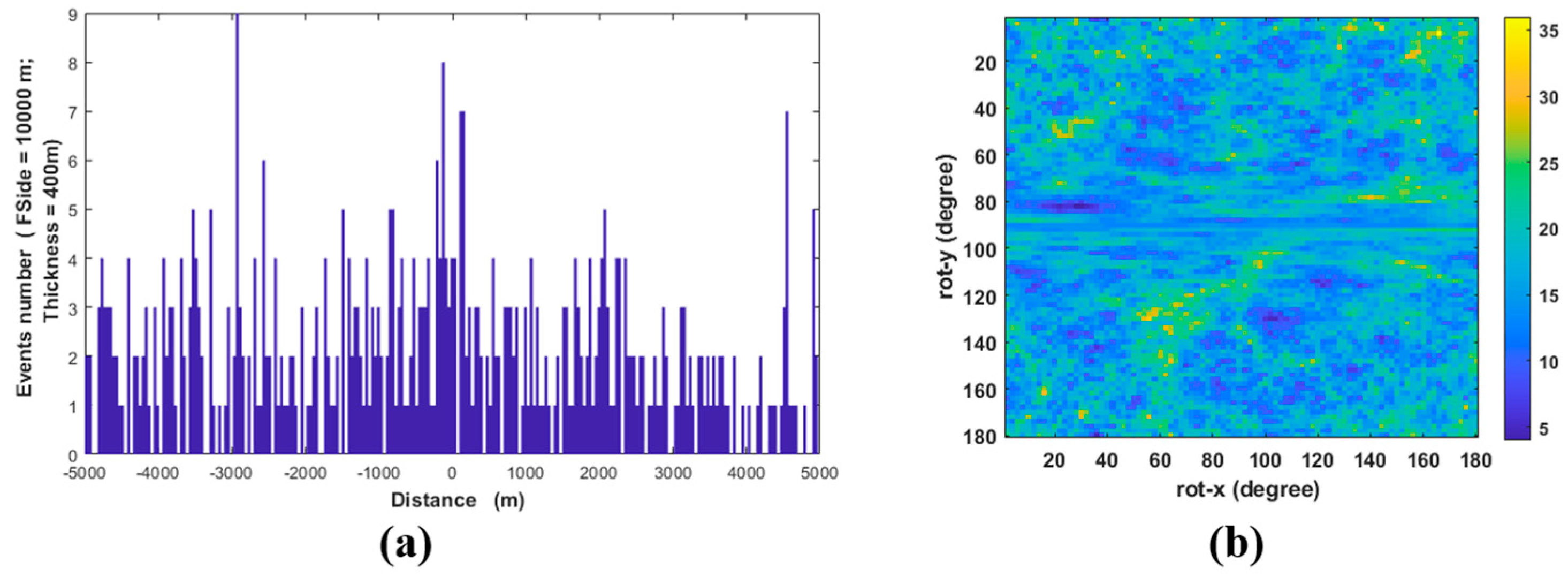
But how constrained is the solution? If we rotate the parallelepiped, how much does the earthquake count change? Figure 3a illustrates how the solution evolves as the reference system rotates around the two axes. A peaked solution indicates stability, whereas, for example, in a scenario without any faults (Figure 3a), the solution is completely unstable, showing multiple peaks and a lower number of counts. Furthermore, when a fault is present, it is expected that moving orthogonally away from the fault will result in a rapid decrease in the number of events. Specifically, if we translate the pivot that defines the solution parallelepiped orthogonally to the fault and construct a new parallelepiped (parallel to the solution), the number of events within the new parallelepiped will progressively decreaseas we move further away from the solution.

The algorithm was developed using Matlab R2024b adopting parallel computing.

3. Application to a Simulated Fault

To verify the reliability of our algorithm, we performed a blind test using two earthquake hypocenter distributions.

The first one was characterized by a random normal density distribution of 5000 hypocenters in a volume (x, y, z) of 40 × 40 × 20 km, without any planar event distributions. In order to identify the possible presence of a fault in that volume, we produced and analyzed a density function diagram (Figure 3a) and a conditional angular probability map (Figure 3b). After randomly selecting a certain number of hypocenters (300), the algorithm looks for areas with a greater density of epicenters and produces, as a result, a diagram like the ones shown in Figure 3a, where no significant density emerges.

In general, the absence of a fault is marked by a function which oscillates randomly without a clear trend and is characterized by various peaks with similar amplitudes (Figure 3a). Accordingly, the absence of a fault returns an angular conditional probability map (Figure 3b) without a clear pattern for any pairs of $\vartheta$ and φ angles. Figure 3b represents the results of all possible rotations of the explorer parallelepiped around the pivot with the maximum number of counted hypocenters. The absence of a well-defined nucleus highlights the clear lack of a fault plane.

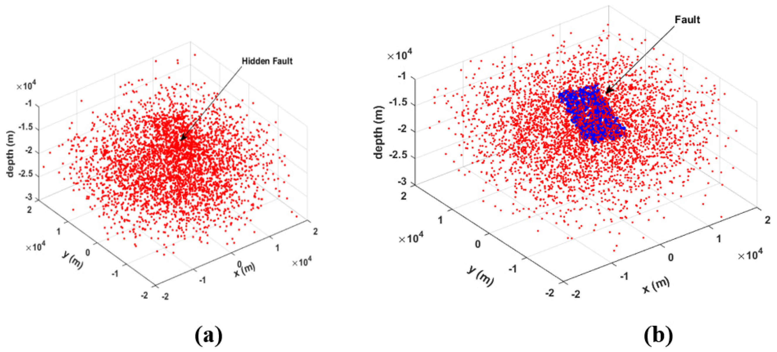
In the second case (Figure 4), the presence of a fault immersed in a normal random distribution of 5,000 hypocenters is simulated (Figure 4a). We added to the previous normal distribution a simulated fault made of 500 hypocenters with a random distribution in the x-y dimension (10 × 10 km) and a normal distribution, with variance of 200 m, in the z-dimension. The aligned earthquake distribution (i.e., the fault) initially on the z = 0 plane, is 35 degrees rotated with respect to the y-axis and 160 degrees rotated with respect to the x-axis. The algorithm converges towards the solution, which individuates the angles of the simulated fault.

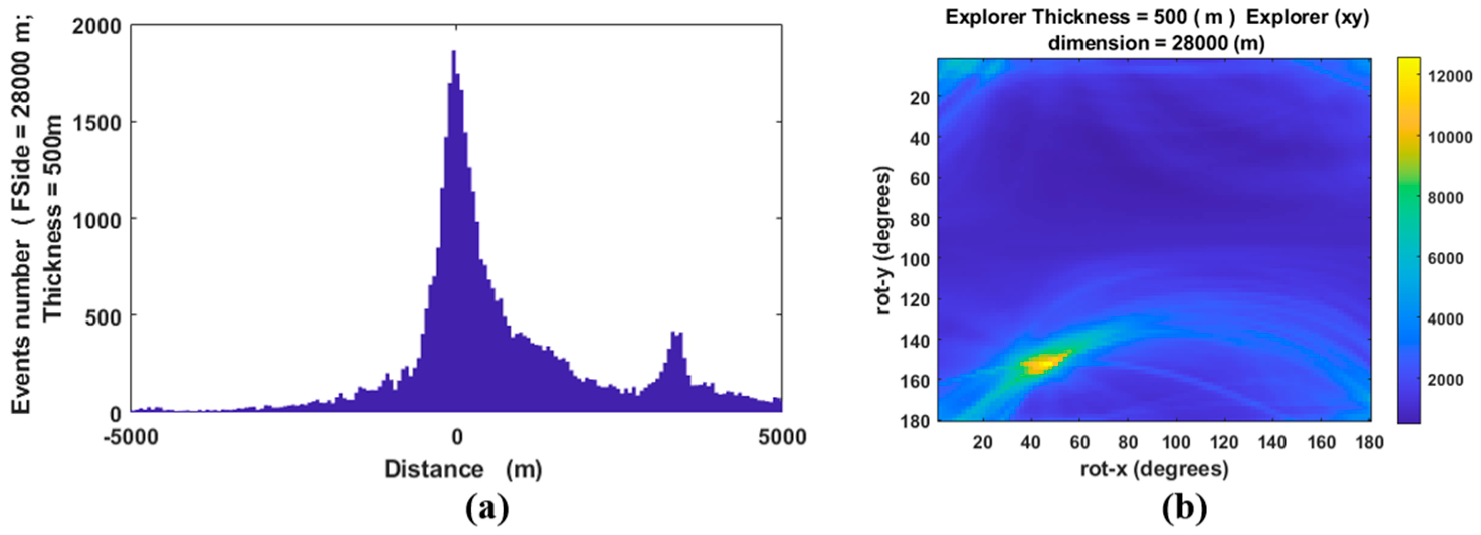
The results are shown in Figure 5a,b, where a clear density peak is shown which represents the presence of a well-defined fault. Figure 5b confirms the existence of a fault with a well-defined nucleus, which approximatively individuates the simulated fault angles.

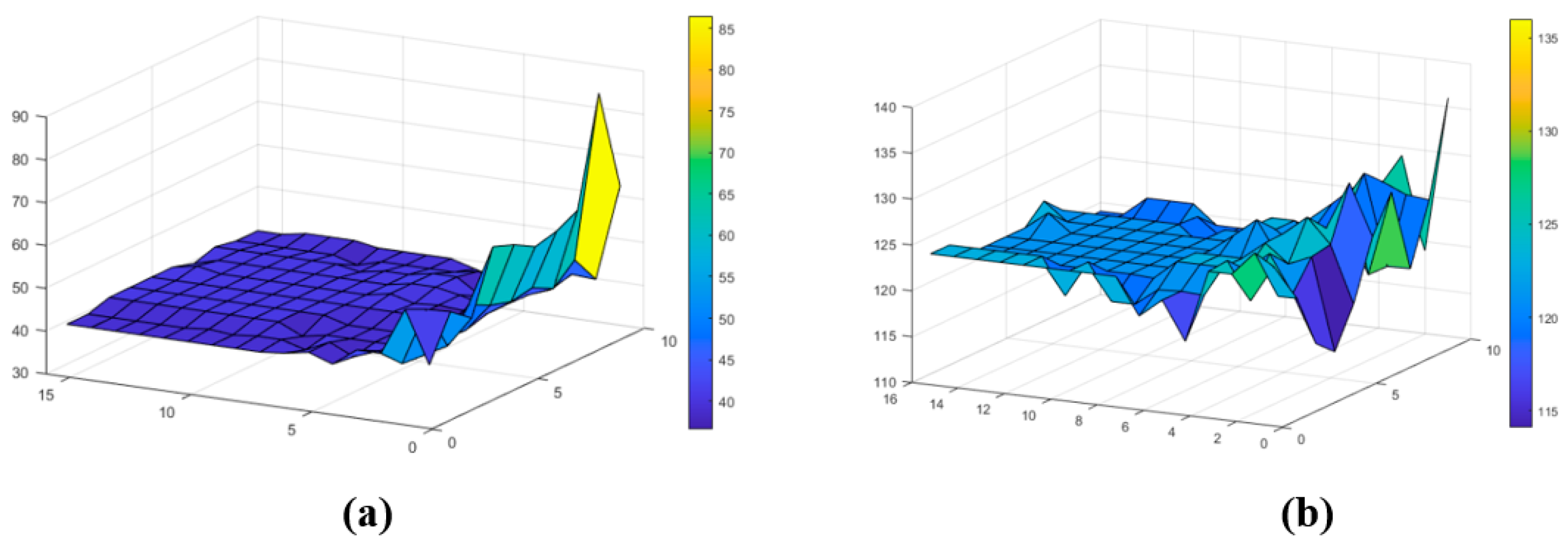
Figure 6a,b represent, respectively, the estimated dip and strike of the simulated fault as a function of the fault dimension and thickness. Both the dip and strike are individuated where the represented functions have stable behavior. In particular, the estimated dip value is approximately 40 degrees and the strike value about 124 degrees, which matches very well with the imposed simulated values.

4. Application to the L’Aquila 2009 Mw6.1 Seismic Sequence

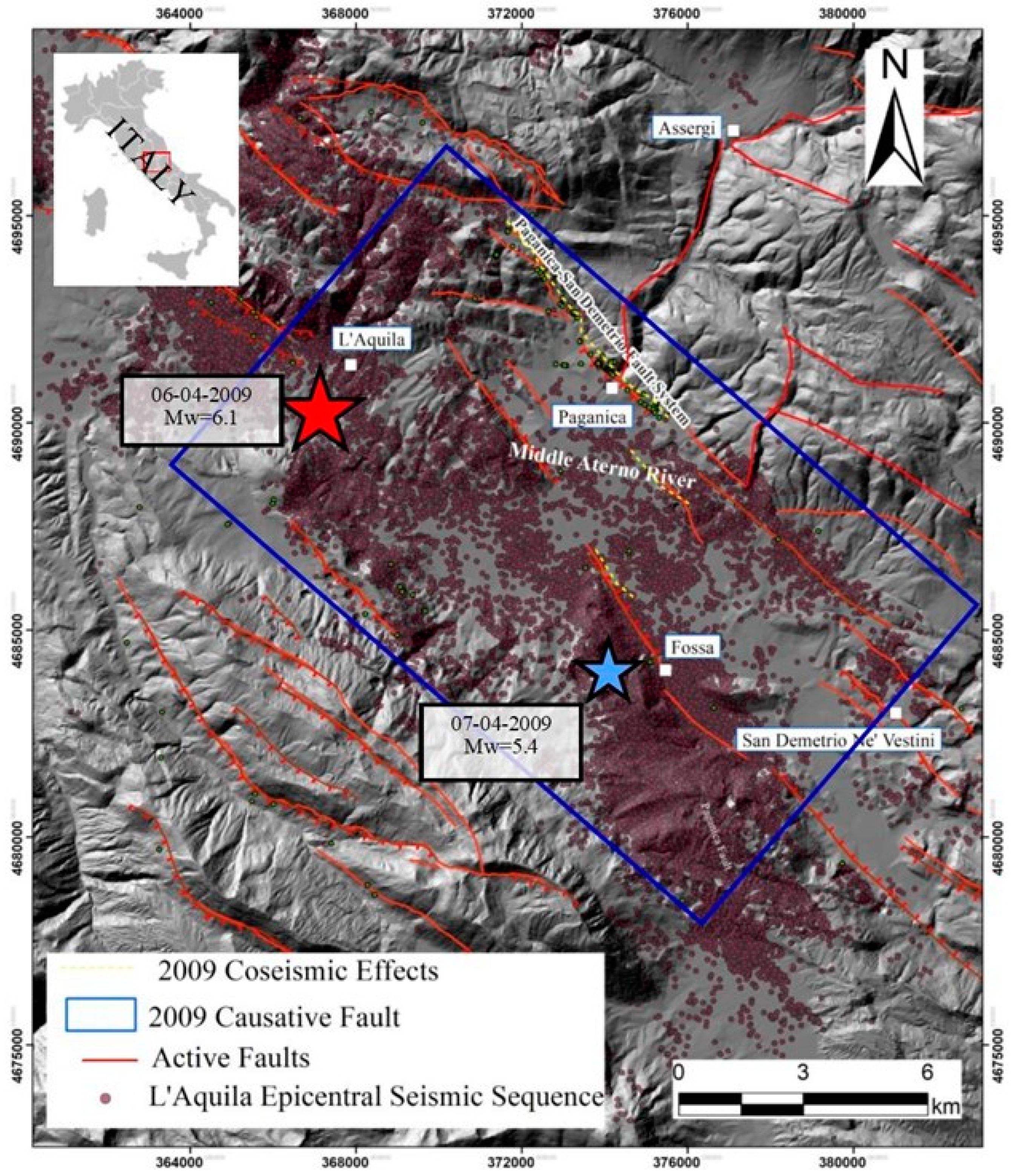
We tested the HYDE algorithm on a very well monitored real case: the seismogenic normal fault which caused the 2009 Mw6.1 L’Aquila earthquake in Central Italy.

The L’Aquila earthquake sequence fits the seismotectonic context of the area well: seismologic, geodetic, DInSar and geological data clearly indicate that the Paganica–San Demetrio fault system (PSDFS) is the seismogenic fault of the Mw6.1 6 April 2009 main shock [14,15,16,17,18].

The focal mechanism indicates a fault plane with an N140° direction and dipping about 45–50° to the SW [19], in agreement with the regional SW–NE extensional stress field active in the region. The seismogenic fault responsible for the 2009 l’Aquila main shock coincides with the surface expression of the PSDFS which bounds the northeast of the Aterno River valley (Figure 7). It shows complex surface expression, with several synthetic and antithetic splays affecting the Quaternary basin continental deposits [20,21,22,23,24].

Before the 2009 earthquake, the geometry and activity of the PSDFS was only roughly known. It was mapped as an uncertain or buried fault [21,22,25,26].

During the 6 April main shock, this fault created a limited coseismic surface displacement observed for a total length greater than 3 km, consisting of a complex set of small scarps (up to 0.10–0.15 m high) and open cracks with a direction in agreement with the focal mechanism of the main seismic events.

Other discontinuous breaks occurred, with a trend ranging from N120° to N170°, to the north and south of the main alignment of ruptures. In this case, the length of the surface faulting may exceed 6 km [18,27].

Figure 7. Location map of the 2009 L’Aquila main shocks: stars indicate M > 5.0. The red lines are the main active faults extracted from Galadini and Galli [28] and the Ithaca catalog [24,29]. The blue box is the projection to the surface of the ~19 km long 2009 main shock causative fault according to several investigators ([30] and references therein). The red points are the 2009 l’Aquila seismic sequence relocated by [31]. The yellow dashed lines are the 2009 coseismic ruptures from [18].

Figure 7. Location map of the 2009 L’Aquila main shocks: stars indicate M > 5.0. The red lines are the main active faults extracted from Galadini and Galli [28] and the Ithaca catalog [24,29]. The blue box is the projection to the surface of the ~19 km long 2009 main shock causative fault according to several investigators ([30] and references therein). The red points are the 2009 l’Aquila seismic sequence relocated by [31]. The yellow dashed lines are the 2009 coseismic ruptures from [18].

Other cracks are detected along the antithetic structures of Bazzano and Monticchio–Fossa. The seismicity distribution of the 2009 L’Aquila foreshock and aftershock sequence indicates that the epicentral area has a length of 50 km along the NW-SE direction defined by a right step en-echelon fault system, with earthquakes mostly confined below 2 km [14,15,31]. This suggests that only minor slips took place on the shallower portion of the fault, in agreement with surface observations.

The 3D architecture of the Mw6.1 L’Aquila main shock causative fault has been accurately described by [31] by using a high-quality earthquake catalog composed of about 64,000 foreshocks and aftershocks that occurred within the first year, processed through automatic procedures. In particular, high-precision foreshock and aftershock locations delineated an about 16–18 km long fault (the Paganica fault), showing an almost planar geometry. The aftershock distribution around the main slipping plane varies from small (about 300 m) close to the main shock nucleation to large (about 1.5 km) at the south-eastern termination of the fault [32]. This along-strike change in fault zone thickness has been related to the heterogenous coseismic slip distribution along the fault and to an increase in fault geometrical complexity at the south-eastern fault termination [32].

The heterogeneous 2009 coseismic rupture is well documented [33,34]. The main shock nucleated at about an 8 km depth. At first, the rupture propagated up-dip with the coseismic slip located 2 km up-dip from the main shock hypocenter; then, it continued along the strike direction to the SE portion of the fault and at shallower depths [35].

4.1. Dataset Description

Here, we used a very detailed earthquake catalog computed by [31] by processing continuous seismic data recorded at a very dense seismic network of 60 stations operating for 9 months after the Mw 6.1 main shock. The complete catalog is composed of about 64,000 precisely located foreshocks and aftershocks, spanning from January to December 2009. It was processed by combining an accurate automatic picking procedure for P- and S-waves [36], together with cross-correlation and double-difference location methods [37], reaching a completeness magnitude (i.e., the minimum magnitude above which all of the events occurring in a study area can be reliably detected and located [38]) equal to 0.7, which corresponds to a source dimension of ~50 m based on a circular crack model using a 3 MPa stress drop. The earthquake relative location errors are in the range of a few meters to tens of meters (i.e., the error ellipsoids obtained at the 95% confidence level for 200 bootstrap samples show median values of the distribution along the major/minor horizontal and vertical directions of 24, 15 and 27 m; see [39] for details). These errors are comparable to the spatial dimension of the earthquakes themselves, allowing us to image the internal structure of the fault zone down to the tens of meters scale.

For this work, we use the complete large-scale catalog, relative to the L’Aquila Mw6.1 main shock, differently from what is shown in [35] where the authors choose earthquakes occurring within 6 km (±3 km) from the L’Aquila fault plane, modeled by inverting strong motion, GPS and DInSAR data. That plane is 20 km long in the N133°E striking direction and dips 54° to the SW, intersecting the main shock hypocenter. Their resulting catalog is made of ~19k foreshocks and aftershocks. Further details on this catalog are described in [32], which deals with the accurate description of the L’Aquila 2009 fault zone structure and damage zone and its implication for earthquake rupture evolution. Our large-scale and complete earthquake catalog represents a perfect test-case to verify the ability of the HYDE algorithm to retrieve both the large- and small-scale complexities of the activated faults.

4.2. Application to L’Aquila Dataset

We used the HYDE algorithm to define the parameters (strike, dip, length and fault zone thickness) of the Mw6.1 L’Aquila seismogenic fault, which generated the Mww6.1 mainshock and the aftershock sequence.

Following the algorithm steps, we first used the earthquake distribution to identify a set of 1000 pivot hypocenters, assumed to be the rotation centers of the fault plane. We conducted different tests, both changing the possible length of the fault plane from 4 km to 32 km (with a 4 km sampling rate) and allowing the fault zone thickness to vary from 100 m to 800 m (with a 100 m sampling rate), according to previous studies [32]. The initial chosen thickness of 100 m takes into account the order of the localization error, which implies a flat fault. Increasing fault thickness values will comprise non-planar faults, as is often observed in real cases.

Figure 8 shows the results for a fault zone thickness fixed at 500 m. The results (Figure 8a) show a clear density peak, which represents the presence of a well-defined fault. Figure 8b confirms the existence of a fault with a well-defined nucleus, which approximatively individuates the estimated dip and strike of the main L’Aquila fault.

In particular, i Figure 9a,b presents, respectively, the estimated dip and strike of the L’Aquila fault as a function of the fault dimension and thickness. Both fault dip and strike are individuated where the represented functions have stable behavior. In particular, the estimated dip value is approximately 52 degrees and the strike value about 36 degrees, which matches the estimated values by [32,35,36] well.

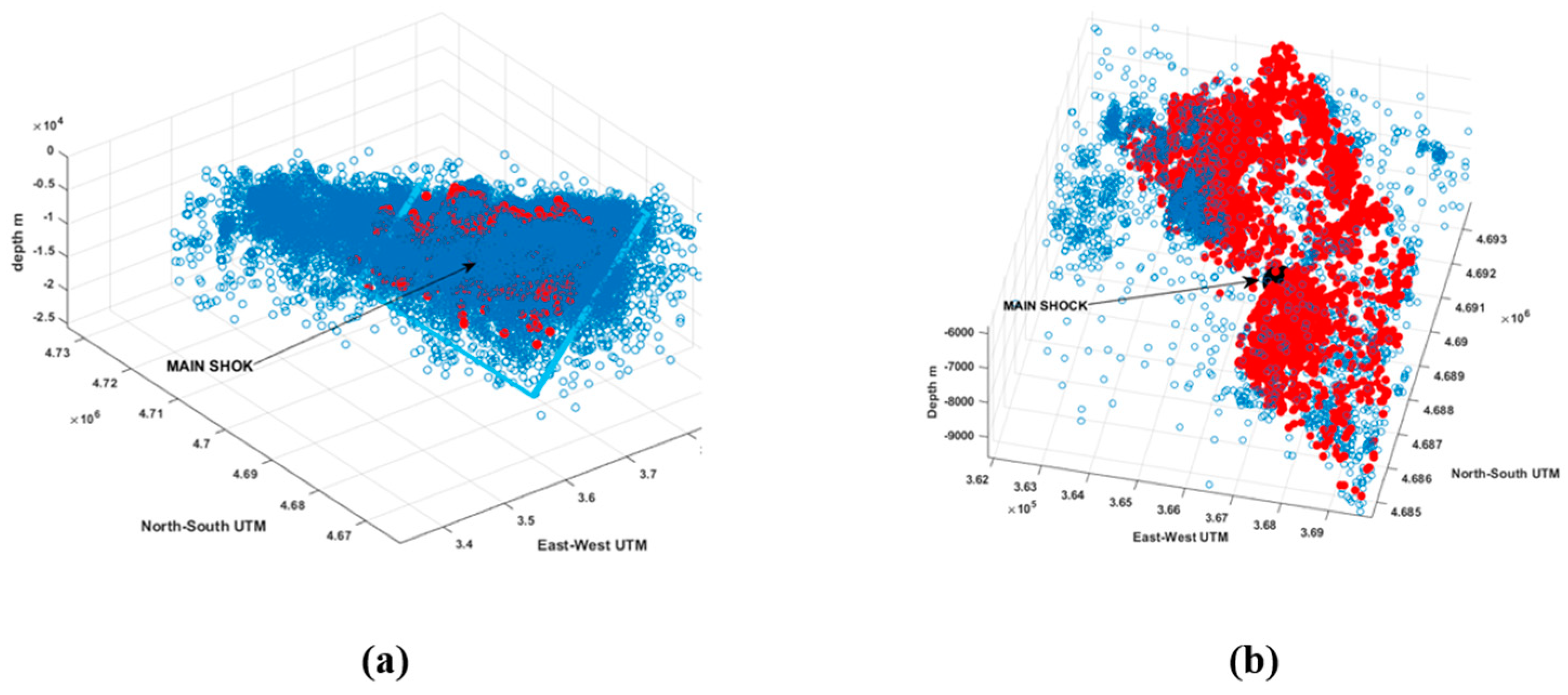
For a fault with thickness of 500 m and a length of 24,000 m, we obtain the solution shown in Figure 10, where it is clear that the main shock is contained in the parallelepiped, which individuates the main fault plane. This is a very important result considering that the algorithm does not use constraints, for example, ones based on the main shock location to drive the solution. The main shock does not affect the exploration of spatial parameters at all. The algorithm does not impose any constraints forcing the fault plane to pass through the main shock. Moreover, the structure responsible for the main shock is generally the same as the one that triggers the aftershocks. Other substructures—whether parallel or even orthogonal to the main fault—are usually characterized by a lower number of earthquakes and are initially disregarded by the algorithm. This indicates that our algorithm is a very useful and reliable tool.

5. Discussion

We designed and developed an algorithm named HYDE, able to estimate the geometry (size, depth, dip and strike angles) of fault planes using the hypocenter locations of main earthquakes and the associated aftershocks, even where the seismogenic sources are fragmented.

Our HYDE algorithm is still capable of accurately identifying fault parameters even when the fault geometry is highly non-planar or complex. In cases of fault segmentation, when there are multiple contiguous planar faults with appreciably different strikes and/or dips, the algorithm will first identify the fault segment that contains the largest number of earthquakes. Then, by excluding the earthquakes belonging to this primary fault, the algorithm searches for the next fault cluster, and so on, providing the respective strike, dip and mean location for each identified fault.

In cases where fault substructures are orthogonal to the main fault, the algorithm ignores them (along with the associated earthquakes) because they are assigned a weight of zero, as they lie outside the explorer parallelepiped that defines the main fault.

When the fault structure takes the form of a cylindrical surface sector, we need to express the earthquake locations in cylindrical coordinates. In this system, the distance from the curved fault surface corresponds to the r-coordinate of the 3D reference system. The analog of a parallelepiped in Cartesian coordinates is a volume contained between two concentric sectors. Many pivots will be attracted to this sector, as in the planar fault case; however, we now need to explore two additional parameters: the cylindrical curvature and the rotation of the symmetry axis.

In this scenario, the computing time increases by a factor that depends on the number of discretized curvature values multiplied by the number of discretized rotations for the symmetry axis. For the 2009 L’Aquila seismic sequence, involving approximately 64,000 earthquakes analyzed using Cartesian coordinates, we used 1000 pivots to achieve comprehensive coverage of the parameter space. When run on an Intel i7 PC with 16 cores, the computing time was approximately 10 days.

The number of pivots to choose depends on the ratio between the number of earthquakes associated with the fault and the number of localization points outside the defined parallelepiped. However, assuming we have 1000 positive events (within the parallelepiped) and 9000 negative events, the probability of obtaining a null extraction from the fault is approximately 10⁻⁵, a very low probability. Consequently, the random selection of pivots will likely include around 100 pivots on the fault, statistically distributed according to the density of earthquake hypocenters. In our case (see Figure 8b), about 15,000 to 20,000 earthquakes are associated with the fault, which is a significant fraction of the 64,000 events considered. Using 200 pivots yielded practically the same result. Obviously, determining the optimal number of pivots must be evaluated on a case-by-case basis; however, the fault tends to act as an attractor for the pivots. Different considerations are necessary for substructures with fewer events. In these cases, it is advisable to first isolate the involved volume and then rerun the code—in that subspace, the same considerations still apply.

Our algorithm is particularly useful where the earthquake intensity is not so high that the radiation pattern can be easily determined, as often happens for most aftershock sequences or in volcanic areas, where the percentage of earthquakes for which the radiation pattern can be defined is very low. One of the advantages of the proposed method is that it does not require focal mechanisms at all. The method relies solely on the earthquake locations and is particularly suited for exploring data such as tectono-volcanic earthquakes, which are difficult to analyze using other methods due to their typically 3D distribution, low magnitude and obscured alignments. As shown in Figure 4a, the classical method requires first identifying the fault (Figure 4b, blue points), then selecting a subset of data where alignment may be evident, and finally, estimating the probable fault structure. In contrast, our method eliminates the need to select a data subset and quickly arrives at the solution. Notably, the computation time for 5000 events and 50 pivots is only tens of minutes when using an I7 PC with 16 cores.

Assuming that most of the earthquakes are clustered on fault planes, the algorithm finds the principal fault using a density-driven search. It works as a Monte Carlo method applied to a subspace constrained by the pivot hypocenters.

The strength of the proposed method is based on the use of a very robust norm such that when earthquakes belong to the explorer parallelepiped, they are assigned a weight 1; if not, the weight is zero, and this avoids the well-known problem of outliers in the statistical analyses. Conversely, the capability to explore the whole parameter space avoids the trapping of the solution into a local minimum. The algorithm’s ease of use, lies in the use of a distance which is, due to rotation, derived from a single variable from the plane.

We tested our algorithm on a synthetic dataset and on the real case of the L’Aquila 2009 seismic sequence. The obtained results for both study cases show that HYDE is a very suitable and reliable tool that is able to identify the main fault plane even in the presence of many fault segment substructures. In particular, for the real L’Aquila case, we identified, using our algorithm, that the geometry of the main fault plane is in good agreement with the independently calculated focal mechanism [32]. This validates our results, paving the way to several applications of the proposed method where focal mechanisms are not available or not well constrained to reduce uncertainties.

Moreover, regarding the L’Aquila earthquake sequence, we performed a search using 1000 pivots to obtain stable fault parameters, but a search with only 200 pivots already gave us the same solution. This depends on the nature of the clustering of the earthquakes on the fault plane, which attracts the explorers to the right subspace, considerably reducing the algorithm run time. The results of the application of our algorithm on both the synthetic and the real L’Aquila case show that HYDE is able to quickly individuate the seismogenic fault planes even for complex fault geometry. Moreover, when refined seismic catalogs are not available, it is still possible to successfully use our algorithm, calibrating the thickness of the explorer parallelepiped according to the localization error magnitude. Note that the program includes a search for substructures of any dimension, simply extracting data in a local subspace. Future improvements to the HYDE algorithm may include time constraints to study the hypocenter’s temporal evolution in order to explore the kinematics of the fault plains. Once the thickness and dimensions of the seismogenic fault have been estimated, it is possible to extract from the entire earthquake dataset those events associated with the fault identified by the explorer parallelepiped in order to track the temporal evolution of the ruptures.

The obtained results and their validation, by means of comparison with independent studies, pave the way to several applications.

The HYDE algorithm may be particularly useful where the earthquake intensity is not so high that the radiation pattern can be easily determined, as often happens for most aftershock sequences or in volcanic areas, where the percentage of earthquakes for which the radiation pattern can be defined is very low. Thus, when earthquake properties, such as the magnitude and focal mechanism, are difficult to determine, the HYDE algorithm can still provide seismotectonic information. We can generalize that the HYDE algorithm can be useful as an alternative or complementary tool to other investigation methods to reduce the uncertainties inherent in each method. In this regard, it should be stressed that fault parameter estimates are also affected by uncertainties when using approaches other than focal mechanisms. Statistical approaches such as Bayesian estimation, as well as numerical modeling methods, are useful to provide an understanding of geological processes and kinematic models [39,40,41]. However, these approaches require a priori information that is not always available, and the results depend on the boundary conditions and the accuracy of the many input parameters. Instead, our algorithm requires only the coordinates of the hypocenters as input data and does not require any constraints or boundary conditions, but does not provide slip angles. As a consequence, the size dip and strike obtained by HYDE may also be used as input parameters to reduce the uncertainties in slip estimates obtained by Bayesian estimation and numerical modeling methods. The value of the proposed algorithm becomes even more evident in terms of its application in the various fields in which knowledge of fault parameters is fundamental. Indeed, accurate knowledge of active fault geometries is also essential for earthquake ground motion evaluation, which, in turn, is crucial for seismic hazard assessments [41]. Thus, the HYDE algorithm may also be useful for subsoil characterization in the framework of performance-based earthquake engineering, reducing uncertainties in seismic fragility estimates [42,43,44].

General approaches to estimating fault strike and dip require collapsing the earthquake data onto a flat plane. For example, using the double-difference method, the data are transformed into a collinear dataset and then inverted using an L₁ or L₂ norm or another more robust norm. Other algorithms—such as the planar best-fitting method [45], which is based on the inertia tensor—are, like the double-difference method [37], heavily influenced by earthquakes located outside the fault zone. This trade-off is typically managed by carefully selecting the dataset.

Our algorithm, however, automatically ignores all earthquakes outside the fault zone and can estimate the fault parameters without any prior data selection. This makes it particularly efficient and useful when rapid estimation of an active fault’s strike, dip and mean location is needed. In particular, for the 2009 L’Aquila seismic sequence, we used the complete earthquake dataset to run our HYDE algorithm and determine the main fault plane parameters, in contrast to [32], who used a selection of hypocenters near the main fault to delineate its structure.

Moreover, when refined seismic catalogs are not available, it is still possible to successfully use our algorithm, calibrating the thickness of the explorer parallelepiped according to the localization error magnitude.

There are very few limitations when using the HYDE algorithm. However, when earthquake hypocenters are distributed on a curved structure, the algorithm will typically identify the fault in the area of lower curvature where event density is highest. Currently, we are unable to estimate the fault parameters for a curved structure or determine the location, strike and depth of the main shock if it occurs far from the lower-curvature region. Moreover, in the case of a highly segmented fault—i.e., a sequence of small segments of varying lengths separated by step-overs—the algorithm will identify a fault plane that encompasses all segments, with dip and strike parameters corresponding to the principal alignment, thereby providing only an approximate result. Another limitation is that when defining the initial parameters for the exploratory parallelepiped, we must choose values close to the actual approximate size of the target fault; otherwise, the fault parameter space becomes too broad, leading to excessively long computation times.

6. Conclusions

In conclusion, we designed and developed the HYDE algorithm to estimate the geometry (size, depth, dip and strike angles) of fault planes using the hypocenter locations of earthquakes. Assuming that most earthquakes are clustered on fault planes, the algorithm identifies the principal fault using a density-driven search even in complex fault geometries.

The effectiveness of HYDE in rapidly and accurately identifying seismogenic fault planes makes it a useful tool for seismotectonic studies when other methods are not applicable, or in a complementary manner to reduce uncertainties. The applicability of the algorithm in real cases is extremely straightforward when a dataset containing only the 3D locations of the earthquakes is available. In the L’Aquila 2019 case, which involved a seismic sequence of 70,000 events, we tested the algorithm using 1000 pivots (rotation centers) on a 16-core PC, achieving a runtime of approximately one week. We emphasize that we obtained the same result using only 200 pivots in a high-density earthquake area, with a runtime of just 2 days, on an Intel i7 16-core PC. This capability is fundamental for risk mitigation, as it enables us to accurately and rapidly define the seismogenic area and implement appropriate security, civil protection measures and mitigation strategies. The key is to have many computed hypocenters available as quickly as possible.

Future enhancements to the algorithm could provide even greater insights into the kinematics and temporal evolution of fault planes, further broadening its scope of application.