Research on Bearing Remaining Useful Life Prediction Method Based on Double Bidirectional Long Short-Term Memory

Abstract

The predictive capability of traditional bearing remaining useful life (RUL) prediction models is insufficient, and the prediction networks lack universality, leading to unsatisfactory results in predicting the RUL of bearings, which leads to untimely maintenance decisions and significant economic losses. In order to solve this problem, this study employs Discrete Wavelet Transform (DWT) to denoise vibration signals and extract multi-domain features; the weighted averages of monotonicity, predictability, trendability, and robustness indicators are first ranked for selecting sensitive feature subsets as inputs for RUL prediction, feature fusion is conducted using the Kernel Principal Component Analysis (KPCA) method to obtain the health index (HI) of the bearing, and the failure threshold of the signal is determined based on the 3-sigma principle. An RUL prediction model, which combines Double Bidirectional Long Short-Term Memory (DBiLSTM) with attention mechanism (A-DBiLSTM), is then developed, and the Bayesian approach is used to adaptively search for network hyperparameters. Experiments were conducted using the PHM2012 dataset and the XJTU-SY dataset; the results indicate that the proposed RUL prediction model demonstrates higher predictive performance, exhibits satisfactory performance across different datasets, and possesses good generalization capability and applicability. This method further enhances the predictive capability of bearing RUL estimation.

1. Introduction

Rolling bearings are essential components that provide support for rotating shafts. They are widely used in various rotating machinery systems [1]. The unexpected failures of bearings can increase the maintenance costs and downtime, leading to significant economic losses [2]. By predicting the Remaining Useful Life (RUL), maintenance schedules and part replacements can be proactively planned. Consequently, the accurate RUL prediction for bearings is crucial for ensuring machine health, reducing costs, and optimizing production [3]. When data-driven methods are adopted to predict the bearing RUL, the prediction performance highly depends on the selection of degradation-sensitive features and the prediction model type [4]. Many studies used single feature indicators as degradation features for bearings, such as the root mean square (RMS) [5], kurtosis [6], and spectral kurtosis [7]. However, these single indicators often fail to comprehensively reflect the trend of the bearing degradation. Thus, other studies considered multiple features as degradation-sensitive features of bearings and inputted all these features into RUL models. The latter processes these features, yielding accurate prediction results [8,9]. Many models for RUL prediction exist, such as shallow machine learning (ML) models [10], Wiener processes [11,12], Bayesian methods [13,14], and machine learning models (e.g., extreme learning machines (ELMs) [15,16]). In addition, artificial neural networks [17,18], support vector machine (SVM) [19], independent component analysis (kurtosis, negentropy) [20], convolutional neural networks (CNNs) [21], deep belief networks [22], recurrent neural networks (RNNs) [23], Long Short-Term Memory (LSTM) networks [24], gated recurrent units (GRUs) [25,26], graph neural networks (GNNs) [27], and hybrid models [28] are widely used.

Shang et al. [29] processed the original vibration signals through Wavelet Packet Transform (WPT) and Complete Ensemble Empirical Mode Decomposition (CEEMD). Matania et al. [30] investigated the state-of-the-art methods for bearing vibration signal processing and conducted code demonstrations using software. Randall et al. [31] studied the vibration signal-based condition monitoring, and various monitoring methods for different vibration states have been listed. Wu et al. [32] applied Fast Fourier Transform (FFT) to convert the original time-domain data of bearing faults into the frequency domain, utilized the Particle Swarm Optimization (PSO) algorithm to optimize the parameters of the Support Vector Machine (SVM), and conducted denoising processing on the vibration signals. Li et al. [33] proposed a degradation feature fusion model that incorporates time-domain, frequency-domain, and time-frequency-domain features into monotonic curves and adopted state-space estimators to predict the bearing RUL. Yang et al. [34] predicted bearing RUL by determining precise thresholds. This was based on the incorporation of the Mahalanobis distance into an improved independent component analysis method. Kumar et al. [35] used signal entropy to represent degradation features and applied hybrid metrics to determine bearing failure thresholds. Qi et al. [36] determined bearing failure thresholds by filtering signals in different frequency bands and extracting various advanced entropy features and sparsity measures. Li et al. [37] predicted bearing RUL by combining CNN with Bidirectional LSTM (BiLSTM). Lu et al. [38] proposed a hybrid prediction method combining the digital twin technology with LSTM networks. This method predicts the bearing RUL based on the use of physical and virtual data. Li et al. [39] predicted bearing RUL by first fileting the underlying signal using a particle filtering algorithm, then combining CNN and LSTM networks. Fan et al. [40] predicted bearing RUL by first extracting bearing degradation features using BiLSTM, then combining them with a Transformer. Wang et al. [41] predicted bearing RUL by extracting 13 multi-domain features of bearings and using an LSTM network. Gan et al. [42] developed a model integrating gated convolution and temporal convolution. Zhao et al. [43] combined vibration signals and mechanism models and used BiLSTM networks. Rathore et al. [44] used stacked BiLSTM and attention mechanism. Shang et al. [45] employed LSTM networks and bidirectional GRUs. Jiang et al. [46] proposed a dual-channel convolutional network, which incorporates the Transformer algorithm.

In the aforementioned literature, although many scholars have employed LSTM or BilSTM for predicting the RUL of bearings, the predictive performance and applicability of the models still need to be enhanced. In order to address the aforementioned issues, the paper is structured into the following aspects:

Section 1 describes the research background, current research status, and research significance of the studied content, followed by a summary.

In Section 2, this paper employs the Discrete Wavelet Transform (DWT) for denoising the vibration signal, to obtain a pure signal. Features are extracted from the time domain, frequency domain, and time-frequency domain, the sensitivity of each feature is then evaluated using monotonicity, trendability, predictability, and robustness indicators, and the Kernel Principal Component Analysis (KPCA) is utilized for feature fusion and uses the fused value as the health indicator (HI) for the bearing. This chapter provides the data foundation for predicting the remaining useful life of bearings.

In Section 3, the method combines the application of a Doubled Bidirectional Long Short-Term Memory (DBiLSTM) network with an attention mechanism (A-DBiLSTM), describing the principles of the DBiLSTM network and the attention mechanism network, adaptively searching for network hyperparameters using Bayesian optimization algorithm. By using the 3σ (Three Sigma) method and combining the health indicator (HI) obtained in the second chapter, the health stage and failure stage throughout the entire life cycle of the bearing can be determined, and the process for estimating the remaining useful life of bearings can be outlined. This chapter outlines the complete process for predicting the remaining useful life of bearings.

In Section 4, experimental validation is conducted on the remaining useful life prediction method for bearings proposed in the third chapter, the proposed remaining useful life prediction method is compared with other methods, the obtained prediction results are analyzed, and its performance is evaluated using evaluation metrics.

In Section 5, the main conclusions are drawn, and a summary is provided.

The overall technical route is shown in Figure 1.

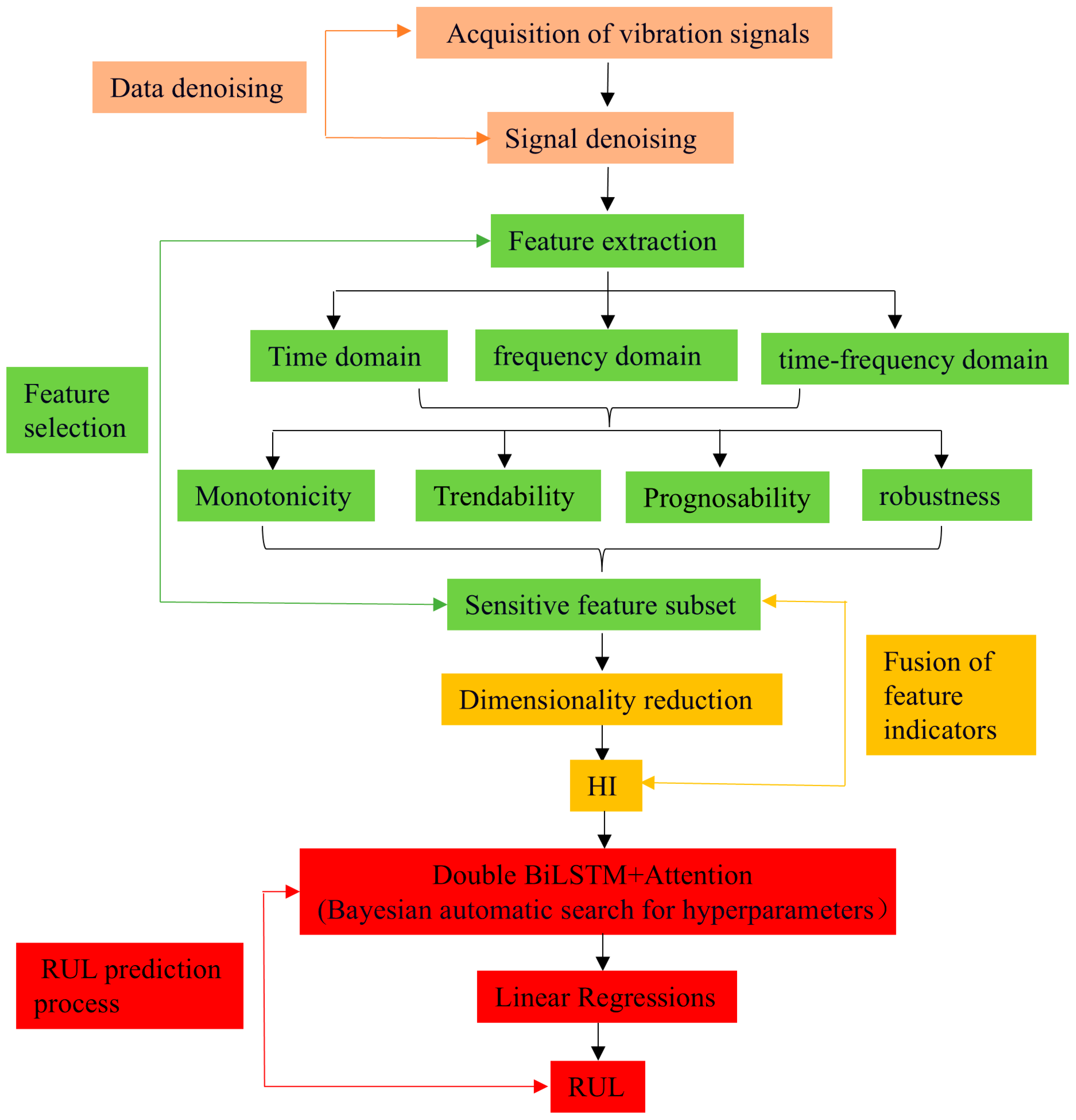
2. Vibration Signal Processing Methods

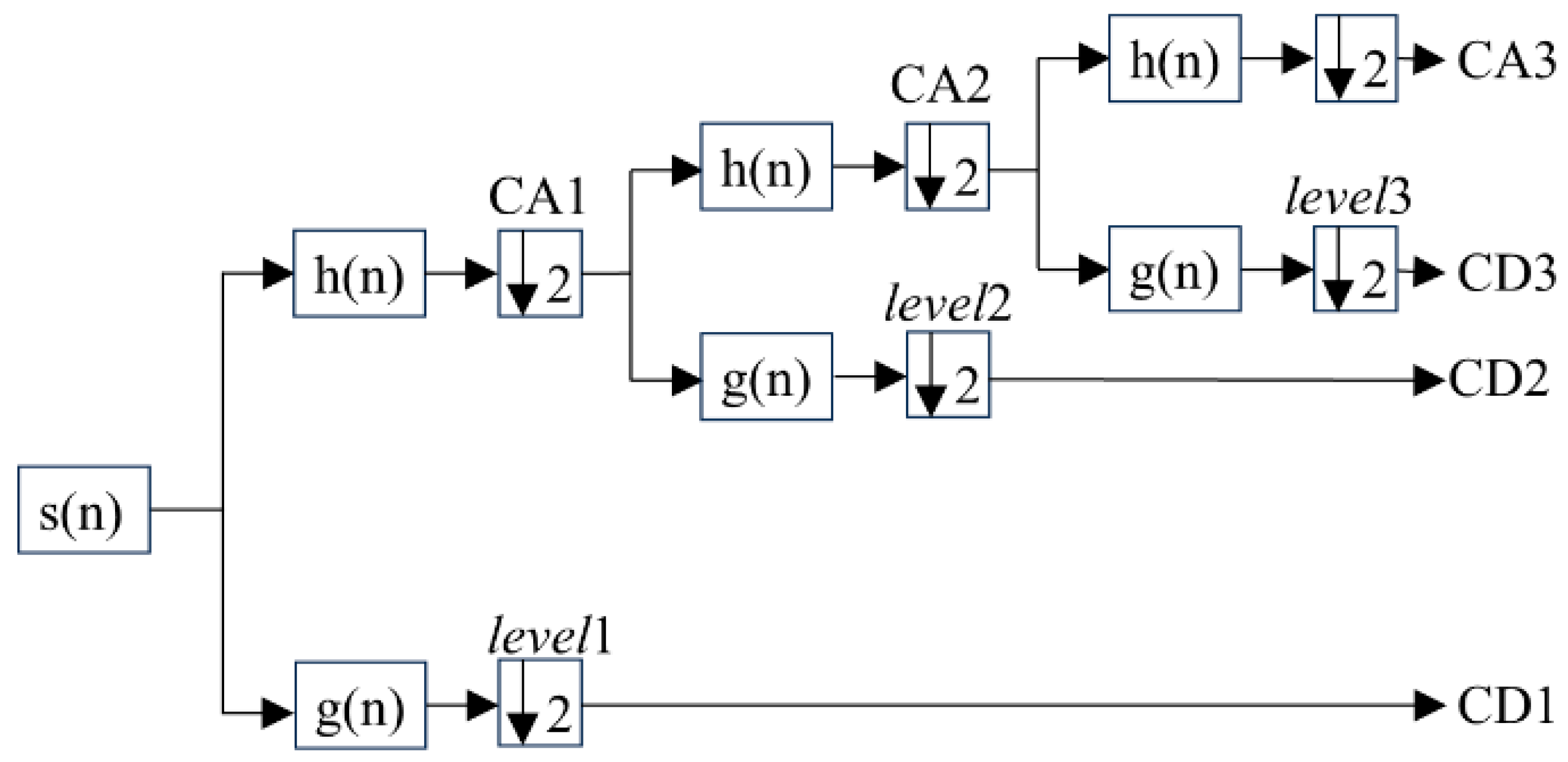
2.1. Signal Denoising Processing Methods

Denoising is performed using DWT, as shown in Figure 2. Three-level decomposition is first conducted using the Daubechies 3 mother wavelet, and denoising is then performed by soft thresholding. This results in dividing the vibration signal s(n) into two frequency sub-bands. s(n) is first passed through a low-pass filter h(n) and a high-pass filter g(n), followed by 2-fold down-sampling. This process converts it into approximation component CA1 and detail component CD1. Through multi-frequency analysis, the detail components CD and approximation components CA of the three levels of decomposition are determined as [44]:

$$\mathrm{s}\left(\mathrm{n}\right)=CD1+CD2+CD3+CA3$$

(1)

The soft thresholding is expressed as [46]:

$${\delta }_s(x,\lambda )=\left\{\begin{array}{c}\mathrm{sgn}(x)(x-\lambda )\left|x\right|\ge \lambda \\ 0\left|x\right|\le \lambda \end{array}\right.$$

(2)

where λ is the threshold, and x is the denoised detail coefficient. λ is computed as $\lambda =\sqrt{2{\log }_{e}M}$, where M is the number of data points.

2.2. Multi-Domain Feature Extraction and Sensitive Feature Selection

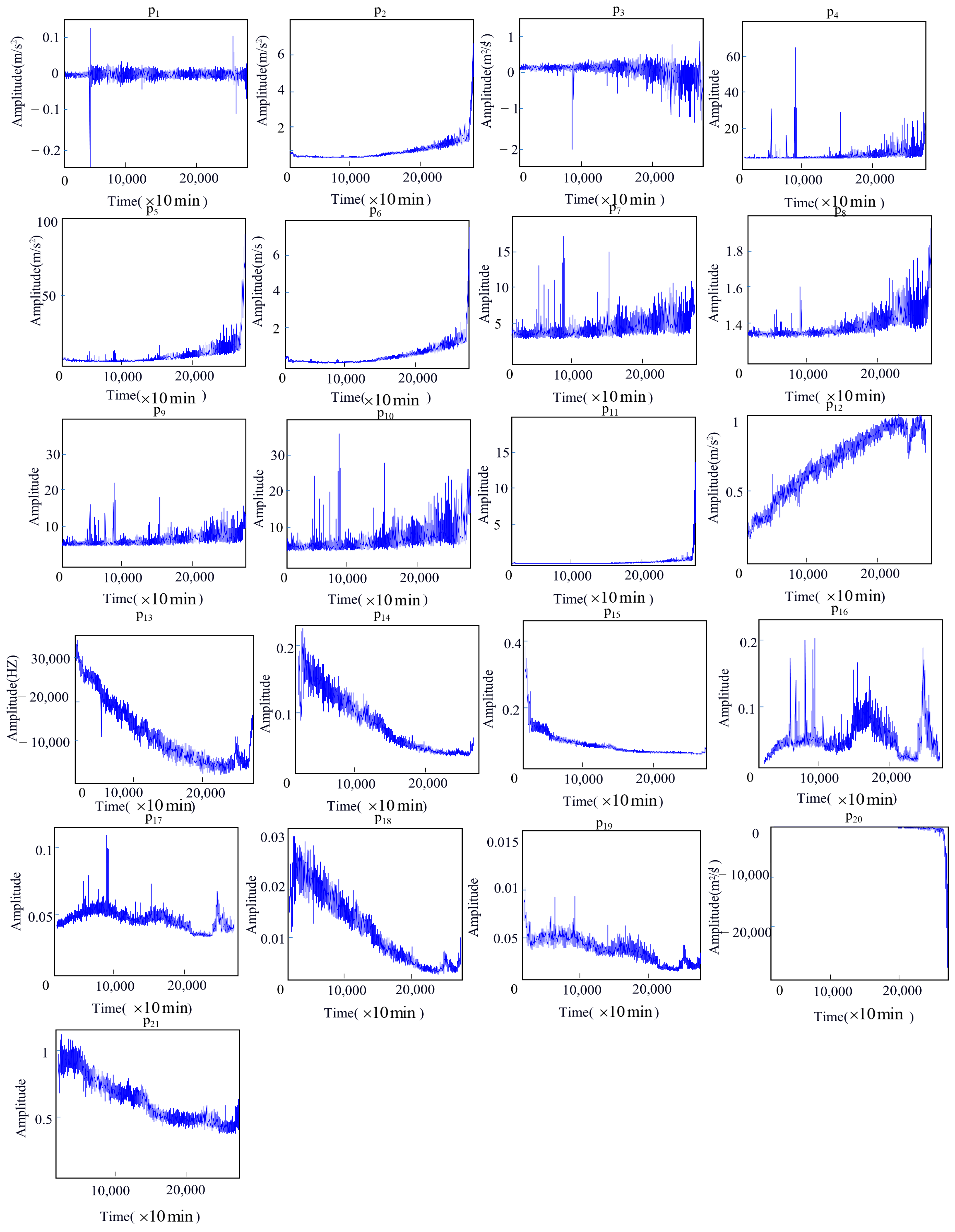
2.2.1. Multi-Domain Feature Extraction

Time, frequency, and time-frequency domain features are extracted [35], as shown in

Table 1. Feature expressions.

Serial Number	Name	Feature Expression
1	Mean	$p_1={\displaystyle \frac{{\displaystyle \sum _{i=1}^N{x}_i}}{N}}$
2	Standard Deviation	$p_2=\sqrt{{\displaystyle \frac{{\displaystyle \sum _{i=1}^N{(x_i-p_1)}^2}}{N}}}$
3	Variance	$p_3={\displaystyle \frac{{\displaystyle \sum _{i=1}^N{(x_i-p_1)}^2}}{N-1}}$
4	Skewness	$p_4={\displaystyle \frac{{\displaystyle \sum _{i=1}^N{x}_i^3}}{N}}$
5	Mean Square Root Value	$p_5=\sqrt{({\displaystyle \frac{{\displaystyle \sum _{i=1}^N{x}_i^2}}{N}}{)}^2}$
6	Root Mean Square Value	$p_6=\sqrt{{\displaystyle \frac{{\displaystyle \sum _{i=1}^N{x}_i^2}}{N}}}$
7	Kurtosis	$p_7={\displaystyle \frac{{\displaystyle \sum _{i=1}^N{x}_i^4}}{N}}$
8	Waveform	$p_8={\displaystyle \frac{p_5}{\left|p_1\right|}}$
9	Kurtosis	$p_9={\displaystyle \frac{p_7}{\left|p_6\right|}}$
10	Skewness	$p_{10}={\displaystyle \frac{N}{(N-1)(N-2)}}{\displaystyle \sum _{i=1}^N(\frac{x_i-p_1}{p_2}}{)}^3$
11	Peak	$p_{11}=\max (x(t_i))$
12	Mean Amplitude in Frequency Domain	$p_{12}={\displaystyle \frac{{\displaystyle \sum _{k=1}^N{s}_k}}{N}}$
13	Root Mean Square Frequency	$p_{13}={\displaystyle \frac{{\displaystyle \sum _{k=1}^N{(f_k)}^{2}s(k)}}{{\displaystyle \sum _{k=1}^{K}s(k)}}}$

Where x_i is the time domain signal sequence such that i = 1, 2, ⋯, N is the number of sample points, s(k) is the spectrum of signal x(n), k = 1, 2, ⋯, k is the number of spectral lines, and f_k is the frequency of the kth spectral line.

, where numbers 1–7 represent the time domain feature expressions, and numbers 8–13 represent the frequency domain feature expressions.

For the extraction of time-frequency domain features, the db6 function is used as the wavelet basis function, and the vibration signal is decomposed using three-layer wavelet packet decomposition to obtain 2³ = 8 seed frequency bands. The energy characteristics of these eight seed frequency bands are calculated to obtain the wavelet energy entropy [44]:

$$WEE=-{\displaystyle \sum _{i_o=1}^8(\frac{E_{i_o}}{E}\cdot \log (\frac{E_{i_o}}{E})})$$

(3)

where $E_{i_o}$ (where i_o denotes the i_o-th sub-frequency band) represents the energy characteristic of the i_o-th sub-frequency band, and E represents the total energy of all eight sub-frequency bands combined.

The energy ratio of each sub-frequency band is calculated using the following formula [44]:

$$P_{io}={\displaystyle \frac{E_{io}}{E}}\times 100\%$$

(4)

This allows us to estimate the energy ratios corresponding to different frequency sub-bands: p₁₄(3,0), p₁₅(3,1), p₁₆(3,2), p₁₇(3,3), p₁₈(3,4), p₁₉(3,5), p₂₀(3,6), and p₂₁(3,7) [44].

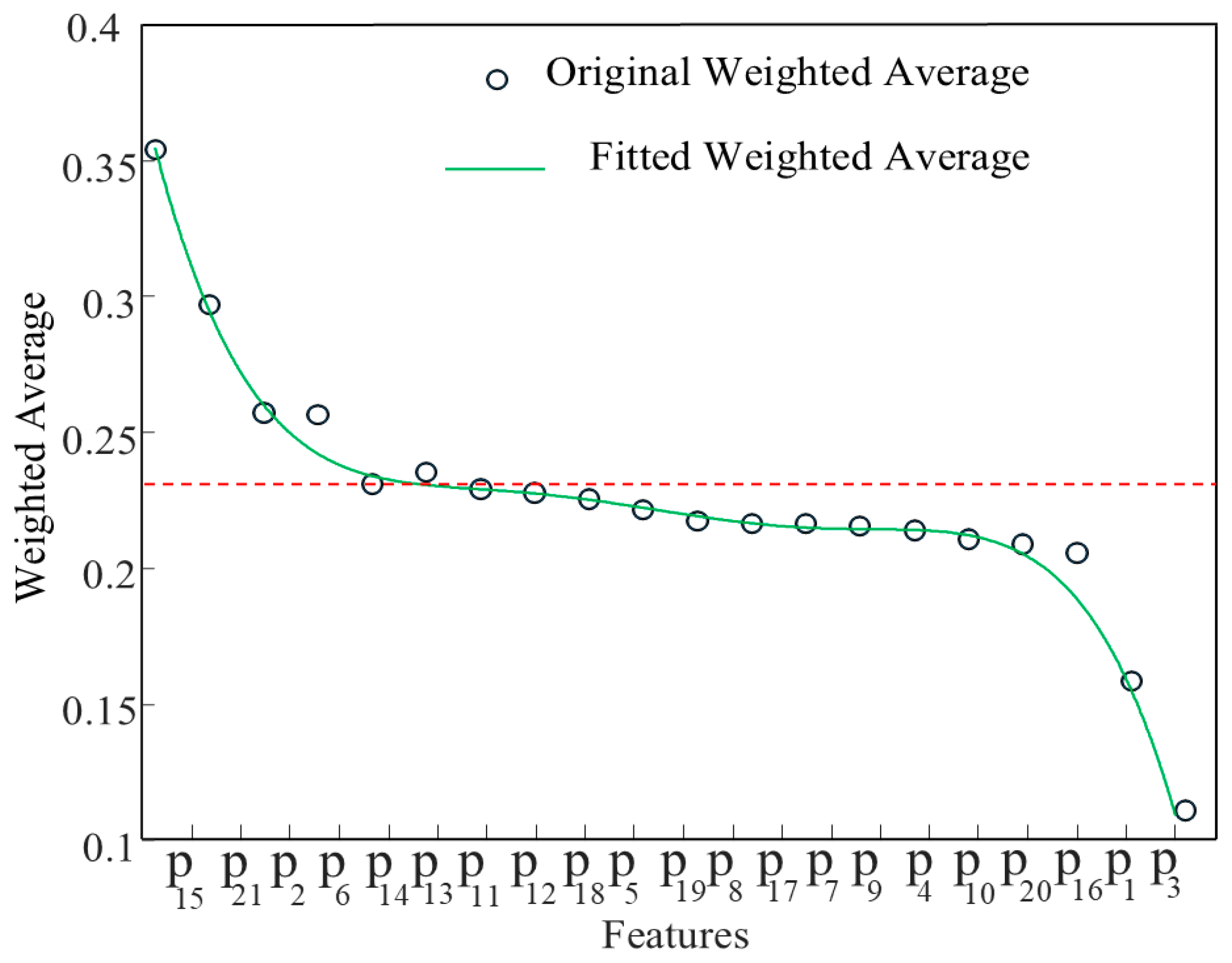
2.2.2. Sensitive Feature Selection

Different features have varying sensitivities to bearing degradation. In this paper, the monotonicity, trendability, predictability, and robustness [16] are used to comprehensively evaluate the sensitivity of the signal features. The weighted sum is calculated to determine a comprehensive score. Note that a higher score indicates higher sensitivity and greater contribution to the prediction of bearing life.

The Monotonicity indicator (M) determines the trend of a signal feature; it is expressed as [44]:

$$M={\displaystyle \frac{1}{m}}|{\displaystyle \frac{positivediff(x_{i_a}^n)-negativediff(x_{i_a}^n)}{k_a-1}}|$$

(5)

where x_i represents the i_a-th feature, k_a represents the number of measurements for each feature, and m is the number of monitored systems.

The Trendability indicator (Q) determines the correlation between the bearing running time and degradation features. It is computed as [44]:

$$Q={\displaystyle \frac{|{\displaystyle {\sum }_{i_b=1}^{No}(x_{i_b}-x_m)(y_{i_b}-y_m)}|}{\sqrt{{\displaystyle {\sum }_{i_b=1}^{No}{(x_{i_b}-x_m)}^2{\displaystyle {\sum }_{i_b=1}^{No}{(y_{i_b}-y_m)}^2}}}}}$$

(6)

where x_ib is the rank of features, y_ib is the rank of time, and N is the number of feature measurements. Note that, for Q = 1, the feature is strictly monotonic, while for Q = 0, it is non-monotonic.

The Predictability indicator (C) represents the ratio of the deviation (std) of the final failure value to the mean range of change for each feature. It is given by [44]:

$$C=\exp (-{\displaystyle \frac{std(f_{i_c}(N))}{mean|f_{i_c}(1)-f_{N_c}(N_c)|}})$$

(7)

where f_ic(1) and f_ic(N_c) are the initial and failure values of the i_c-th feature, respectively.

The Robustness indicator (R) represents the tolerance of specific features to existing outliers. Before calculation R, the underlying features should be smoothed using the local weighted scatter plot smoothing technique. It is expressed as [44]:

$$R=\frac{1}{N_R}{\displaystyle \sum _{i_R}\exp }(-{\displaystyle \frac{f_{i_R}-\tilde{f}}{f_{i_R}}})$$

(8)

where $f_{i_R}$ is the i_R-th feature, N_R represents its measurement value, and $\tilde{f}$ is the average trend value.

The final score is calculated by the weighted sum of each indicator [44]:

$$Score{J}_{j_0}=w_1^{\prime }{M}_{j_0}+w_2^{\prime }{Q}_{j_0}+w_3^{\prime }{F}_{j_0}+w_4^{\prime }{R}_{j_0}$$

(9)

where $j_0$ represents the j₀-th indicator, $w_1^{\prime }$, $w_2^{\prime }$, $w_3^{\prime }$, $w_4^{\prime }$ represents the weight, and $w_1^{\prime }$ + $w_2^{\prime }$ + $w_3^{\prime }$ + $w_4^{\prime }$ = 1.

2.2.3. The Fusion of Sensitive Features

Using the Kernel Principal Component Analysis (KPCA) [35] method to reduce the dimensionality of the selected features, resulting in health indicators, the detailed steps are as follows [33]:

(1)

The sample matrix X, composed of feature vectors and b dimensions, is as follows [33]:

$$X_{cd}=\left[\begin{array}{cccc}{X}_{11}& X_{12}& \dots & X_{1b}\\ X_{21}& X_{22}& \dots & X_{2b}\\ \dots & \dots & \dots & \dots \\ X_{a1}& X_{a2}& \dots & X_{ab}\end{array}\right]$$

(10)

where $X_{cd}=\left\{X_{c1},X_{c2},\dots ,X_{cb}\right\}$ corresponds to the feature vector value of the vibration signal in the c-th row of the matrix.

(2)

Implement the mapping of X into the high–dimensional space $\Re$, samples in the input space are transformed via Φ, denoted as $X\to \Phi (X)$, and become sample points within the high-dimensional feature space $\Re$, where $\Phi (X)=\left[\Phi (x_1),\Phi (x_2),\cdots ,\Phi (x_b)\right]$, satisfying the centrality condition [33]:

$${\displaystyle \sum _{k=1}^n\Phi (x_k)}=0$$

(11)

The covariance matrix in $\Re$ is given by C [35]:

$$C={\displaystyle \frac{1}{b}}{\displaystyle \sum _{j=1}^b\Phi (x_j)}{[\Phi (x_j)]}^T$$

(12)

where $\Phi (x_j)$ represents the feature sample in $\Re$.

(3)

Calculate the eigenvalues and eigenvectors of the covariance matrix C. The eigenvectors thus obtained represent the principal component directions of the original sample space in the feature space $\Re$ [33]:

$$\lambda v=Cv$$

(13)

where $\lambda$ represents the eigenvalue of C, and v denotes the corresponding eigenvector in the feature space $\Re$.

(4)

Define the $M\times M$ matrix, $K_{cd}=K_{cd}(x_c,x_d)=\Phi (x_c)\Phi (x_d)$, the normalized feature vector is represented as v^g, (v^g, v^g) = 1, the expression for the f-th principal component S of the original sample is [33]:

$$S=(v^m,\Phi (x))={\displaystyle \sum _{c=1}^{M}K(x,x_c)}$$

(14)

(5)

Zero-mean processing is performed on matrix K [33]:

$$\stackrel{\_}{K}=K-P_{M}K-K{P}_M+P_{M}K{P}_M$$

(15)

where $P_M={\displaystyle \frac{1}{M}}I$, I is the identity matrix.

(6)

${\lambda }_k$ is an eigenvalue of matrix $\stackrel{\_}{K}$, the first l eigenvalues, whose contribution rates satisfy the following formula, are selected as principal components [33]:

$${\displaystyle \raisebox{1ex}{${\displaystyle \sum _{k=1}^l{\lambda }_k}$}\!\left/ \!\raisebox{-1ex}{${\displaystyle \sum _{d=1}^g{\lambda }_d}$}\right.}\ge 85\%$$

(16)

Based on the eigenvalues and eigen components obtained from the above formulas, the value obtained by fusing various features is used as an indicator of the bearing’s degradation trend.

3. Remaining Useful Life Prediction Algorithm Based on Double Bidirectional Long Short-Term Memory

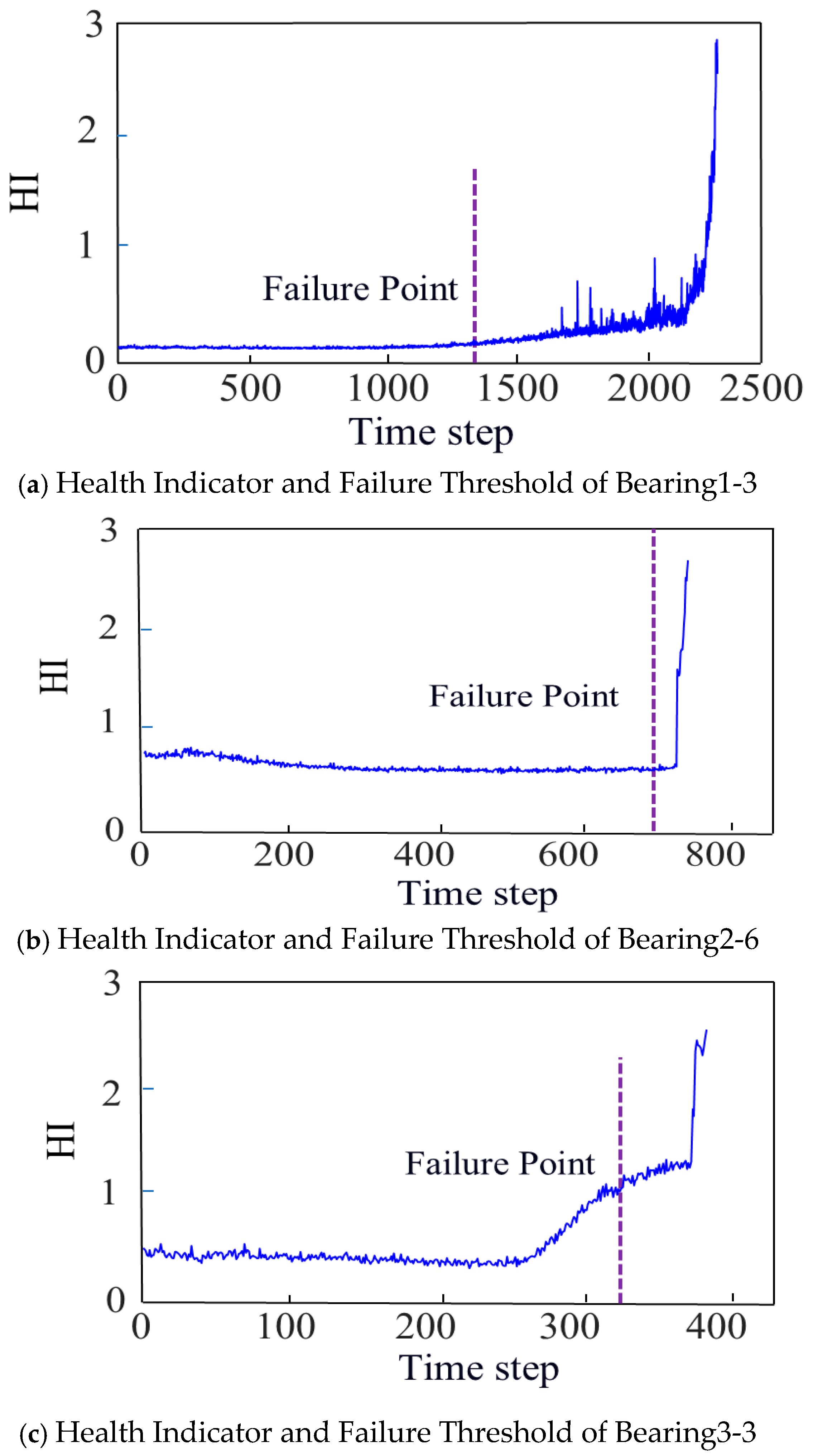
3.1. The Determination of Failure Thresholds

The failure threshold for bearings is established using the $3\sigma$ criterion, based on the description in the referenced literature [47,48,49,50,51,52,53]: approximately 99.73% of the data points will fall within the range defined by the mean (μ(t)) plus or minus three times the standard deviation (σ(t)), expressed as (μ(t) − 3σ(t),μ(t) + 3σ(t)); therefore, the 3σ criterion is widely applied in failure monitoring of bearings. The method and steps for determining the failure threshold of bearing signals are specifically as follows [48]:

(1)

The mean of the sample [48]:

$$\mu (t)={\displaystyle \sum _U^t{x}_i}$$

(17)

where U represents the length of the sample, and t represents the time point of the sample.

(2)

The standard deviation of the sample [48]:

$$\sigma (t)=\sqrt{{\displaystyle \frac{1}{U-1}}{\displaystyle \sum _U^t(x_i-\mu {(t)}^2)}}$$

(18)

(3)

The failure threshold of a bearing is represented by DT [48]:

$$|DT-\mu (t)|\ge 3\sigma (t)$$

(19)

(4)

Failure Judgment: An early warning mechanism will be triggered when condition $x(t)\ge \mu (t)+3\sigma (t)$ is met.

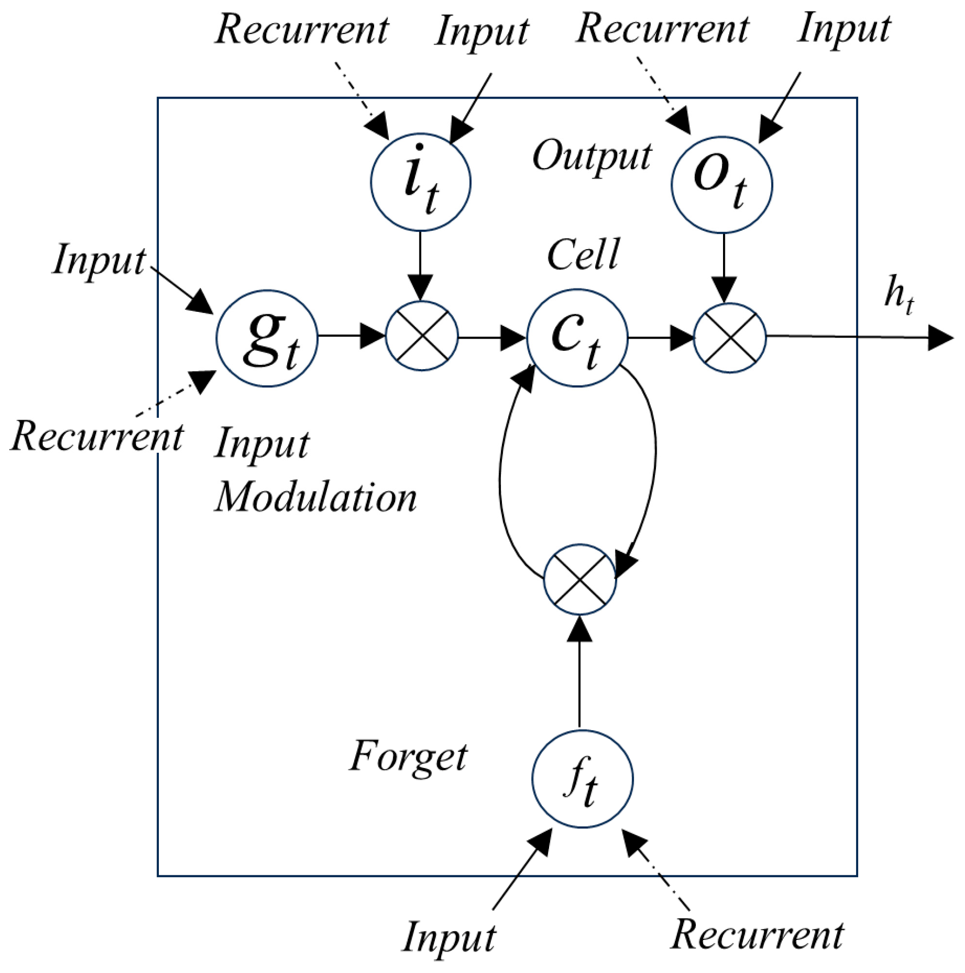
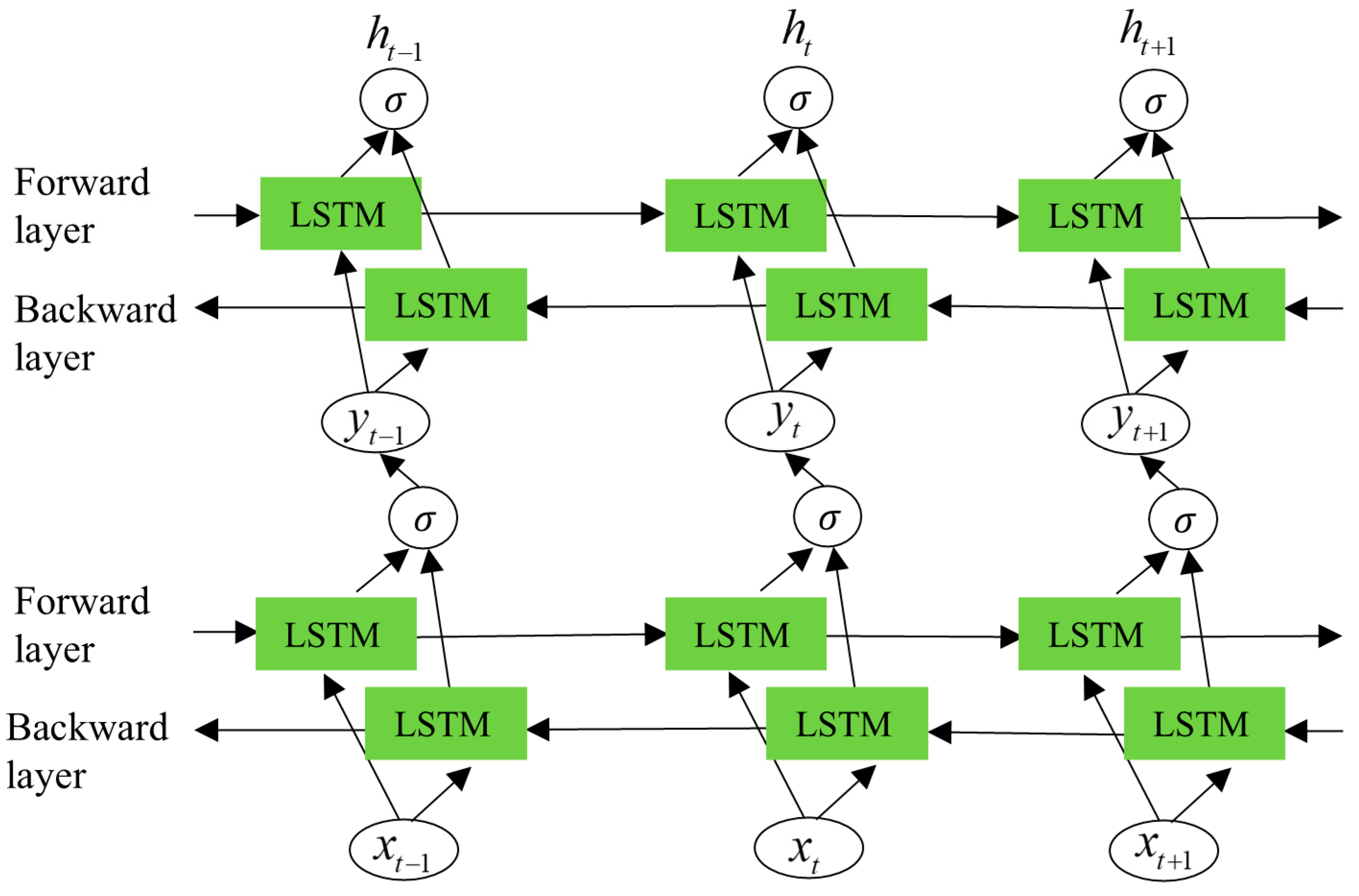
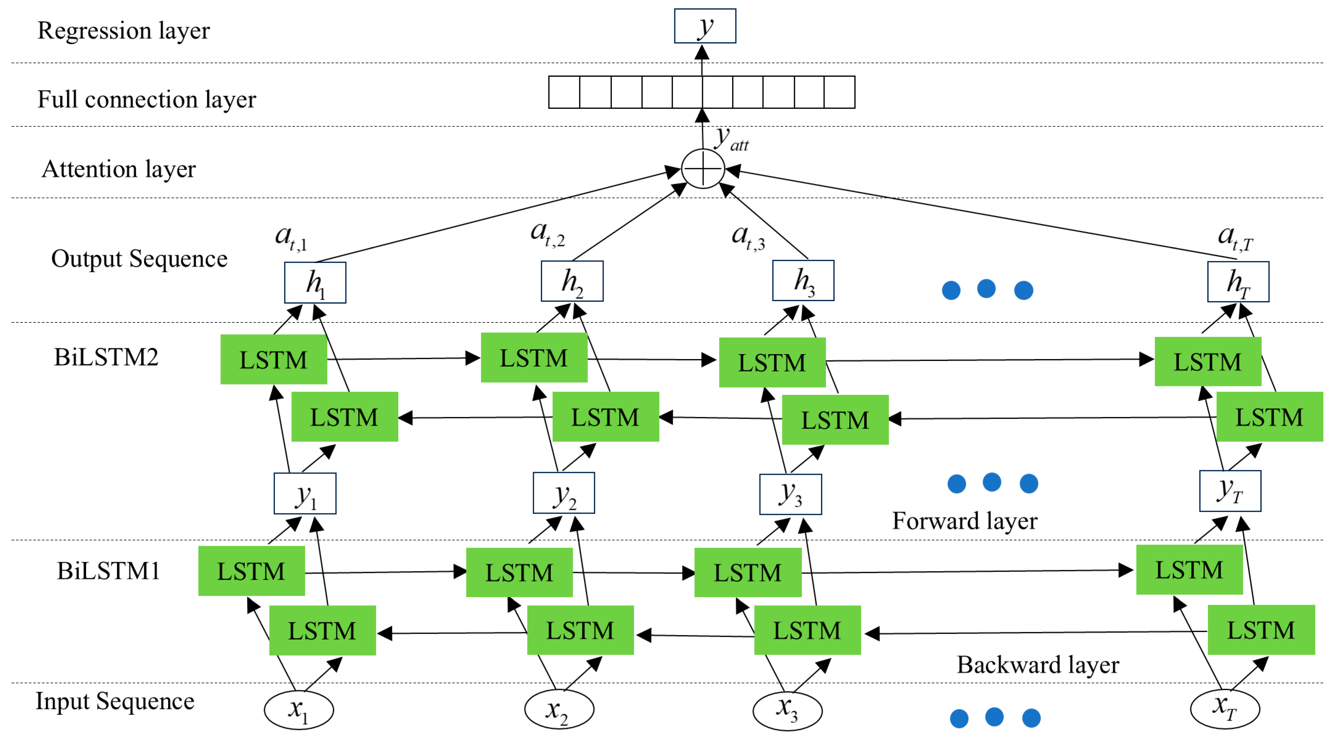
3.2. Principle of Double Bidirectional Long Short-Term Memory (DBiLSTM)

Memory cell of LSTM network [37] is shown in Figure 3; the memory cells of the LSTM form a hidden layer composed of different nodes: input, output, and forget gates [38,39,40]. The selective operations of these gates allow us to save specific information, and thus the LSTM networks can avoid gradient vanishing. During backpropagation, the weights of the memory units are adjusted, which allows the LSTM to retain the underlying information. The LSTM has high performance when dealing with long-term dependencies between input and output.

After network iteration activation, input sequence X = [x₁, x₂, …, x_n] is mapped to output h = [h₁, h₂, …, h_n]. At time step t = [1, 2, …, t − 1, …, T], the corresponding gates in LSTM units are expressed as [40]:

$$i_t=\sigma ({\omega }_{ix}{x}_t+{\omega }_{ih}{h}_{t-1}+b_i)$$

(20)

$$f_t=\sigma ({\omega }_{fx}{x}_t+{\omega }_{fh}{h}_{t-1}+b_f)$$

(21)

$$g_t=\tanh ({\omega }_{gx}{x}_t+{\omega }_{gh}{h}_{t-1}+b_g)$$

(22)

$$o_t=\sigma ({\omega }_{ox}{x}_t+{\omega }_{oh}{h}_{t-1}+b_o)$$

(23)

$$c_t=\sigma (g_t\otimes i_t+{\omega }_{ih}\otimes c_{t-1})$$

(24)

$$h_t=\phi (c_t)\otimes o_t$$

(25)

where, ${\omega }_{ix}$, ${\omega }_{fx}$, ${\omega }_{gx}$, and ${\omega }_{ox}$ represent the weight matrices between the input layer and corresponding gates at time t, ${\omega }_{ih}$, ${\omega }_{fh}$, ${\omega }_{gh}$, and ${\omega }_{oh}$ represent the weight matrices of the hidden layer between time values t and t − 1, $b_i$, $b_f$, $b_g$, and $b_o$, respectively, represent the bias values of the input, forget, control, and output gates, $h_{t-1}$ and $c_{t-1}$, respectively, represent the hidden and cell states of the previous time value t − 1, $i_t$, $f_t$, $g_t$, and $o_t$, respectively, represent the output values of the input, forget, control, and output gates, $c_t$ and $h_t$, respectively, represent the current cell state and hidden state at time t, $\phi$ and $\sigma$, respectively, represent the tanh and sigmoid activation functions, and $\otimes$ represents the point-wise multiplication operator.

BiLSTM can capture information from previous and following events. It combines two LSTM hidden layers to increase the performance of individual LSTM units. The input sequence X = [x₁, x₂, …, x_n] is processed by BiLSTM, generating hidden sequences in forward and backward directions. The forward and backward hidden sequences are, respectively, denoted by $\overrightarrow{h}=[\overrightarrow{h},\overrightarrow{h},\dots ,\overrightarrow{h}]$ and $\overleftarrow{h}=[\overleftarrow{h},\overleftarrow{h},\dots ,\overleftarrow{h}]$, and the concatenation of forward and backward outputs is considered as the final output. The encoding vector produced by the two hidden layers is expressed as [40]:

$$y_t=\sigma ({\omega }_{y\overrightarrow{h}}{\overrightarrow{h}}_t+{\omega }_{y\overleftarrow{h}}{\overleftarrow{h}}_t+b_y)$$

(26)

$${\overrightarrow{h}}_t=\sigma ({\omega }_{\overrightarrow{h}x}{x}_t+{\omega }_{\overrightarrow{h}\overrightarrow{h}}{\overrightarrow{h}}_{t-1}+b_{\overrightarrow{h}})$$

(27)

$${\overleftarrow{h}}_t=\sigma ({\omega }_{\overleftarrow{h}x}{x}_t+{\omega }_{\overleftarrow{h}\overleftarrow{h}}{h}_{t+1}+b_{\overleftarrow{h}})$$

(28)

$$h_t={\omega }_{\overrightarrow{h}\overrightarrow{h}}{\overrightarrow{h}}_t+{\omega }_{\overleftarrow{h}\overleftarrow{h}}{\overleftarrow{h}}_t+b_h$$

(29)

where $y_t=[\overrightarrow{h},\overleftarrow{h}]$ is the network output represented in the first hidden layer by y_t = [y₁, y₂, …, y_t, …, y_n]. In Double BiLSTM, the output of the previous layer is the input of the following layer, as shown in Figure 4.

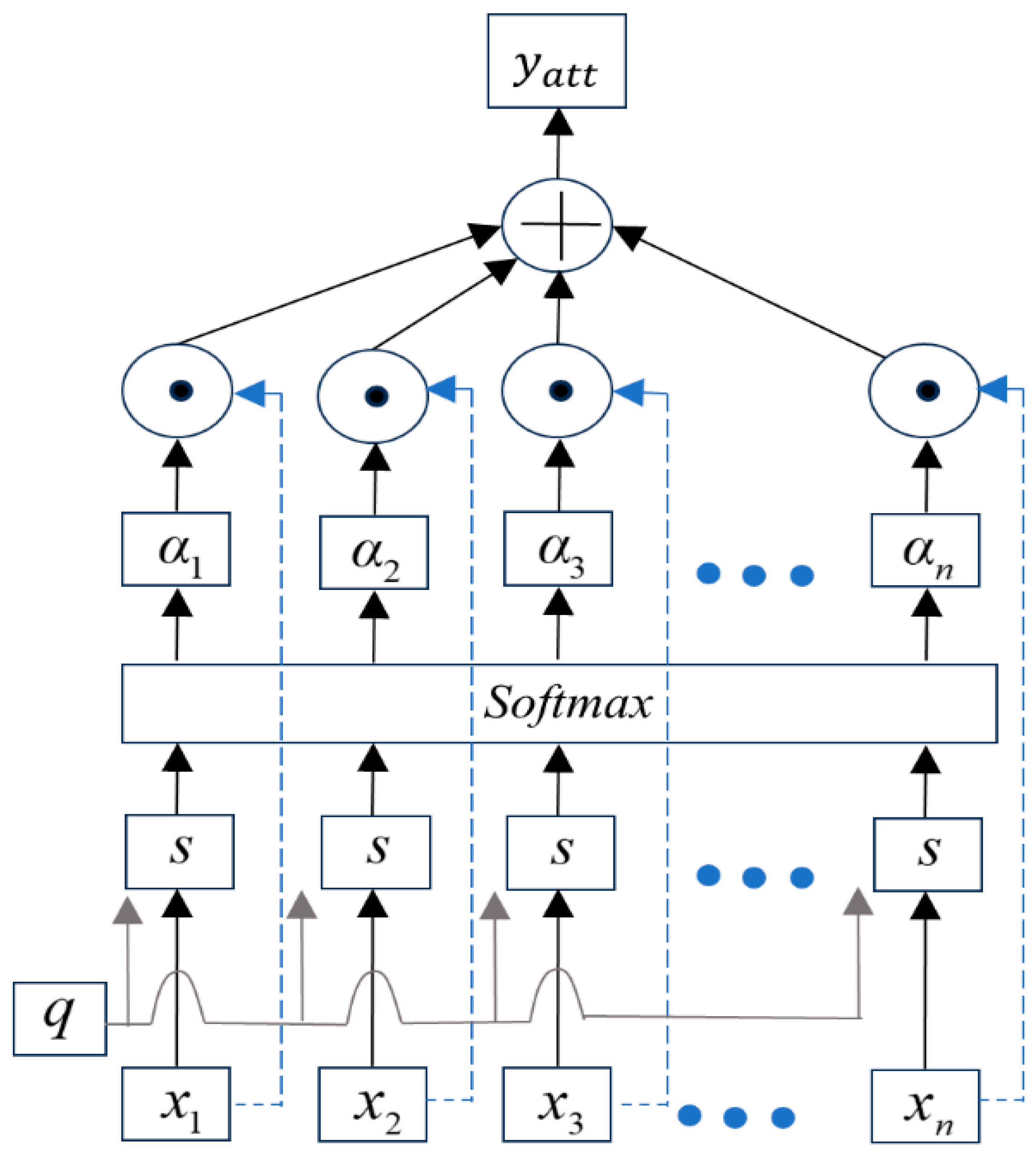
3.3. The Principle of Attention Mechanism Network

The attention mechanism assists the training of data performed by the BiLSTM model. More precisely, it helps the model focus on key information in sequences and increases its sensitivity to important time points. It selects task-relevant information from input sequences and allocates corresponding weights [1,2,3].

The input information is denoted by X = [x₁, x₂, …, x_n], where n is the number of inputs. For a given query q, the attention variable m ∈ R_n is used to index selected information from input sequence x. The probability of selecting the ith information, denoted by ${\alpha }_i$, is expressed as [15]:

$${\alpha }_i=p(m=i | n,q)={\displaystyle \frac{\exp (s(x_i,q))}{{\displaystyle {\sum }_{j=1}^n\exp (s(x_i,q))}}}$$

(30)

where $s(x_i,q)$ represents the scoring function, and ${\alpha }_i$ represents the attention coefficient.

$s(x_i,q)$ is given by [15]:

$$s(x_i,q)=q^T{x}_i$$

(31)

The output of the attention layer is obtained by first calculating attention weights for each input vector, then implementing a soft attention mechanism [16] to summarize input information in order to evaluate the bearing degradation function of time. Figure 5 shows the network structure.

$$y_{att}={\displaystyle \sum _{i=1}^n{\alpha }_n{x}_n}$$

(32)

The attention mechanism of the DBiLSTM output layer H is given by [44]:

$$\alpha =Soft\max (s(H,q))$$

(33)

$$y_{att}=\tanh (H{\alpha }^T)$$

(34)

The final output y_att represents high-level abstract information of the input, which is used to evaluate the bearing degradation function of time.

3.4. RUL Prediction Model

3.4.1. RUL Prediction Network Model Process

The RUL prediction mainly involves two steps: training and testing. Training set ${\left\{X_t,Y_t\right\}}_{t=1}^T$ (where $X_t\in {\Re }^{N_1\times 1}$ contains N₁ features at time t and Y_t is the true label related to bearing degradation at time t) is considered as the network input. Through Double BiLSTM layers, a deep structure is designed to simultaneously process past and future temporal information. In addition, the bearing degradation information propagates in forward and backward directions through the Double BiLSTM layers.

The network structure is shown in Figure 6. It combines DBiLSTM with attention mechanism. Two BiLSTM layers are double: BiLSTM1 and BiLSTM2. The former serves as input to the latter BiLSTM2. The final hidden state is multiplied by attention weights (a_t,1, a_t,2, a_t,3, …, a_t,T), and the results are added to generate the final output of the network (y_att). Attention weights are assigned to input data vectors, selecting highly relevant information from long-distance input sequences. RUL values are obtained through the regression layer. The model in the regression layer [37]:

$$L={{\displaystyle \frac{1}{T}}{\displaystyle \sum _{t=1}^T\Vert Y_t-{\widehat{Y}}_t\Vert }}_2^2$$

(35)

where Y_t is the true label of input data, ${\widehat{Y}}_t$ is the value predicted by the DBiLSTM network, and T denotes the total time points of the samples. During the testing phase, selected prognostic-sensitive features are directly input into the trained DBiLSTM network, which yields RUL values.

3.4.2. Bayesian Optimization for Hyperparameters

We automatically search for hyperparameters of the proposed remaining useful life prediction model and use the Bayesian optimization method [45] to achieve automatic optimization, thereby avoiding the cumbersome process of manually tuning hyperparameters.

The objective function of Bayesian optimization is the prediction error on the validation set. In this paper, RMSE (Root Mean Squared Error) is adopted; the formula for RMSE is [5]:

$$RMSE=\sqrt{{\displaystyle \frac{1}{n_y}}{\displaystyle \sum _{i=1}^{n_y}{(Y_t-{\hat{Y}}_t)}^2}}$$

(36)

where $n_y$ represents the number of samples in the test set.

Formulas related to Bayesian optimization are obtained from Reference [45]:

(1)

The objective search formula is designed as:

$$f(\theta )=Error(Y_t,{\hat{Y}}_t)$$

(37)

where θ represents the combination of hyperparameters (learning rate, number of hidden layer neurons, batch size, dropout rate, and number of iterations).

(2)

Bayesian optimization models the objective function through a Gaussian process, with the assumption that:

$$f(\theta )\sim GP(m(\theta ),k_h(\theta ,{\theta }^{\prime }))$$

(38)

where m(θ) is the mean function (usually set to 0), and k_h(θ,θ′) is the kernel function, whose formula is:

$$k_h(\theta ,{\theta }^{\prime })={\sigma }_f^2\exp (-{\displaystyle \frac{{‖\theta -{\theta }^{\prime }‖}^2}{2l_l^2}})$$

(39)

(3)

Given the observed data $D={\left\{({\theta }_{ii},f({\theta }_{ii}))\right\}}_{ii=1}^{n_y}$ (where $n_y$ represents the number of samples in the test set, and ii = 1,2, …, $n_y$), the posterior distribution remains a Gaussian process, with its mean and variance given by:

$$\mu (\theta )=K_0^T{(K_{00}+{\sigma }_{n_y}^{2}I)}^{-1}f$$

(40)

$${\sigma }^2(\theta )=k_h(\theta ,\theta )-K_0^T{(K_{00}+{\sigma }_{n_y}^{2}I)}^{-1}{K}_0$$

(41)

where $K_0$ is the vector of kernel function values between the new point θ and the observed points θ_ii, $K_{00}$ is the kernel function matrix among the observed points, and ${\sigma }_{n_y}^2$ is the variance of the observation noise.

(4)

An acquisition function is used to select the next evaluation point. The main formula is:

Expected Improvement:

$$a_{EI}(\theta )=E[\max (0,f_{best}-f(\theta ))]$$

(42)

where f_best is the current optimal value.

Upper Confidence Bound:

$$a_{UCB}(\theta )=\mu (\theta )+\kappa \sigma (\theta )$$

(43)

where κ controls the balance between exploration and exploitation and is the uncertainty coefficient.

The search ranges when optimizing hyperparameters using Bayesian optimization are as follows: number of neurons in hidden layers: [16, 512]; initial learning rate: [10⁻⁴, 1]; batch size: [16, 512]; number of iterations: [50, 3000]; dropout rate: [0, 0.5].

4. Experimental Validation and Result Analysis

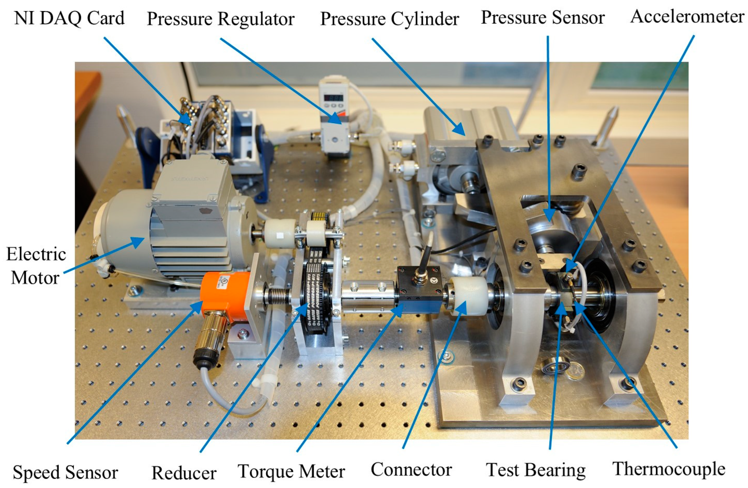
4.1. Processing of Experimental Data

The superiority of the proposed method is demonstrated on the IEEE PHM2012 dataset. The experimental platform is shown in Figure 7. A sampling frequency of 25.6 KHz is adopted; that is, 2560 samples are collected every 10 s. The dataset can be found in the literature [54]; in this paper, the training and test sets are shown in

Table 2. Bearing dataset.

Conditions	Training Set	Testing Set
Condition 1	Bearing 1-1~Bearing 1-2	Bearing 1-3
Condition 2	Bearing 2-1~Bearing 2-2	Bearing 2-6
Condition 3	Bearing 3-1~Bearing 3-2	Bearing 3-5

. Horizontal vibration signals contain more degradation information, and therefore they are used in the conducted experiments.

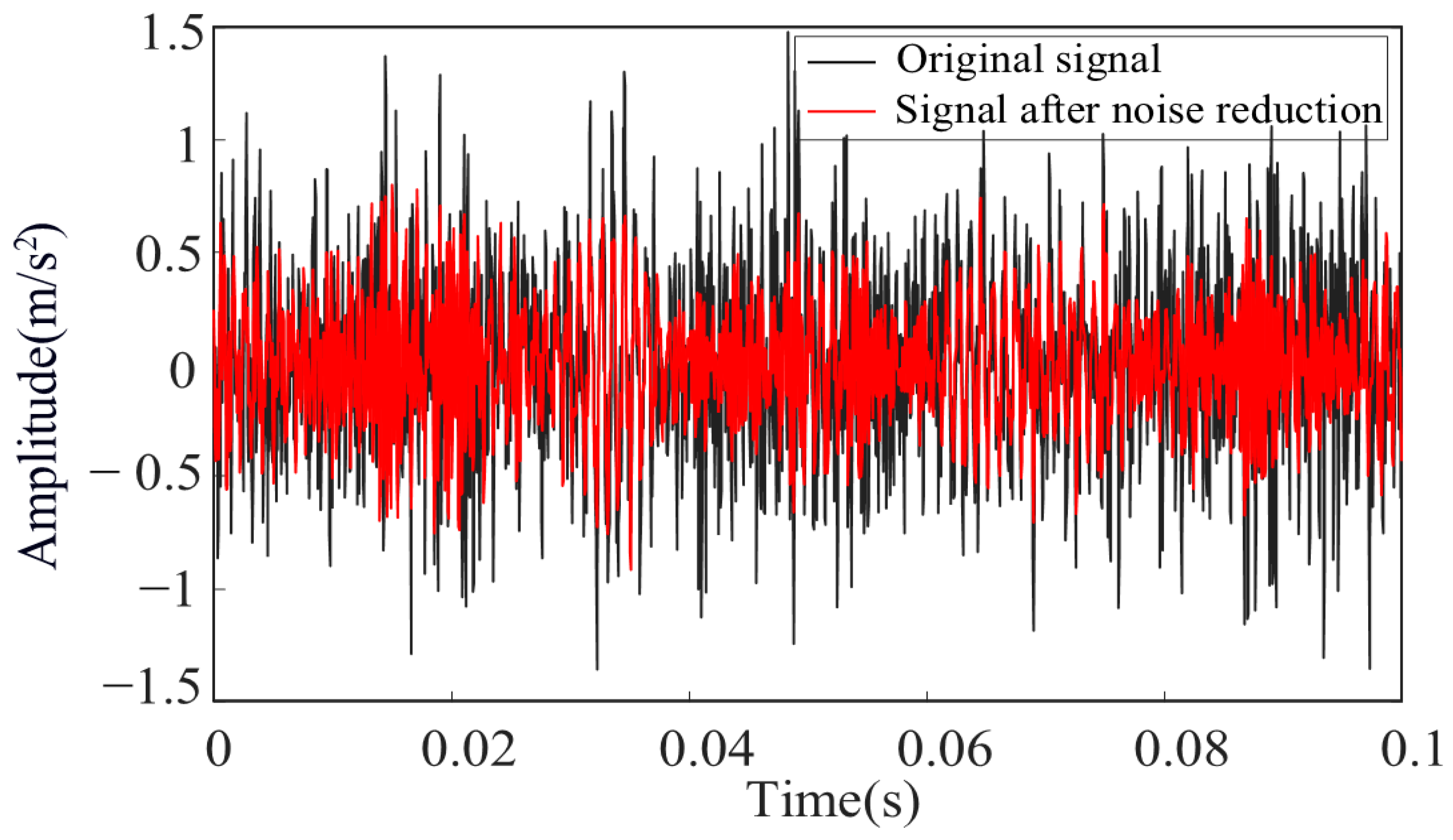
4.1.1. Result of Experimental Data Denoising

According to the data signal processing method described in Section 2.1, the dataset Bearing1-3 is as an example, and denoising processing is applied to the bearing dataset. As shown in Figure 8, it presents a comparison of the vibration signals before and after denoising. As shown in

Table 3. The result of signal denoising.

Evaluation Method	PSO-VMD	Wavelet Soft Thresholding
RMSE	0.0153	0.032
RMS	0.123	0.179
MAE	0.00008	0.000012

, we use RMSE (Root Mean Squared Error), RMS (Root Mean Square), and MAE (Mean Absolute Error) to evaluate the denoising performance, and compared with the classical Particle Swarm Optimization-based Variational Mode Decomposition denoising algorithm (PSO-VMD).

The formula for RMSE is [5]:

$$RMSE=\sqrt{{\displaystyle \frac{1}{n_o}}{\displaystyle \sum _{o=1}^{n_o}{(z_o-{\hat{z}}_o)}^2}}$$

(44)

where $z_o$ represents the original vibration signal, ${\hat{z}}_o$ denotes the signal after denoising treatment, and n is the number of samples.

The formula for RMS is [8]:

$$RMS=\sqrt{{\displaystyle \frac{1}{n_o}}{\displaystyle \sum _{o=1}^{n_o}{{\hat{z}}_o}^2}}$$

(45)

The formula for MAE is [8]:

$$MAE={\displaystyle \frac{1}{n_o}}{\displaystyle \sum _{o=1}^{n_o}\left|z_o-{\hat{z}}_o\right|}$$

(46)

It can be seen that the RMSE, RMS, and MAE values obtained using the wavelet threshold denoising algorithm are 0.032, 0.079, and 0.000012, respectively, which are all smaller than those of the comparative algorithm PSO-VMD. Therefore, the wavelet threshold algorithm exhibits stronger denoising capability. Through denoising processing, the bearing signal becomes purer, with improved signal quality, thus providing an accurate data foundation for subsequent feature extraction, failure threshold detection, and life prediction of bearing signals.

4.1.2. Sensitive Feature Selection Results

Considering Bearing1-3 as an example, features are then extracted using the method presented in Section 2.2. Seven time-domain, six frequency-domain, and eight time-frequency domain features are finally extracted; the 21 features are illustrated in Figure 9. These features each have their own advantages. For example, the time-domain features of P₁–P₆ are characterized by changes in signal waveform over time. The frequency-domain features of P₇–P₁₄ represent the distribution of different signal characteristics in the frequency spectrum, allowing for the study of signal curve characteristics from the spectrum. The time-frequency domain features of P₁₅–P₂₁ can capture the instantaneous characteristics of signals, reflecting fault information of bearing vibration signals from different perspectives. According to reference [44], the performance of bearings changes over time. When predicting bearing life, the focus is primarily on long-term trends. Predictability represents the accuracy of the model, and a model with strong robustness can provide more stable predictions of bearing life. The weights for each indicator are 0.5, 0.35, 0.05, and 0.1, respectively. The weight scores for each feature are shown in

Table 4. The weighted averages.

Feature	Monotonieity	Trendability	Prognosability	Robustness	J
p1	0.020	0.003	0.323	0.417	0.07
p2	0.075	0.324	0.454	0.955	0.27
p3	0.018	0.008	0.240	0.462	0.07
p4	0.020	0.022	0.567	0.831	0.13
p5	0.034	0.230	0.460	0.858	0.21
p6	0.075	0.318	0.454	0.955	0.27
p7	0.019	0.013	0.656	0.864	0.13
p8	0.021	0.028	0.621	0.983	0.15
p9	0.015	0.012	0.644	0.853	0.13
p10	0.017	0.007	0.642	0.850	0.13
p11	0.063	0.241	0.247	0.913	0.22
p12	0.175	0.018	0.499	0.916	0.21
p13	0.162	0.463	0.553	0.915	0.36
p14	0.211	0.091	0.400	0.896	0.25
p15	0.162	0.576	0.925	0.905	0.42
p16	0.166	0.033	0.525	0.896	0.21
p17	0.047	0.025	0.553	0.894	0.15
p18	0.170	0.040	0.400	0.887	0.21
p19	0.109	0.027	0.522	0.886	0.18
p20	0.023	0.043	0.151	0.886	0.12
p21	0.174	0.116	0.254	0.967	0.24

.

The fitted data of weighted averages for each indicator are arranged in descending order, as shown in Figure 10. It can be seen that when the weighted average is almost 0.23 (as indicated by the position of the red dashed line in Figure 10), the curve shows a significant turning trend. This is consistent with the result obtained in [16]. For sensitive feature selection, features with weighted averages ($J$) greater than 0.23 are selected.

The selected features are p₂, p₆, p₁₃, p₁₄, p₁₅, and p₂₁, as shown in Figure 11. These features demonstrate either monotonic increase or decrease. This indicates that, when the degradation increases, the vibration signal amplitude also increases with monotonically increasing features, while monotonically decreasing features describe the reduction in bearing RUL function of time. These features encompass most of the degradation information of bearings, and these sensitive prognostic features significantly contribute to mapping accurate bearing health conditions, providing a reference for precise RUL prediction.

4.1.3. Feature Fusion and Failure Threshold

As shown in

Table 5. Detection of failure points by the 3σ and actual failure points.

Bearings	3σ (Failure Points (min))	RMS (Failure Points (min))	Actual Operating (min)
1-3	1330	1414	2311
2-6	673	688	701
3-3	323	328	434

, the Bearing failure times detected using the 3σ threshold setting method and the RMS threshold setting method [8], respectively, are compared with the actual operational times. It can be observed from Table 5 that the failure points (The unit is “min”) detected by the 3σ method for the three bearing datasets are 1330, 673, and 323, respectively, the RMS method for the three bearing datasets are 1414, 688, and 328, respectively, while the actual operating times of the bearings are 2311, 701, and 434. The detected failure times are earlier than the actual operating times of the bearings; however, the 3σ method detects bearing failure earlier than the RMS method. This detection method can identify the degradation state of the bearings in advance, avoid missed detections, and guide staff to prepare preventive measures in advance.

Figure 12 shows the HI curves and failure thresholds for the three types of data, the unit of the time step is minute. It can be observed that, although the operating conditions in Figure 12a,b are the same, their HI curves and failure thresholds are different. This is due to the fact that, despite using the same model of bearings for the same operating conditions, the manufacturing and processing of individual bearings are different, which leads to different results. The operating condition presented in Figure 12c is different from those presented in Figure 12a,b. This results in different operating times, HI curves, and failure thresholds.

4.2. RUL Prediction Process and Result Analysis

4.2.1. RUL Prediction Process

The operating system of the computer used is Windows 11, 64-bit, with a processor of Intel(R) Core (TM) i7-10875H/NVIDIA GeForce RTX 2060, and the deep learning framework is MATLAB v2024a. To ensure fair comparison with other neural network models, the deep learning networks used for comparison are BiGRU (Bidirectional Gated Neural Network) and CNN-LSTM (Hybrid Model of Convolutional Neural Network and LSTM Network).

The size of the hidden units significantly affects the network prediction performance. Insufficient hidden units lead to poor feature learning, while a large number increases the complexity of the network. Therefore, in this paper, the BiLSTM layer hidden units are determined through minimum validation loss. The selection of hidden units is performed by calculating the validation loss of each pair of hidden units (H1, H2), which correspond to the first and second BiLSTM layers, respectively. The forward and backward layers of each BiLSTM have the same number of hidden units, while the output layer size is equal to 1. The A-DBiLSTM model output is flattened through fully connected layers and maintained in the range of 0–1 using a sigmoid activation function. Regression is performed on the final output to predict RUL labels, and the RMSE is used as the loss function of the regression layer, the network hyperparameters obtained through Bayesian automatic optimization. In this study, the RUL prediction process aims at optimizing the training of the network by learning current health conditions from short sequence data.

The parameter settings of the RUL prediction model mentioned in

Table 6. Detailed network structure.

Model	Layer Name	Detailed Description
Prosed method	BiLSTM1, BiLSTM2, Fully connected layer, Regression layer	Number of hidden layer neurons: BiLSTM1 = 93, BiLSTM2 = 93; Fully connected layer: layer1 = 40, layer2 = 25, Output vector dimension:1; Learning rate: 0.0098; Batch size: 64; Number of iterations: 2000; Dropout rate: 0.147; Activation function: Relu. Regression layer = 1
BiGRU	GRU, Fully connected layer, Regression layer	Number of hidden layer neurons: 240; Fully connected layer: 40; Output vector dimension: 1; Learning rate: 0.001; Batch size: 64; Number of iterations: 2000; Dropout rate: 0.15; Activation function: Relu. Regression layer = 1
CNN-LSTM	1DConv1, 1DConv1, LSTM, Fully connected layer, Regression layer	Number of hidden layer neurons: 128; Fully connected layer: layer1 = 40, layer2 = 25; Output vector dimension: 1; Pooling = {1*2}, Learning rate: 0.001; Batch size: 64; Number of iterations: 2000; Dropout rate: 0.015; Activation function: Relu. Regression layer = 1

. Additionally, it lists the network parameters of the comparative algorithms BiGRU and CNN-LSTM.

The reliability of the prediction results of the proposed method is evaluated using a 95% confidence level, the formula for calculating the confidence interval is as follows [49]:

$$CON=[{\hat{\mu }}_{con}-z_{\delta /2}\cdot {\displaystyle \frac{s}{\sqrt{n_y}}},{\hat{\mu }}_{con}+z_{\delta /2}\cdot {\displaystyle \frac{s}{\sqrt{n_y}}}]$$

(47)

where ${\hat{\mu }}_{con}$ represents the sample mean of multiple prediction results. In the paper, predictions are repeated 50 times. $z_{\delta /2}$ denotes the quantile of the standard normal distribution, with a confidence level of 95%, $z_{\delta /2}$ = 1.96, s stands for the standard deviation of the prediction results, and $n_y$ represents the sample size of the test set [49].

Calculate the average of all prediction results [49]:

$${\hat{\mu }}_{con}={\displaystyle \frac{1}{n_y}}{\displaystyle \sum _r^{n_y}{x}_r}$$

(48)

where $x_r$ denotes the prediction result for the r-th time.

Calculate the standard deviation of the prediction results [49]:

$$s={\displaystyle \frac{1}{n_y-1}}\sqrt{{\displaystyle \sum _r^{n_y}(x_r}-{\hat{\mu }}_{con}{)}^2}$$

(49)

The level of significant difference between the proposed RUL prediction model and the comparative models can be described as follows [55]: Null hypothesis (H₀): there is no significant difference between the predicted results of the proposed model and the comparison model; alternative hypothesis (H₁): there is a significant difference between the proposed model and the comparison model.

Mean difference [55]:

$$\stackrel{-}{d}={\displaystyle \frac{1}{n_y}}{\displaystyle \sum _{r-1}^{n_y}{d}_r}$$

(50)

where $d_r$ denotes the difference between the proposed model and the comparison model, and $d_r={\hat{Y}}_t-Y_c$, $Y_c$ is the RUL of comparison model.

Standard deviation of differences [55]:

$$s_d=\sqrt{{\displaystyle \frac{1}{n_y-1}}{\displaystyle \sum _r^{n_y}(d_r}-\stackrel{-}{d}{)}^2}$$

(51)

The test statistic is [55]:

$$t_d={\displaystyle \frac{\stackrel{-}{d}}{\frac{s_d}{n_y}}}$$

(52)

Degrees of freedom are denoted as $n_y-1$, by consulting the distribution table [55]: the significance level $\gamma$ = 0.05. If p < $\gamma$, reject the null hypothesis and consider that there is a significant difference between the proposed model and the comparative model.

The formula for calculating the p-value is as follows [55]:

$$p=\mathrm{t}.\mathrm{cdf}(t_d,\mathrm{df})$$

(53)

where df is the degrees of freedom, and t.cdf is the cumulative distribution function of the t-distribution.

To observe the performance of the proposed method more intuitively, Root Mean Squared Error (RMSE) and Absolute Error (MAE) are used as performance indicators to evaluate the effectiveness and superiority of the proposed method; the formula for RMSE has been defined in the previous Section 4.1.1, and the formula for MAE is as follows [8]:

$$MAE={\displaystyle \frac{1}{n_y}}{\displaystyle \sum _{i=1}^{n_y}|Y_t-{\hat{Y}}_t|}$$

(54)

The fitting performance of the model is evaluated using R²; the closer R² is to 1, the better the fitting degree of the model is proven to be [46]:

$$R^2=1-{\displaystyle \frac{{\displaystyle \sum _{i=1}^{n_y}{(Y_t-{\hat{Y}}_t)}^2}}{{\displaystyle \sum _{i=1}^{n_y}{(Y_t-\stackrel{-}{Y_t})}^2}}}$$

(55)

where $\stackrel{-}{Y_t}$ is the average value of the predicted RUL.

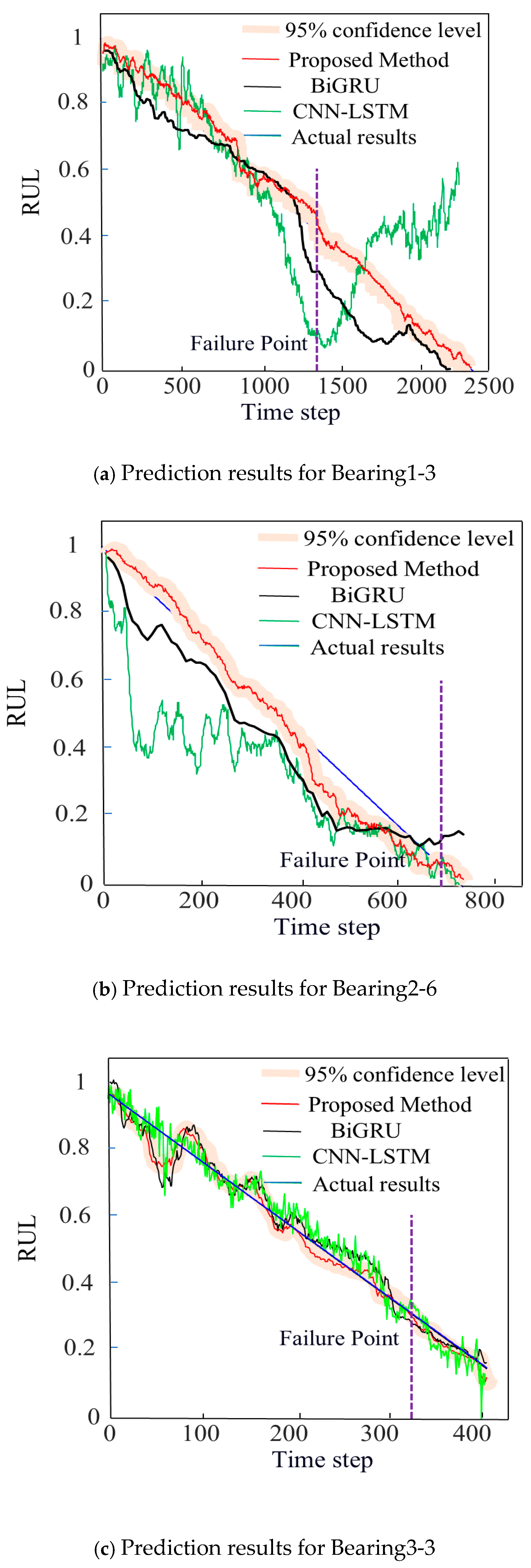
4.2.2. Prediction Result Analysis

Figure 13 shows the RUL prediction graphs for Bearing1-3, Bearing 2-6, the unit is minute, and Bearing 3-3; they belong to operating conditions 1, 2, and 3, respectively. It can be observed that the monotonically decreasing trend represents the bearing degradation time, the RUL predicted by the proposed method (A-DBiLSTM) is very close to the actual one; moreover, the RUL curve of the proposed method falls within the 95% confidence interval, and under different operating conditions, the predicted curves of the bearing’s RUL are all very close to the actual RUL curve.

It can also be seen from the figure that whether the BiGRU method or the CNN-LSTM method is used, there is a relatively large deviation between the predicted results and the actual results. In other words, their performance is lower than that of the proposed method. This indicates that the proposed method can provide sufficient preparation time for maintenance decisions, and reduces the economic losses caused by failure downtime.

As shown in

Table 7. Significance level of the RUL prediction results.

Bearings	The Proposed Method vs. BIGRU p-Value	The Proposed Method vs. CNN-LSTM. p-Value
1-3	p1-3 = 0.0188	p1-3 = 0.0001
2-6	p2-6 = 0.0012	p2-6 = 0.0082
3-3	p1-3 = 0.0234	p3-3 = 0.0329

, it presents the p-values when comparing the proposed RUL prediction method with the BiGRU prediction method and the CNN-LSTM prediction method. Based on Formulas (48) to (53), the p-values were calculated; upon analyzing the data in the table, it can be observed that in the datasets Bearing1-3, Bearing2-6, and Bearing3-3, the p-values between the proposed method and the BiGRU method are 0.0188, 0.0012, and 0.0234, respectively, and the p-values between the proposed method and CNN-LSTM are 0.0001, 0.0082, and 0.0329, respectively; all these values are less than the significance level $\gamma$ = 0.05, and p < 0.05; it indicates that there is a significant difference between the proposed model and the comparison model, leading to the rejection of the null hypothesis, and this indicates that the proposed method outperforms the comparison methods in terms of predictive performance, and the prediction results are reliable on all three datasets. This indicates that under different operating conditions, the proposed network model can reliably predict the RUL of bearings, demonstrating the applicability and generalizability of the proposed method.

As shown in

Table 8. Evaluation metrics of different methods.

Model	Bearings	RMSE	MAE	R2
	1_3	0.1033	0.0729	0.8920
Prosed method	2_6	0.1316	0.0975	0.9725
	3_3	0.0406	0.0296	0.9802
	1_3	0.0503	0.4354	0.8298
BiGRU	2_6	0.1368	0.1803	0.7753
	3_3	0.0532	0.0422	0.9660
	1_3	0.0503	0.1733	0.8821
CNN-LSTM	2_6	0.2216	0.1004	0.4372
	3_3	0.0554	0.0429	0.9632

, and the values of performance evaluation metrics MSE, MAE, and RMSE were obtained. By comparing the data in the table, it can be seen that the RMSE and MAE values of the proposed method are both smaller than those of the other two comparative methods; smaller MAE and RMSE values indicate better prediction performance of the RUL model. Moreover, the R² values of the proposed method are all greater than those of the other two comparative methods, and the closer the R² value is to 1, the higher the fitting degree of the network, indicating that the fitting degree of the proposed network model is superior to the other two. Combining this with Figure 13, it can be observed that compared with other methods, the RUL curve of the proposed prediction model has less overall fluctuation, which further proves that the proposed model is more in line with the actual situation.

4.2.3. Validation of the Generalization Ability of the Prediction Model

To further validate the generalization ability and adaptability of the proposed prediction mode, the XJTU-SY dataset from the literature [54] is employed for validation, with a sampling frequency of 25.6 kHz, a sampling interval of 1 min, and each sampling session lasting for 1.28 s. In this paper, the description of the dataset used for training and testing is as follows: Condition 1: radial force of 12,000 N at 2100 rpm, it includes the training set comprising Bearing1-1 to Bearing1-2, and the testing set is Bearing1-3; Condition 2: radial force of 11,000 N at 2250 rpm, it includes the training set comprising Bearing2-1 to Bearing2-2, and the testing set is Bearing2-5; Condition 3: radial force of 10,000 N at 2400 rpm, it includes the training set comprising Bearing3-1 to Bearing3-2, and the testing set is Bearing3-5.

Figure 14 illustrates the RUL prediction results for Bearing1-3, Bearing2-5, and Bearing3-5, the unit is minute, the failure points of the three datasets are 58 min, 120 min, and 6 min, respectively. As shown in

Table 9. Significance level of the RUL prediction results.

Bearings	The Proposed Method vs. BIGRU p-Value	The Proposed Method vs. CNN-LSTM. p-Value
1-3	p1-3 = 0.0196	p1-3 = 0.0001
2-6	p2-5 = 0.0012	p2-5 = 0.0083
3-3	p3-5 = 0.0241	p3-5 = 0.0327

, which presents the p-values when comparing the proposed RUL prediction method with the BiGRU prediction method and the CNN-LSTM prediction method, it also can be observed that in the datasets Bearing1-3, Bearing2-5, and Bearing3-5, the p-values between the proposed method and the BiGRU method are 0.0196, 0.0012, and 0.0241, respectively, and the p-values between the proposed method and CNN-LSTM are 0.0001, 0.0083, and 0.0327, respectively. All these values are less than 0.05; this result further demonstrates that when the proposed prediction model is applied to the XJTU-SY dataset, its prediction performance is equally satisfactory.

While

Table 10. Evaluation metrics of different methods.

Model	Bearings	RMSE	MAE	R2
	1_3	0.0682	0.0741	0.8743
Prosed method	2_5	0.0811	0.0591	0.9211
	3_5	0.0866	0.0533	0.9100
	1_3	0.0881	0.0567	0.8298
BiGRU	2_5	0.0917	0.0763	0.9090
	3_5	0.0899	0.0422	0.8570
	1_3	0.1255	0.0907	0.8538
CNN-LSTM	2_5	0.1666	0.0914	0.8863
	3_5	0.2166	0.4836	0.8782

shows the values of evaluation metrics including RMSE, MAE, and R². By combining the information from Figure 14 and Table 10, through comparative observation, it is found that when the proposed method is applied to the XJTU-SY dataset, both RMSE and MAE are smaller than those of the comparative methods, the prediction curve of the proposed method lies within the 95% confidence interval, and the R² is larger than that of the comparative methods. It can be observed that under any operating condition, the RUL curve of the proposed model is closer to the actual RUL curve. Although the values of the evaluation metrics do not differ significantly, the RUL curve of the comparative model exhibits substantial fluctuations, resulting in inferior prediction performance compared to the proposed model.

Based on the aforementioned analysis, it can be concluded that the proposed model not only effectively predicts the RUL of bearings under different operating conditions but also performs well on various datasets, this result further proves the generalization and applicability of this model. By applying the proposed RUL prediction model to realize the prediction of bearing RUL, preventive maintenance of machinery can be achieved, which provides staff with time to formulate maintenance strategies and reduces economic losses caused by faults.

5. Conclusions

The original bearing vibration signals were denoised, and multiple features were extracted; sensitive feature subsets were selected as inputs for bearing RUL prediction, and an Attention-based Double Bidirectional Long Short-Term Memory network was proposed for RUL prediction, followed by experimental validation and results analysis. The following conclusions have been drawn:

(1)

After wavelet threshold denoising, the RMSE (Root Mean Square Error), RMS (Root Mean Square), and MAE (Mean Absolute Error) values of the signal are 0.0153, 0.123, and 0.00008, respectively. These values are all smaller than PSO-VMD method, which proves that this method has a strong denoising effect. The signal free from noise can provide a data foundation for bearing feature extraction and remaining life prediction. Different features exhibit varying degrees of sensitivity to bearing degradation, and not all features are rich in degradation information. By comprehensively evaluating the sensitivity of each bearing signal feature based on monotonicity, trend, predictability, and robustness, the optimal features that are more sensitive to bearing degradation can be screened out, and redundant signal features can be eliminated.

(2)

The failure threshold is an important parameter in bearing performance evaluation, marking the starting point where a bearing transitions from a normal state to a faulty state, and influencing the prediction of the bearing’s RUL. The failure times detected using the 3σ threshold method for the PHM dataset are 1330 min, 673 min, and 323 min, and this method detects the failure time of the bearing earlier than the comparative methods, and it can detect bearing failure earlier than the comparative method. Early detection of bearing failure time provides staff with sufficient time to formulate safety measures, thereby avoiding missed detections.

(3)

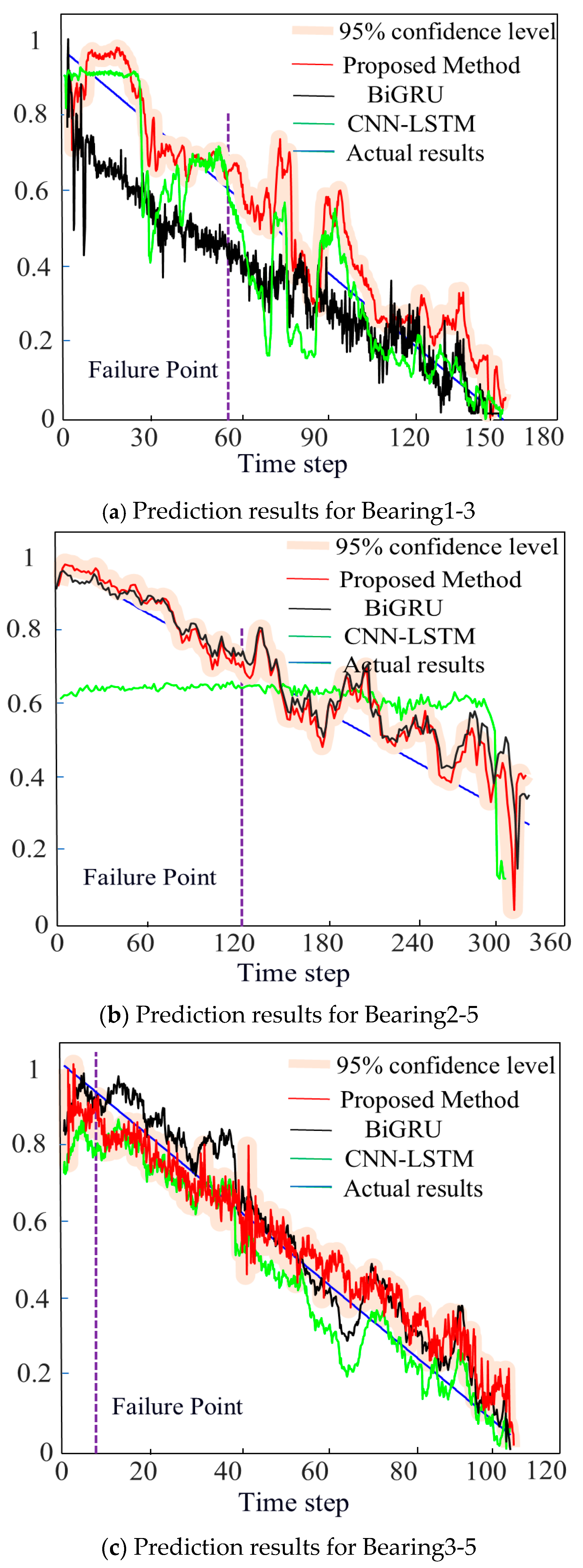
When establishing a network model that combines a Double-way Bidirectional Long Short-Term Memory network with an attention mechanism for predicting the RUL of bearings, when tested with the datasets Bearing1-3, Bearing2-6, and Bearing3-3 from PHM2012, the p-values between the prediction results of the proposed RUL method and those of the BiGRU prediction method are 0.0188, 0.0012, and 0.0234, respectively; the p-values between the prediction results of the proposed RUL method and those of the CNN-LSTM prediction method are also 0.0188, 0.0012, and 0.0234, respectively, with p < 0.05. When tested with the datasets Bearing1-3, Bearing2-5, and Bearing3-5 from XJTU-SY, the p-values between the prediction results of the proposed RUL method and those of the BiGRU prediction method are 0.0196, 0.0012, and 0.0241, respectively; the p-values between the prediction results of the proposed RUL method and those of the CNN-LSTM prediction method are 0.0001, 0.0083, and 0.0327, respectively, with p < 0.05. The prediction results from both datasets can demonstrate significant differences between the proposed method and the comparative methods. Therefore, the RUL prediction performance of the proposed method is higher. Moreover, the prediction curves for both datasets fall within the 95% confidence interval, which demonstrates the reliability of the prediction results obtained using the proposed model.

(4)

When compared with the BiGRU (Bidirectional Gated Recurrent Neural Network) method and the CNN-LSTM (Hybrid Model of Convolutional Neural Network and LSTM Network) method, the proposed prediction model, when validated using the PHM2012 dataset and the XJTU-SY dataset, yielded smaller RMSE and MAE values in the prediction results (Table 8 and Table 10) than the other two comparative methods. Although the other two methods could also predict RUL results, the RUL curves exhibited greater fluctuations. Generally speaking, smaller RMSE and MAE values indicate better model performance. The R² value of the proposed prediction model is closer to 1, and the model’s fitting ability is also superior to that of the comparative methods. Therefore, the proposed model further enhances the performance of RUL prediction. Additionally, this also demonstrates that the proposed prediction model is less influenced by data variations and possesses strong generalization capabilities and practicality.

(5)

The proposed method performs well under different operating conditions and across various datasets; therefore the proposed method demonstrates higher effectiveness in predicting RUL. By employing this method for RUL prediction, potential bearing failures can be detected in a timely manner, providing sufficient time to prompt bearing repairs. It guides personnel in formulating comprehensive maintenance strategies, thereby preventing further deterioration of faults that could lead to equipment shutdown or damage, and reducing economic losses caused by fault-induced downtime.

References

1. Shang, J.; Xu, D.; Qiu, H.; Jiang, C.; Gao, L. Domain generalization for rotating machinery real-time remaining useful life prediction via multi-domain orthogonal degradation feature exploration. Mech. Syst. Signal Process. 2025, 223, 111924. [Google Scholar] [CrossRef]
2. Sun, Y.; Wang, Z. Remaining useful life prediction of rolling bearing via composite multiscale permutation entropy and Elman neural network. Eng. Appl. Artif. Intell. 2024, 135, 108852. [Google Scholar] [CrossRef]
3. Xu, Z.; Zhang, Y.; Miao, Q. An attention-based Multi-Scale Temporal Convolutional Network for Remaining Useful Life Prediction. Reliab. Eng. Syst. Saf. 2024, 250, 110288. [Google Scholar] [CrossRef]
4. Chen, K.; Liu, J.; Guo, W.; Wang, X. A two-stage approach based on Bayesian deep learning for predicting remaining useful life of rolling element bearings. Comput. Electr. Eng. 2023, 109, 108745. [Google Scholar] [CrossRef]
5. Cui, L.; Xiao, Y.; Liu, D.; Han, H. Digital twin-driven graph domain adaptation neural network for remaining useful life prediction of rolling bearing. Reliab. Eng. Syst. Saf. 2024, 245, 109991. [Google Scholar] [CrossRef]
6. Saidi, L.; Ali, J.B.; Bechhoefer, E.; Benbouzid, M. Wind turbine high-speed shaft bearings health prognosis through a spectral Kurtosis-derived indices and SVR. Appl. Acoust. 2017, 120, 1–8. [Google Scholar] [CrossRef]
7. Li, Q.; Yan, C.; Chen, G.; Wang, H.; Li, H.; Wu, L. Remaining Useful Life prediction of rolling bearings based on risk assessment and degradation state coefficient. ISA Trans. 2022, 129, 413–428. [Google Scholar] [CrossRef]
8. Qin, Y.; Chen, D.; Xiang, S.; Zhu, C. Gated dual attention unit neural networks for remaining useful life prediction of rolling bearings. IEEE Trans. Ind. Inform. 2020, 17, 6438–6447. [Google Scholar] [CrossRef]
9. Tang, G.; Liu, L.; Liu, Y.; Yi, C.; Hu, Y.; Xu, D.; Zhou, Q.; Lin, J. Unsupervised transfer learning for intelligent health status identification of bearing in adaptive input length selection. Eng. Appl. Artif. Intell. 2023, 126, 107051. [Google Scholar] [CrossRef]
10. Wu, J.; Hu, K.; Cheng, Y.; Zhu, H.; Shao, X.; Wang, Y. Data-driven remaining useful life prediction via multiple sensor signals and deep long short-term memory neural network. ISA Trans. 2020, 97, 241–250. [Google Scholar] [CrossRef]
11. Yu, W.; Shao, Y.; Xu, J.; Mechefske, C. An adaptive and generalized Wiener process model with a recursive filtering algorithm for remaining useful life estimation. Reliab. Eng. Syst. Saf. 2022, 217, 108099. [Google Scholar] [CrossRef]
12. Lin, J.; Liao, G.; Chen, M.; Yin, H. Two-phase degradation modeling and remaining useful life prediction using nonlinear wiener process. Comput. Ind. Eng. 2021, 160, 107533. [Google Scholar] [CrossRef]
13. Duan, F.; Wang, G. Bayesian analysis for the transformed exponential dispersion process with random effects. Reliab. Eng. Syst. Saf. 2022, 217, 108104. [Google Scholar] [CrossRef]
14. Que, Z.; Jin, X.; Xu, Z. Remaining useful life prediction for bearings based on a gated recurrent unit. IEEE Trans. Instrum. Meas. 2021, 70, 3511411. [Google Scholar] [CrossRef]
15. Berghout, T.; Mouss, L.-H.; Kadri, O.; Saïdi, L.; Benbouzid, M. Aircraft engines Remaining Useful Life prediction with an adaptive denoising online sequential Extreme Learning Machine. Eng. Appl. Artif. Intell. 2020, 96, 103936. [Google Scholar] [CrossRef]
16. Xu, M.; Wang, J.; Liu, J.; Li, M.; Geng, J.; Wu, Y.; Song, Z. An improved hybrid modeling method based on extreme learning machine for gas turbine engine. Aerosp. Sci. Technol. 2020, 107, 106333. [Google Scholar] [CrossRef]
17. Elforjani, M.; Shanbr, S. Prognosis of bearing acoustic emission signals using supervised machine learning. IEEE Trans. Ind. Electron. 2017, 65, 5864–5871. [Google Scholar] [CrossRef]
18. Xie, G.; Jia, H.; Li, H.; Zhong, Y.; Du, W.; Dong, Y.; Wang, L.; Lv, J. A life prediction method of mechanical structures based on the phase field method and neural network. Appl. Math. Model. 2023, 119, 782–802. [Google Scholar] [CrossRef]
19. Kankar, P.K.; Sharma, S.C.; Harsha, S.P. Vibration-based fault diagnosis of a rotor bearing system using artificial neural network and support vector machine. Int. J. Model. Ident. Control 2012, 15, 185–198. [Google Scholar] [CrossRef]
20. Shi, L.; Su, S.; Wang, W.; Gao, S.; Chu, C. Bearing Fault Diagnosis Method Based on Deep Learning and Health State Division. Appl. Sci. 2023, 13, 7424. [Google Scholar] [CrossRef]
21. Niu, G.; Wang, X.; Liu, E.; Zhang, B. Lebesgue sampling based deep belief network for lithium-ion battery diagnosis and prognosis. IEEE Trans. Ind. Electron. 2021, 69, 8481–8490. [Google Scholar] [CrossRef]
22. Qin, Y.; Wang, X.; Zou, J. The optimized deep belief networks with improved logistic sigmoid units and their application in fault diagnosis for planetary gearboxes of wind turbines. IEEE Trans. Ind. Electron. 2018, 66, 3814–3824. [Google Scholar] [CrossRef]
23. Qiu, H.; Niu, Y.; Shang, J.; Gao, L.; Xu, D. A piecewise method for bearing remaining useful life estimation using temporal convolutional networks. J. Manuf. Syst. 2023, 68, 227–241. [Google Scholar] [CrossRef]
24. Mo, H.; Custode, L.L.; Iacca, G. Evolutionary neural architecture search for remaining useful life prediction. Appl. Soft Comput. 2021, 108, 107474. [Google Scholar] [CrossRef]
25. Xia, M.; Zheng, X.; Imran, M.; Shoaib, M. Data-driven prognosis method using hybrid deep recurrent neural network. Appl. Soft Comput. 2020, 93, 106351. [Google Scholar] [CrossRef]
26. Zhang, H.; Xi, X.; Pan, R. A two-stage data-driven approach to remaining useful life prediction via long short-term memory networks. Reliab. Eng. Syst. Saf. 2023, 237, 109332. [Google Scholar] [CrossRef]
27. Ni, Q.; Ji, J.C.; Feng, K. Data-driven prognostic scheme for bearings based on a novel health indicator and gated recurrent unit network. IEEE Trans. Ind. Inform. 2022, 19, 1301–1311. [Google Scholar] [CrossRef]
28. Yang, X.; Zheng, Y.; Zhang, Y.; Wong, D.S.-H.; Yang, W. Bearing remaining useful life prediction based on regression shapalet and graph neural network. IEEE Trans. Instrum. Meas. 2022, 71, 3505712. [Google Scholar] [CrossRef]
29. Shang, X.; Li, W.; Yuan, F.; Zhi, H.; Gao, Z.; Guo, M.; Xin, B. Research on Fault Diagnosis of UAV Rotor Motor Bearings Based on WPT-CEEMD-CNN-LSTM. Machines 2025, 13, 287. [Google Scholar] [CrossRef]
30. Matania, O.; Bachar, L.; Bechhoefer, E.; Bortman, J. Signal Processing for the Condition-Based Maintenance of Rotating Machines via Vibration Analysis: A Tutorial. Sensors 2024, 24, 454. [Google Scholar] [CrossRef]
31. Randall, R.B. Vibration-Based Condition Monitoring: Industrial, Aerospace and Automotive Applications; John Wiley & Sons: Chichester, UK, 2011. [Google Scholar]
32. Wu, Y.; Dai, J.; Yang, X.; Shao, F.; Gong, J.; Zhang, P.; Liu, S. The Fault Diagnosis of Rolling Bearings Based on FFT-SE-TCN-SVM. Actuators 2025, 14, 152. [Google Scholar] [CrossRef]
33. Li, T.; Zhou, Z.; Li, S.; Sun, C.; Yan, R.; Chen, X. The emerging graph neural networks for intelligent fault diagnostics and prognostics: A guideline and a benchmark study. Mech. Syst. Signal Process. 2022, 168, 108653. [Google Scholar] [CrossRef]
34. Yang, C.; Ma, J.; Wang, X.; Li, X.; Li, Z.; Luo, T. A novel based-performance degradation indicator remaining useful life prediction model and its application in rolling bearing. ISA Trans. 2022, 121, 349–364. [Google Scholar] [CrossRef]
35. Kumar, P.S.; Kumaraswamidhas, L.; Laha, S. Selection of efficient degradation features for rolling element bearing prognosis using Gaussian Process Regression method. ISA Trans. 2020, 112, 386–401. [Google Scholar] [CrossRef] [PubMed]
36. Qi, J.; Zhu, R.; Liu, C.; Mauricio, A.; Gryllias, K. Anomaly detection and multi-step estimation based remaining useful life prediction for rolling element bearings. Mech. Syst. Signal Process. 2024, 206, 110910. [Google Scholar] [CrossRef]
37. Li, X.; Teng, W.; Peng, D.; Ma, T.; Wu, X.; Liu, Y. Feature fusion model based health indicator construction and self-constraint state-space estimator for remaining useful life prediction of bearings in wind turbines. Reliab. Eng. Syst. Saf. 2023, 233, 109124. [Google Scholar] [CrossRef]
38. Lu, Q.; Li, M. Digital Twin-Driven Remaining Useful Life Prediction for Rolling Element Bearing. Machines 2023, 11, 678. [Google Scholar] [CrossRef]
39. Li, J.; Huang, F.; Qin, H.; Pan, J. Research on Remaining Useful Life Prediction of Bearings Based on MBCNN-BiLSTM. Appl. Sci. 2023, 13, 7706. [Google Scholar] [CrossRef]
40. Fan, Z.; Li, W.; Chang, K.-C. A Bidirectional Long Short-Term Memory Autoencoder Transformer for Remaining Useful Life Estimation. Mathematics 2023, 11, 4972. [Google Scholar] [CrossRef]
41. Wang, L.; Zhu, Z.; Zhao, X. Dynamic predictive maintenance strategy for system remaining useful life prediction via deep learning ensemble method. Reliab. Eng. Syst. Saf. 2024, 245, 110012. [Google Scholar] [CrossRef]
42. Gan, F.; Qin, Y.; Xia, B.; Mi, D.; Zhang, L. Remaining useful life prediction of aero-engine via temporal convolutional network with gated convolution and channel selection unit. Appl. Soft Comput. 2024, 167, 112325. [Google Scholar] [CrossRef]
43. Zhao, X.; Yang, Y.; Huang, Q.; Fu, Q.; Wang, R.; Wang, L. Rolling bearing remaining useful life prediction method based on vibration signal and mechanism model. Appl. Acoust. 2025, 228, 110334. [Google Scholar] [CrossRef]
44. Rathore, M.S.; Harsha, S. An attention-based stacked BiLSTM framework for predicting remaining useful life of rolling bearings. Appl. Soft Comput. 2022, 131, 109765. [Google Scholar] [CrossRef]
45. Shang, Y.; Tang, X.; Zhao, G.; Jiang, P.; Lin, T.R. A remaining life prediction of rolling element bearings based on a bidirectional gate recurrent unit and convolution neural network. Measurement 2022, 202, 111893. [Google Scholar] [CrossRef]
46. Jiang, L.; Zhang, T.; Lei, W.; Zhuang, K.; Li, Y. A new convolutional dual-channel Transformer network with time window concatenation for remaining useful life prediction of rolling bearings. Adv. Eng. Inform. 2023, 56, 101966. [Google Scholar] [CrossRef]
47. Guo, K.; Ma, J.; Wu, J.; Xiong, X. Adaptive feature fusion and disturbance correction for accurate remaining useful life prediction of rolling bearings. Eng. Appl. Artif. Intell. 2024, 138, 109433. [Google Scholar] [CrossRef]
48. Li, N.; Lei, Y.; Lin, J.; Ding, S.X. An improved exponential model for predicting remaining useful life of rolling element bearings. IEEE Trans. Ind. Electron. 2015, 62, 7762–7773. [Google Scholar] [CrossRef]
49. Wang, Y.; Peng, Y.; Zi, Y.; Jin, X.; Tsui, K.-L. A two-stage data-driven-based prognostic approach for bearing degradation problem. IEEE Trans. Ind. Inform. 2016, 12, 924–932. [Google Scholar] [CrossRef]
50. Wen, J.; Gao, H.; Zhang, J. Bearing remaining useful life prediction based on a nonlinear wiener process model. Shock. Vib. 2018, 2018, 4068431. [Google Scholar] [CrossRef]
51. Wang, H.; Zhao, Y.; Ma, X. Remaining useful life prediction using a novel two-stage wiener process with stage correlation. IEEE Access 2018, 6, 65227–65238. [Google Scholar] [CrossRef]
52. Wang, D.; Tsui, K.-L. Two novel mixed effects models for prognostics of rolling element bearings. Mech. Syst. Signal Process. 2018, 99, 1–13. [Google Scholar] [CrossRef]
53. Li, J.; Fan, J.; Wang, Z.; Qiu, M.; Liu, X. A new method for change-point identification and RUL prediction of rolling bearings using SIC and incremental Kalman filtering. Measurement 2025, 250, 117150. [Google Scholar] [CrossRef]
54. Matania, O.; Cohen, R.; Bechhoefer, E.; Bortman, J. Zero-fault-shot learning for bearing spall type classification by hybrid approach. Mech. Syst. Signal Process. 2025, 224, 112117. [Google Scholar] [CrossRef]
55. Sheng, Z. Probability Theory and Mathematical Statistics, 3rd ed.; Higher Education Press: Beijing, China, 2001. [Google Scholar]
Figure 1. Overall technical roadmap.
Applsci 15 04441 g001
Figure 2. Wavelet decomposition principle.
Applsci 15 04441 g002
Figure 3. Memory cell of LSTM network.
Applsci 15 04441 g003
Figure 4. Working principle of double BiLSTM (DBiLSTM).
Applsci 15 04441 g004
Figure 5. Attention mechanism network structure.
Applsci 15 04441 g005
Figure 6. Network structure of A-DBiLSTM.
Applsci 15 04441 g006
Figure 7. Data acquisition platform.
Applsci 15 04441 g007
Figure 8. Denoising result.
Applsci 15 04441 g008
Figure 9. Feature maps.
Applsci 15 04441 g009
Figure 10. Ranking of weighted averages corresponding to different features.
Applsci 15 04441 g010
Figure 11. Selected feature indicators.
Applsci 15 04441 g011
Figure 12. Health indicator and failure threshold.
Applsci 15 04441 g012
Figure 13. The results of the RUL.
Applsci 15 04441 g013
Figure 14. The results of the RUL.
Applsci 15 04441 g014