BoxRF: A New Machine Learning Algorithm for Grade Estimation

Abstract

A new machine learning algorithm, BoxRF, was developed specifically for estimating grades from drillhole datasets. The method combines the features of classical estimation methods, such as search boxes, search direction, and estimation based on inverse distance methods, with the robustness of random forest (RF) methods that come from forming numerous random groups of data. The method was applied to a porphyry copper deposit, and results were compared to various ML methods, including XGBoost (XGB), k-nearest neighbors (KNN), neural nets (NN), and RF. Scikit-learn RF (SRF) performed the best (R² = 0.696) among the ML methods but underperformed BoxRF (R² = 0.751). The results were confirmed through a five-fold cross-validation exercise where BoxRF once again outperformed SRF. The box dimensions that performed the best were similar in length to the ranges indicated by variogram modeling, thus demonstrating a link between machine learning and traditional methods. Numerous combinations of hyperparameters performed similarly well, implying the method is robust. The inverse distance method was found to better represent the grade–space relationship in BoxRF than median values. The superiority of BoxRF over SRF in this dataset is encouraging, as it opens the possibility of improving machine learning by incorporating domain knowledge (principles of geology, in this case).

1. Introduction

Grade estimation and orebody modeling are important elements of mining, whether it is at the exploration/mine development stage or at the operational stage. While geostatistics has traditionally been the key technique used for orebody modeling, artificial intelligence (AI) methods have been examined by researchers in the last two or three decades in a wide variety of deposits [1,2,3,4,5,6]. Documented AI performances have been all over the place, from marginal to inferior to geostatistics, to better than geostatistics [6,7,8,9,10]. The appeal for AI has always been that specialized skills are less important than in geostatistics [1]. Therefore, from the very beginning, researchers tested this assumption. Issues such as sparseness in data, the effect of data aggregation, and subdivision methods for training/testing were investigated [11,12] to understand how these components affected prediction performance.

As research on the use of AI in mining has matured, researchers have focused on addressing the limitations of geostatistics by manipulating AI modeling methods or using geostatistics to gain insights into AI performance [13]. Variogram ranges were found to be insightful concerning hyperparameter selection in AI modeling, as well as serving as indicators of AI model performance [14]. A method that combined kriging and random forests (RFs) was reported to have performance that was superior to both methods in modeling aboveground biomass [15]. The researchers did not change the methods themselves; the two methods were applied sequentially, though not like an ensemble. Some researchers combined SVM with heuristic reasoning to create geologically realistic domain boundaries [5], while others just combined geostatistics and machine learning models using an ensemble approach [16]. None of the geostatistics–AI combinations involved changing AI methods structurally, however. The researchers were simply creative about what data were fed to the methods [17]. This is also true of other (non-grade estimation) AI geospatial applications [18,19,20] where the focus was on the importance of applications and the use of big data. “Big data” applies to the broader geospatial sector, as data are typically generated by sensors (satellite, aerial campaigns), whereas it does not apply to mining drillhole datasets, as they are limited in quantity, as drilling is expensive. Therefore, some geospatial modelers modify AI methods by imposing the use of important covariates as inputs along with distances [21]. Some also suggested transfer learning, where knowledge from one area was used to model another [17,22]. Those not involving image processing focused on neural networks, random forests, support vector machines, and boosted methods [23].

A recently published approach, GeoRF, however, has made structural changes to the RF method by modifying how samples are split [24]. This research, which reported superior results to the typical RF, was contemporaneous with the work being performed for this paper. Rather than a split based on a single variable, they based the split based on multiple variables.

In a step that significantly advances the enmeshing of geostatistical methods and AI, this paper announces a new AI method that is created through structural changes made to the RF method. This method is called BoxRF to acknowledge that the proposed RF type method was developed by applying the concept of search boxes typical in orebody modeling. There are several differences between GeoRF and BoxRF. The biggest differences are that BoxRF splits are in 3D boxes, and directions are very important. BoxRF actively looks for trends. BoxRF also makes multivariate splits, but the split criteria are different. BoxRF also incorporates strategies to improve predictions by accommodating the challenges of mining industry drillhole datasets. The method of prediction from a split is also different. Drillhole datasets are different from geospatial geographical datasets; usually, the latter is data-rich, as the data are from satellite and sensors. Therefore, the geospatial modeling strategies (RF or not) recommended in the literature [21,24,25] may not work for modeling drillhole datasets. It was important, therefore, for the authors of this paper to explore the link between BoxRF and established concepts that are easily understood.

Thus, the biggest impact of the proposed method is not the improved results, but the trust it engenders in AI, as its performance is linked to concepts such as variograms that are intuitively understandable. Since the proposed method is not about creatively feeding data into existing tools, the method was programmed from scratch in Python.

2. Materials and Methods

The proposed technique has its basis in the structure of RFs. Readers unfamiliar with RFs are referred to [2], an open-source publication that presents RFs in a way that is relevant to this paper. At its essence, RFs employ a set of samples, known as leaves, to make predictions. These leaves are produced through a random and sequential division of data. By segmenting the data in numerous different ways, a series of divisions culminates in a collection of leaves, called trees. In the BoxRF method, leaves are a random set of “boxes”, with a box being a 3D region in space. The dimension of the boxes is set by the user based on their knowledge of the deposit. The dimensions are not fixed; they are set as ranges based on expected lengths of geological trends. The intention behind the use of boxes is to capture trends, like how they are used as search boxes in classical reserve estimation methods. In the classical methods, search boxes are typically fixed in dimension and direction, whereas in the BoxRF method, they are not.

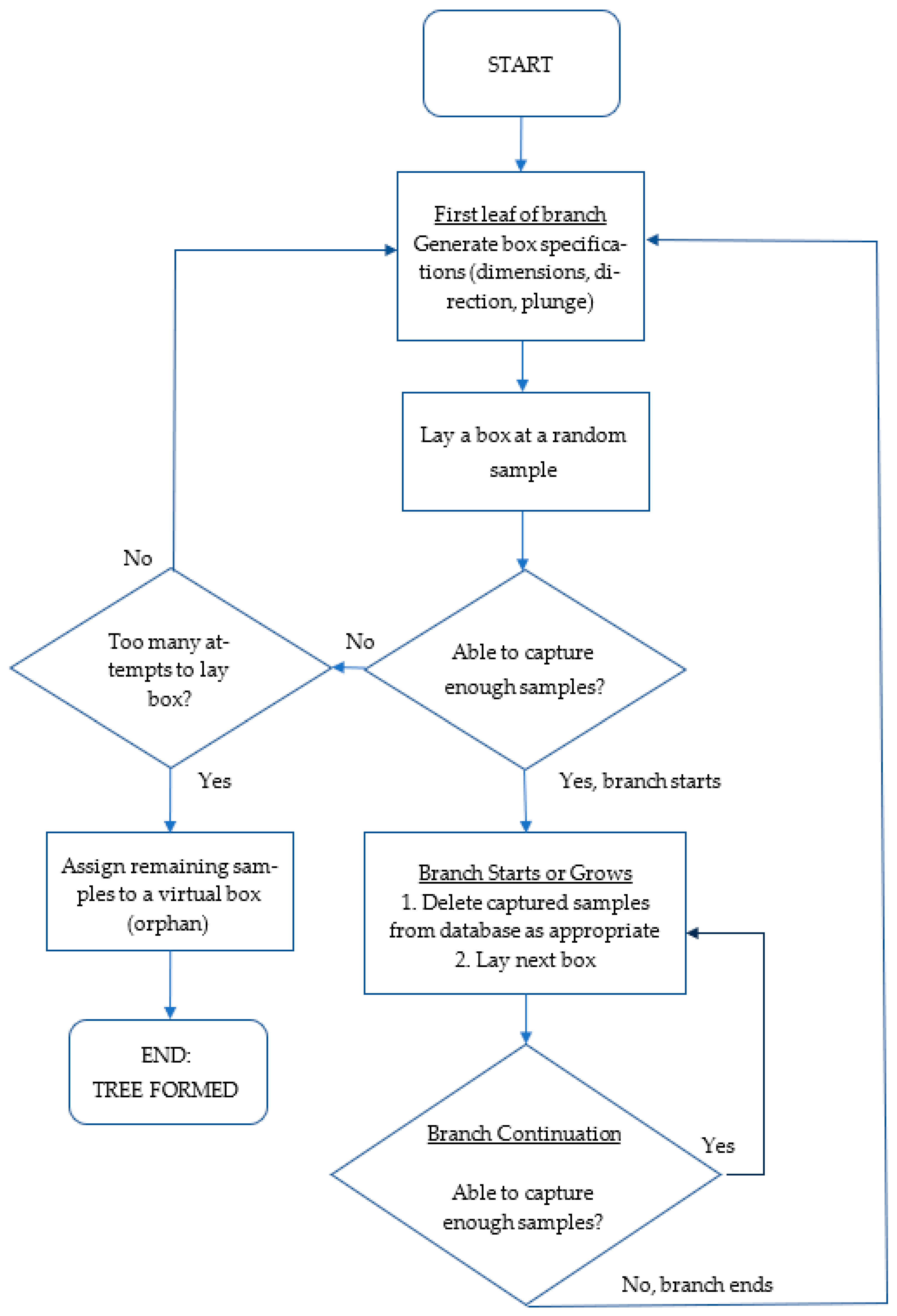
The BoxRF method starts with laying a box at the location of a randomly selected sample (Figure 1). The direction and plunge of the box are randomly determined. Once a box is generated, all samples that fall within the box are identified. If the number of samples in a box meets a threshold (minimum samples in a box or MS), the box is “accepted” and the samples inside the box are deleted from the database. There is a nuance about the deletion of samples that is discussed in a subsequent section. This is reflected in Figure 1 as “Delete captured samples from database as appropriate”. The next box is then laid at the end of the current box, so that it is in the same alignment as the current box. The next box has the same dimensions as the current one. The logic is to continue laying boxes in a random direction as long as the MS requirements are met.

When two or more boxes are laid in sequence, the structure is called a branch (though a branch may have just one box eventually). The process stops when a box is rejected for having insufficient samples. A new box is then generated at the location of a randomly selected sample with a different dimension and in a different direction. The process continues until boxes cannot be formed. Twenty-five attempts are made to form boxes before the process is stopped. At the end of the process, there will always be a sprinkling of samples that are not in any boxes. These orphan samples are treated as a leaf and represent the region outside of all the boxes (“orphan leaf”). The collection of boxes, along with the orphan leaf, is called a tree (Figure 2). Like RFs, the BoxRF method requires several trees. Once a tree is formed, the algorithm continues to generate the next tree with a fresh copy of the dataset.

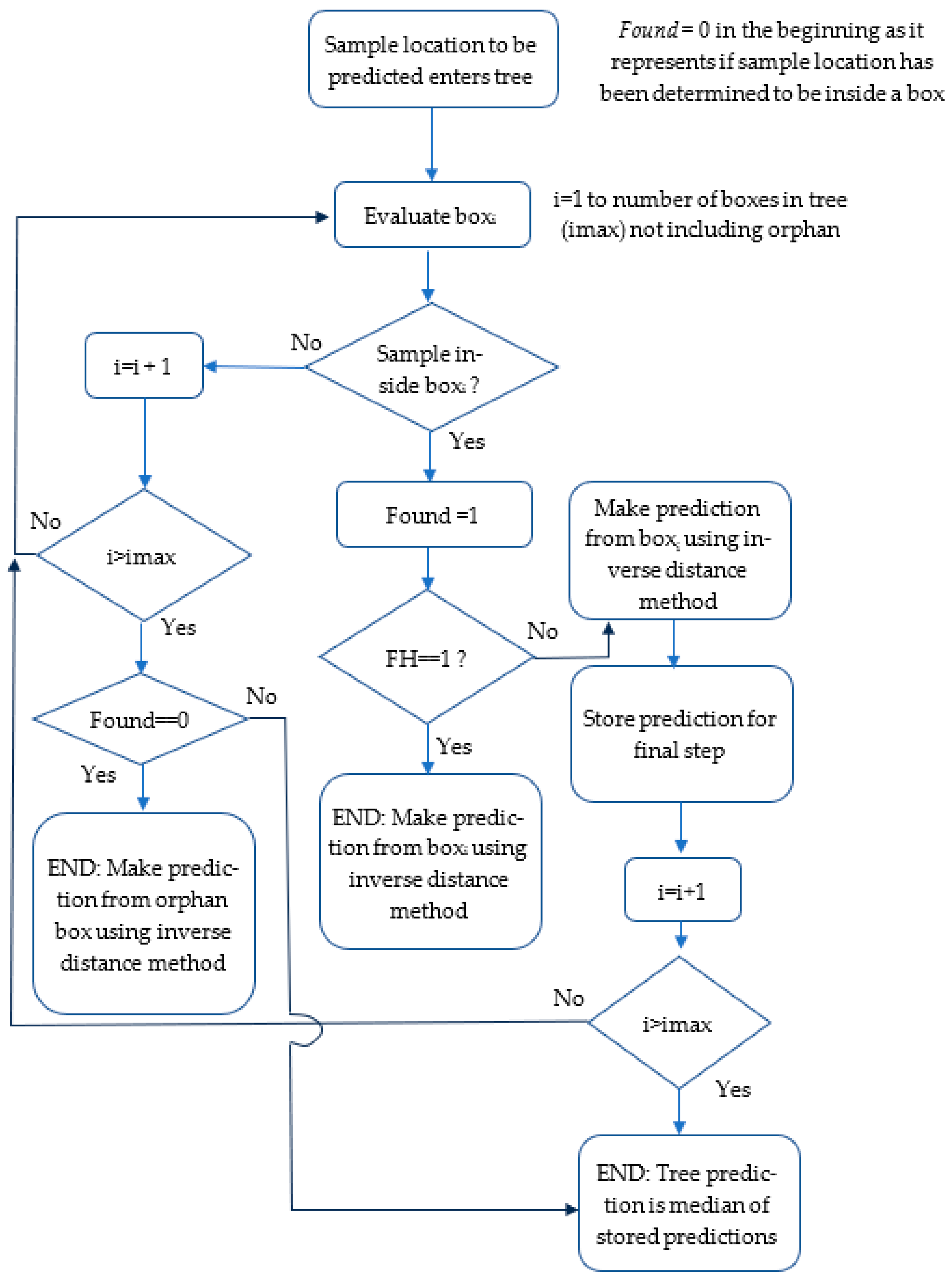
After the RF is formed, it is used to make predictions. The final similarity and difference between RF and BoxRF are in how predictions are made. Two flowcharts are provided in subsequent sections to help describe the prediction method. In both methods, the final prediction is obtained from the predictions made by individual trees. RFs typically obtain the final prediction by taking the mean or median of predictions made by individual trees. In RFs, a prediction is made by a tree from a leaf that represents the prediction location most closely. In BoxRF, a prediction is made by the box whose space includes the location to be predicted. When a sample is outside any of the boxes in a tree, a prediction is made from the orphan leaf. In an RF, the prediction from a leaf is simply the mean or median of the samples in the leaf. The BoxRF method, on the other hand, uses the inverse distance (ID) method on the samples contained in the leaf to obtain the prediction. Thus, the BoxRF method honors the classical techniques by giving more weight to nearby samples. In this paper, the ID method was used with a power of 3, as it was found to perform better.

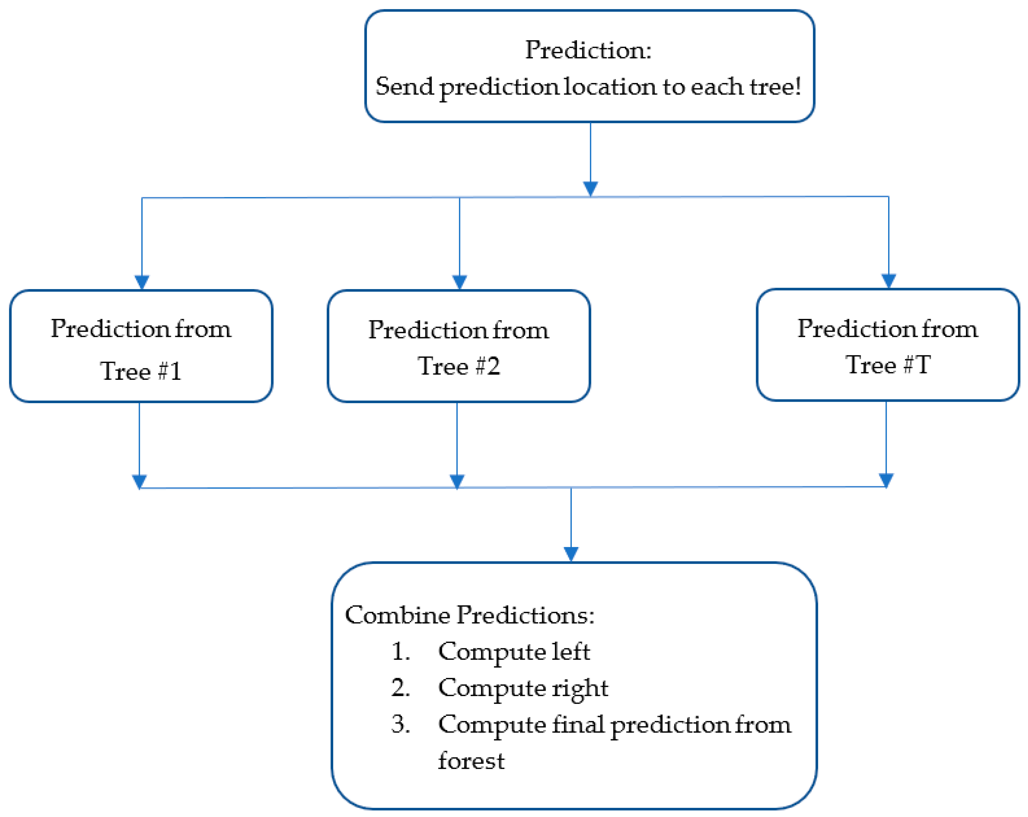
The BoxRF method also combines tree predictions differently than classical RFs (Figure 3). Rather than take the mean or median of tree predictions as the final prediction, it first determines whether the collection of predictions from the trees is skewed or not. Then, it determines the final prediction as follows:

Left = prediction₅₀ − prediction₁₀;

(1)

where prediction_p is prediction at the pth percentile.

Right = prediction₉₀ − prediction₅₀

(2)

If (left/right) > 5, predictions are right-skewed, as most predictions are higher than the median prediction.

If (right/left) > 5, predictions are left-skewed; i.e., most predictions fall between the median value and the lowest value.

If the skew is neither left nor right, predictions are not skewed.

The final prediction is as follows:

prediction50	if predictions are not skewed;
0.5× (prediction10 + prediction50)	if predictions are left-skewed;
0.5× (prediction50 + prediction90)	if predictions are right-skewed.

2.1. Nuances of the Method

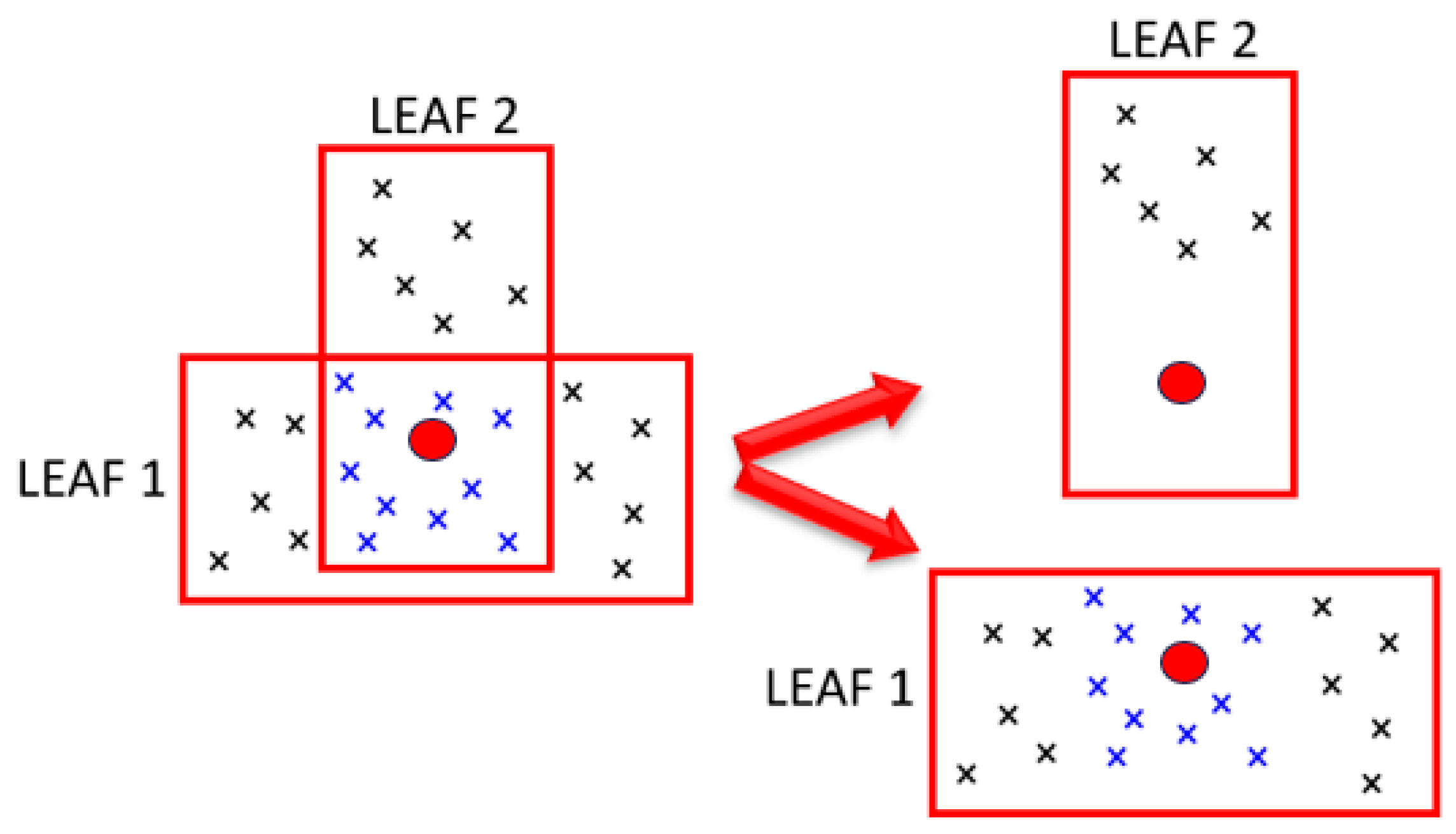
Since boxes (or leaves) are formed randomly, two leaves in the same tree may represent overlapping regions. This is shown in Figure 4. Assuming Leaf 1 is formed first, all the samples within it are unavailable when Leaf 2 forms. Thus, Leaf 2 only has samples at one end as it does not have access to the blue samples that fall within its region, making Leaf 2 not very representative of its space. The lack of representativeness creates an issue when the dark red point, which falls within both leaves, is to be predicted. Both leaves claim the sample location, but clearly, the prediction from Leaf 2 is problematic for the red location, as it contains no samples that span the red location.

This situation is dealt with using the hyperparameter number of times to reuse samples (NR). When NR = 1, a sample is deleted from the database once it is inside a leaf. When NR = 2, the sample is allowed to be claimed by two leaves before it is deleted from the database. This minimizes the occurrence of the situations described previously. The deletion of samples is essential, as otherwise, leaf formation will not stop. Also, if samples are not deleted after being claimed by a leaf, too many leaves represent a region, and a legitimate trend contained within a leaf becomes diluted by the presence of other leaves. Therefore, NR was only tested with values of 1 and 2.

The BoxRF method contains another nuance. What is the prediction from the tree when multiple leaves within it are allowed to make predictions for a given location? In this paper, this issue was tested through a hyperparameter called predict from first hit only (FH). When a location is to be predicted, the tree scrolls through the leaves to determine leaves that can claim the location and make the prediction. When FH = 1, the prediction of the tree comes from the first leaf that is found to contain the prediction location (Figure 5). When FH = 2, the tree prediction is the median of predictions from the various leaves that claim the location.

2.2. Modeling Details

The data used for this paper come from the Erdenet copper mine in Mongolia. Details about the deposit are available in both the public domain [3] and in a doctoral dissertation [26]. The dataset, consisting of over two thousand exploration drillholes, represents two deposits in the mine. Each row in the database represented a 5 m thick drillhole interval and consisted of the three coordinates of the interval location and the copper grade (in percentage). There are 90,033 rows in the database. The modeling in the paper was aimed at predicting the copper grade for a given set of coordinates.

Previous variogram modeling [26] on copper grades had shown variograms to have a high nugget component, and a range of 100–200 m. In that work, the two deposits in the mine were modeled separately, unlike in this paper. In many directions, the models were purely nugget models. Pure nugget models suggest an infinite range since the data are purely random. Using this as information, 12 combinations of box dimensions were attempted (

Table 1. Box dimensions used to create leaves.

Box Dimension	Dimension Combinations
Box Length (BL)	[50, 100], [100, 300], [300, 500]
Box Width (BW)	[50, 100], [100, 200]
Box Height (BH)	[25, 50], [50, 100], [100, 300]

). Box dimensions are specified as ranges in meters. Thus, a dimension of [50, 100] for box length instructs BoxRF to generate boxes of length between 50 m and 100 m.

Other hyperparameters of the algorithm and their options are shown in

Table 2. Hyperparameter settings.

Hyperparameter	Values
Prediction from first hit only (FH)	1, 2
Number of times to reuse sample (NR)	1, 2
Number of trees (T)	3, 7, 11, 15
Minimum number of samples in a box (MS)	3, 5

:

The dataset was split into training (70%) and testing (30%) subsets. Splitting was carried out in such a way as to ensure the subsets were similar.

Table 3. Similarity of training and testing subsets.

Percentile	Column	Train	Test
10	East	435,431	435,430
	North	5,428,712	5,428,719
	Elevation	1017	1012
	Grade	0.04	0.04
25	East	435,874	435,874
	North	5,429,580	5,429,577
	Elevation	1161	1160
	Grade	0.13	0.14
50	East	436,464	436,464
	North	5,430,148	5,430,151
	Elevation	1303	1302
	Grade	0.32	0.32
75	East	436,940	436,940
	North	5,430,536	5,430,533
	Elevation	1385	1385
	Grade	0.54	0.55
90	East	437,695	437,693
	North	5,430,818	5,430,817
	Elevation	1423	1423
	Grade	0.80	0.80

shows the similarity between the train and test subsets at various percentiles.

3. Results

The top 5 performances of the four combinations—(NR = 1, FH = 1), (NR = 1, FH = 2), (NR = 2, FH = 1), and (NR = 2, FH = 2)—are shown in

Table 4. Top 5 performances for NR = 1, FH = 1.

R2	R2_std	RMSE	RMSE_std	BL	BW	BH	MS	T
0.751	0.000	0.170	0.000	[100, 300]	[100, 200]	[50, 100]	5	11
0.750	0.001	0.170	0.000	[100, 300]	[50, 100]	[50, 100]	5	9
0.750	0.001	0.170	0.000	[100, 300]	[50, 100]	[50, 100]	3	11
0.750	0.000	0.170	0.000	[100, 300]	[100, 200]	[50, 100]	3	9
0.750	0.000	0.170	0.000	[100, 300]	[100, 200]	[50, 100]	3	11

,

Table 5. Top 5 performances for NR = 1, FH = 2.

R2	R2_std	RMSE	RMSE_std	BL	BW	BH	MS	T
0.739	0.003	0.174	0.001	[50, 100]	[50, 100]	[50, 100]	3	11
0.735	0.003	0.175	0.001	[50, 100]	[50, 100]	[50, 100]	5	7
0.732	0.003	0.176	0.001	[50, 100]	[50, 100]	[50, 100]	3	7
0.717	0.006	0.181	0.002	[50, 100]	[50, 100]	[50, 100]	3	3
0.711	0.006	0.183	0.002	[50, 100]	[50, 100]	[50, 100]	5	3

,

Table 6. Top 5 performances for NR = 2, FH = 1.

R2	R2_std	RMSE	RMSE_std	BL	BW	BH	MS	T
0.751	0.000	0.170	0.000	[50, 100]	[50, 100]	[100, 300]	3	11
0.751	0.000	0.170	0.000	[50, 100]	[50, 100]	[50, 100]	3	11
0.751	0.000	0.170	0.000	[100, 300]	[50, 100]	[100, 300]	3	11
0.750	0.000	0.170	0.000	[100, 300]	[100, 200]	[50, 100]	3	7
0.750	0.000	0.170	0.000	[300, 500]	[50, 100]	[100, 300]	3	11

and

Table 7. Top 5 performances for NR = 2, FH = 2.

R2	R2_std	RMSE	RMSE_std	BL	BW	BH	MS	T
0.749	0.001	0.170	0.000	[50, 100]	[50, 100]	[50, 100]	3	11
0.744	0.002	0.172	0.001	[100, 300]	[50, 100]	[25, 50]	5	9
0.744	0.003	0.172	0.001	[100, 300]	[50, 100]	[25, 50]	5	11
0.744	0.002	0.172	0.001	[100, 300]	[50, 100]	[25, 50]	5	9
0.743	0.003	0.173	0.001	[100, 300]	[50, 100]	[50, 100]	5	11

. The performances shown are R² (coefficient of determination), R²_std, root mean square error (RMSE), RMSE_std, box dimensions, minimum number of samples in the box, and the number of trees. Each row of the tables represents median performance across seven iterations with the listed hyperparameters. R²_std is the standard deviation of R² across the seven iterations. This was computed to determine if the performances varied significantly from one random iteration to the next. RMSE_std similarly shows the standard deviation for the RMSE.

Several things are observed:

• The median R² performance is 0.75, which is almost identical to the best performance. This means that several combinations can yield a high performance.
• The performances are tightly clustered around R² of 0.71 to 0.75, with NR = 1 and FH = 2 underperforming the most. This underperformance is not surprising, as NR =1 can result in boxes not populating well, while FH = 2 forces predictions to consider all boxes that contain the location to be predicted.
• The standard deviations for both R² and RMSE are very low, suggesting that random iterations did not yield very different performances. In other words, for a given set of hyperparameters, BoxRF produces consistent results.
• The top 50% of the reported highest performances had 11 trees. Except for one, all had a minimum sample size of three. No top-performing model had 15 trees.
• Out of the 20 results shown, 12 of them contain 11 trees, with a median R² of 0.75. Four rows contained 9 trees, with a median R² of 0.747, while three rows contained seven trees, with a median R² of 0.735. Only two rows contained three trees; the median R² was 0.735.
• When sorted by box length, 11 rows contained box length [100, 300] with a median r² of 0.75, while 8 rows contained box length [50, 100] with a median r² of 0.737. Only one row contained the box length of [300, 500], though it had an R² of 0.75. Given the variogram ranges, it is not surprising that the longer boxes [300, 500] did not perform well.
• When sorted by box width, four rows contained a box width [100, 200] with a median R² of 0.75. Moreover, the performance was consistent at an R² = 0.75. The rest contained box width [50, 100] with a median R² of 0.744.
• Looking at box heights, the top three performances (all tied with the best performance of R² = 0.75) came from a box height of [100, 300] and a box width of [50, 100].

Comparison with Machine Learning Methods: RF, Neural Nets, K-Nearest Neighbors, XGBoost

BoxRF was compared to several machine learning methods available from scikit-learn (version 1.5.2), a popular public domain toolkit [27]. These included RF, neural nets (NN), and k-nearest neighbors (kNN). An additional comparison was also made with XGBoost [28]. The training and testing subsets were identical for all the methods (the same as shown in Table 3).

GridSearchCV, a cross-validation tool also from scikit-learn, was used to select the hyperparameters for the four traditional machine learning methods based on 5-fold cross-validation. Prior to setting the hyperparameter combinations for GridSearchCV, the authors had modeled the methods individually to determine parameter bounds. The details are as follows:

• The NN function used was MLPRegressor. The hyperparameters tested were the following:

  ○

  Activation functions: tanh, logsig, and relu;

  ○

  Neurons and layers: Up to 2000 neurons, in a combination of single, double, and triple hidden layers;

  ○

  Solvers: sgd, adam, lbfgs.

  Early stopping was practiced with a validation fraction of 0.25. The data were normalized prior to NN modeling.

  GridSearchCV indicated that the best hyperparameters were relu as the activation function, two hidden layers of 50 neurons each, and adam as the solver.

• KNN was applied using KNeighborsRegressor. A variety of neighborhood sizes were tested, from 3 to 500. The best neighborhood size was 55.
• The function RandomForestRegressor was used for scikit-learn random forest (SRF). Two key parameters for the SRF models, depth and minimum samples in a leaf, were tested. Depth options explored were (8, 12, 16, 20, 24, 30, 32), while the minimum samples in a leaf option explored were (1, 2, 3, 4). GridSearchCV indicated that the best options for depth and minimum samples in a leaf were 30 and 4, respectively.
• The function XGBRegressor was used for XGBoost. The number of estimators varied in the range of 5–150, and the learning rate varied between 0.05 and 1.2. The best hyperparameters were determined to be 80 for the number of estimators, with a learning rate of 0.05.

The results of applying the four machine learning methods were as follows:

• NN performance was r² of 0.392 and RMSE of 0.0.265.
• KNN performance was r² of 0.476 and RMSE of 0246.
• SRF performance was r² of 0.696 and RMSE of 0.187.
• XGB performance was r² of 0.408 and RMSE of 0.267.

SRF performed the best among the various methods by a large margin. Some of this was not surprising. According to [26], kriging and NN do not perform well in modeling this orebody. Given the significantly superior performance of SRF compared to other methods, only SRF advanced to the next stage.

To make the comparison rigorous, a 5-fold CV assessment was conducted between the SRF and the best BoxRF models. Both methods had the same training and testing data. For this exercise, the modeling (training) set was subdivided into five non-overlapping but similar groups. The CV exercise entailed using four groups to develop the model, while predicting the fifth. Each group took a turn being the prediction set. A model was developed and tested seven times for each combination.

The CV performance of the SRF model was compared to the CV performance of some of the top performing BoxRF models (

Table 8. Details and results of 5-fold cross-validation.

BL	BW	BH	T	MS	NR	FH	Validation R2	Range of Validation R2	Test Set R2
[100, 300]	[100, 200]	[50, 100]	7	3	1	1	0.706	0.060	0.750
[100, 300]	[100, 200]	[50, 100]	11	5	1	1	0.706	0.059	0.751
[50, 100]	[50, 100]	[50, 100]	11	3	2	1	0.706	0.059	0.751
[50, 100]	[50, 100]	[50, 100]	11	3	2	2	0.707	0.058	0.749
[100, 300]	[50, 100]	[25, 50]	11	3	2	2	0.702	0.045	0.739
[100, 300]	[100, 200]	[50, 100]	7	3	2	2	0.687	0.045	0.715
SRF (max depth = 30, min samples in leaf = 4)							0.675	0.053	0.696

). It was also compared to additional selected models. These lower-performing BoxRF models were selected to ensure there were no surprises. As shown in the table, all the tested BoxRF models outperformed SRF. Among the BoxRF models, the ones with NR = 2 and FH = 2 showed more consistency as their r² range (across seven repetitions) was narrower than all the other models. This makes sense as both NR = 2 and FH = 2 have a homogenizing effect.

The CV performance is a little bit lower than what was observed on the original test set. This is to be expected as CV models are developed on a smaller dataset. The table also shows that higher-performing models performed better during the CV exercise.

4. Discussion

The newly proposed method, BoxRF, combines the strengths of classical geological modeling techniques with the strengths of modern-day machine learning. While classical techniques make use of one search box based on search radius, BoxRF uses many random boxes. Thus, there are more opportunities to capture trends. Like classical methods, where search radii and directions are guided by variogram modeling, the boxes in BoxRF are also ideally guided by variogram modeling. While machine learning uses mean or median values of leaves for prediction, BoxRF applies inverse distance methods, honoring the geological principle that nearby samples are usually more relevant than far-away samples. When the prediction method is switched in BoxRF from the inverse distance to the median value, the performance drops. For example, a BoxRF with a box length, width, and height of [50, 100] each, NR = 2, and FH = 2 has an R² of 0.59 compared to 0.75. This was seen with the other top-performing hyperparameters as well. This shows that the application of the inverse distance method better captures the geology within a small space than a simple median and explains why it outperforms SRF.

The role of power in the inverse distance method was also investigated due to its effect on prediction variance. The R² for powers 0, 1, 2, 3, 4, and 5 were 0.56, 0.71, 0.75, 0.75, 0.74, and 0.73. Clearly, simple averaging (power 0) was not effective, just as the median was not (as reported earlier). The sweet spot was a power of 2 or 3. The effect of power on the prediction of high-metal values (top 2.5%) was similar, with best prediction performance stabilizing at power = 3.

Experiments were also conducted on the algorithm for prediction from the forest, i.e., the method of aggregating predictions from individual trees. The complicated algorithm was replaced by the simple mean and the simple median so that the prediction of the forest was the mean or median prediction of trees. Replacing the forest prediction algorithm with the mean or the median had no impact on performance, indicating that the trees did not produce too many skewed predictions. The algorithm was designed to honor skews if they happened.

The role of orphans was also investigated. As expected, it was trivial. Only 0.25% of the samples in the forest were orphans. Thus, the orphan reduction strategy (make several attempts to lay boxes) in the algorithm has been effective, as so few samples become orphans. The net effect is that only a trivial number (0.5%) of the predictions came from orphans.

The consistency in performance for a given set of BoxRF hyperparameters is encouraging. This demonstrates that the method resists overfitting, as one could increase/decrease the number of trees and box dimensions without worry. As for NR, it is best defaulted to 2 to avoid instances of boxes that do not represent their space well. Once NR is set to 2, it is adequate to have FH set to 1, as most boxes are likely to define their space well. Thus, prediction from the first hit should be quite good. Setting NR to values greater than 2 may result in overfitting, as some samples are utilized a lot more than others, though the tree prediction aggregation method (to obtain the forest prediction) has some built-in protection against that.

The results also showed how BoxRF performance mirrored observations made through the classical technique of variograms. This builds trust in the method. The box dimensions that performed the best were exactly as “predicted” by variograms. Boxes much longer than the variogram range did not perform well. Thus, BoxRF is a great way to incorporate results from classical techniques into box machine learning algorithms.

Given the structure of BoxRF, it is anticipated that it would perform well in vein-type deposits as random boxes have a higher probability of capturing vein trends. On the flip side, BoxRF does not provide any advantage on purely random/nugget model-type deposits such as placer gold, as there are no grade–space relationships to be captured. The method does not require a large number of trees, as inverse distance-based estimations on just a few groups of samples should be adequate to capture the grade–space relationship in a small space. The box dimensions do appear to be dependent on the space–grade relationship. For deposits with a lot of variability, boxes should be small. Evidently, they should never be smaller than twice the average sample spacing.

BoxRF is computationally more intensive than SRF. Therefore, it took much longer (minutes) to model the dataset compared to SRF (seconds). However, in real-life modeling, modeling accuracy is more important than run time, and thus, the slower speed of BoxRF is not expected to be a real issue with the method.

Conclusions on all data-driven methods are limited to the datasets and, therefore, the superiority of BoxRF over SRF is limited to this paper. RFs are a popular technique and perform well across a wide range of datasets. However, this paper showed that there may be opportunities to improve upon them when the method is modified by incorporating domain knowledge.

As a next step, it is clear there is a need to test the method across various geologies and geospatial problems. That can only be carried out exhaustively in cooperation with the research community. To do that, however, the community needs to be provided with a professionally programmed tool, though nothing is stopping the community from developing such a tool (as the method has been fully described in this paper).

5. Conclusions

A new grade estimation method, BoxRF, was proposed in this paper. This method combines the strengths of classical estimation methods and machine learning methods. It mixes the concepts of search radii and direction and estimation based on inverse distance methods, with the robustness of RF methods that comes from forming numerous random groups of data. The method was compared to four machine learning algorithms, NN, KNN, XGB, and SRF. Among the four machine learning algorithms, SRF was the top competitor as it performed the best by far.

BoxRF performed much better (R² = 0.751) than SRF (R² = 0.696) in the modeled dataset. The box dimensions that performed the best were sized similarly to the length of ranges indicated by variogram modeling. With performance explained by concepts that are well understood (variograms), the BoxRF method engenders trust in AI. Numerous combinations of hyperparameters performed similarly well, implying the method is robust. The superiority of BoxRF over SRF in this dataset is encouraging as it opens the possibility of improving machine learning by incorporating domain knowledge (principles of geology, in this case).