MC Classifier: A Classifier for 3D Mechanical Components Based on Geometric Prior Using Graph Neural Network and Attention

Abstract

With an increasing number of mechanical components produced in the production pipeline, the need to classify past and new elements efficiently has been increasing. However, past methods of classifying elements have relied on traditional methods that take a long time and lack extensibility. By incorporating specific geometric local features, graph neural networks, and attention between point clouds to include local and global features, we propose a new framework called Mechanical Component Classifier (MC Classifier), which can classify components efficiently with a fast inference time and can be easily extended to classify other elements. We benchmark the performance of MC Classifier against state-of-the-art models and demonstrate its competitive potential in 3D mechanical component classification. Our findings suggest that MC Classifier has significant potential to advance 3D mechanical component classification. Our findings show that MC Classifier has significant potential to advance 3D mechanical component classification and efficient and affordable methods to streamline industrial pipelines.

1. Introduction

Since the beginning of the 19th century, mechanical components have been an integral part of industrial production, with an increasingly huge variety of categories. Therefore, efficiently classifying them has become more difficult and necessary to make the production pipeline more efficient and facilitate the interdisciplinary production of mechanical components with sensory functions in mechanical output. Therefore, more advanced and efficient methods to classify industrial elements are needed. To develop advanced techniques, we exploit the power of deep learning for visual classification.

There have already been recent applications in demonstrating machine learning’s impact on the industrial production: defect classification driven by machine learning in 3D printed pipeline joints [1] achieved $90\%$ accuracy, while algorithms like deep forest is able to minimize downtime in pipelines [2].

There have also been usage of machine learning in detection and identification in industrial environments. Multi-sensor fusion [3] improved corrosion detection by combining thermal, acoustic, and visual inputs. These advances address critical gaps in real-time defect identification and adaptability to industrial noise. The authors of [4] also illustrated recent methodologies of using deep learning in detecting defects automatically in industrial pipelines.

Although deep learning has performed well in image processing [5], optimization [6], and identification tasks [7], images sometimes must convey more information to complete the task. For instance, it would be hard to identify a 3D object or carry out segmentation using just one image. Therefore, many 3D data are captured from 3D objects, such as RGB-D cameras or LiDAR (Light Detection and Ranging). The data structure is in the form of point clouds, a group of coordinates where each point is expressed with a set of three numbers $(x,y,z)$ representing the 3D coordinates and its other features. In our dataset, we mainly use the 3D coordinates as points.

There are three main challenges to developing deep learning frameworks on a 3D point structure: First, point clouds are different from images since they do not have densely oriented spatial structures. A point cloud might be sparse in some places and dense in others. Therefore, the framework would require finding a proper and efficient representation and capturing dense information from the sparse point cloud. Secondly, no matter how the size of the 3D object changes or how much it rotates, the framework’s output should be the same. Thus, the framework should follow size, translation, and rotation invariance. As several ways of representing 3D data are proposed, another challenge emerges: some representations and their corresponding framework would have too large a run-time and space complexity, which is not applicable. We will survey those representations in the following section.

Although frameworks like PointNet have answered the above challenges well, performance remains a significant concern. The difficulty is in maintaining a balance between global features and local features. An ideal classification method achieves both. Global features help capture a general idea of the object, but local features are also crucial, since they reveal details about the object. When classifying objects that differ in detail, capturing the local feature would be crucial. Therefore, we propose a model that utilizes both global and local features. Beyond that, we also incorporate geometric features, computed using the geometric properties of the object, into our model to further capture the local geometric detail of the objects, as well as geometric attention between point clouds, so we process the point clouds to reduce the amount of computation.

This paper will proceed as follows. In the second section, we will introduce past work on 3D object classification, including how the previous literature chose different representations of 3D data, and we explain our data representation choice. Then, we discuss the ideas of our framework, including the use of a graph neural network, the preprocessing of the dataset of mechanical components using geometric features, and the use of attention. After that, we will illustrate the performance of our model by showing the confusion matrix and comparing our baseline models.

2. Previous Work

The progress in developing deep learning models for 3D object classification is closely related to how those models treat and view 3D models. Initially, researchers developed different representations of 3D points and corresponding models since it became clear that it is hard to carry out the task conventionally: the data of 3D objects are irregular and have one more dimension than 2D data. Therefore, traditional methods that work on 2D images, such as convolution neural networks (CNNs) [8], fall short for 3D tasks if applied directly. The following summarizes different attempts at viewing 3D data structures and their derived models.

2.1. Converting 3D Data to 2D Data

To make 3D classification similar to 2D image classification, some people have used multiple views to represent the 3D model [9]. A group of 2D images represents a 3D model by taking pictures at different angles to represent a multi-view model. Several models exploit the features of such pictures to grasp the features for 3D data [10]. For example, Su et al. developed a model (MVCNN) [9] that inputs each picture into a convolution neural network (CNN) and aggregates all features through another CNN.

Another way of dealing with multi-view images was proposed by Feng et al. (GVCNN) [11], which gives each picture discrimination scores before processing. However, multi-view methods require heavy computation since they require an algorithm to take pictures from different angles and it is difficult to capture all the features from just a few pictures.

In addition to using multi-view representations of the data, some attempts have also had models use projections on 3D models. For instance, Zhu et al. [12] proposed a framework that uses an auto-encoder, an encoder–decoder model with the same output shape as the input, to classify 3D shapes via feature learning after projecting them into 2D space.

Converting 3D data into 2D data is beneficial because commonly used machine learning models, like CNNs, are good at processing 2D shapes. However, using finite screenshots of 3D data might only catch part of the picture of the 3D model, as there are infinitely many angles to take such screenshots, and those images likely only tell part of the story. Therefore, works focusing on the raw 3D data are presented.

2.2. Other 3D Representations

Unlike methods that depend on multi-view representations of the object, volumetric-based methods try to depict the 3D structure through techniques such as voxelization. Voxels [13] are like pixels but for three-dimensional objects. Methods using voxels for 3D object recognition started with VoxNet [14], where the 3D relationships in an object are defined through blocks. The model works on 3D objects with sparse voxel representation but only works well on dense 3D data since the computation workload would be too much, and there is no promised runtime.

Another framework for solving this problem is OctNet [15], which recursively partitions a point cloud using a grid–octree structure. An octree defines the 3D relationship through neighboring blocks. An octree-based CNN for 3D classification was also presented by Riegler et al. [15]. In the study, the model hierarchically partitioned point clouds and then encoded each octree into a bit string (with limited length), thus reducing runtime.

However, there are still issues with the above models since the asymptotic runtime analysis for the model still shows that the models run slowly, and the amount of computation grows especially fast when the size of the dataset increases.

2.3. Miscellaneous Data Representations

There are several other less-used data representations for 3D data, and corresponding models have been proposed. They are summarized here to ensure that this literature review is complete. Klovov et al. proposed KD-net [16], which treats 3D data as a k-d tree and then trains a neural network. In the k-d tree, the tree’s leaf nodes are normalized coordinates of the 3D data, while the non-leaf nodes are calculated from its children nodes with multi-layer perceptrons (MLPs), which share parameters to boost efficiency. Zeng et al. [17] proposed a model with a similar idea as the K-D tree model but it aggregates model information from more levels.

Rc-net, proposed by Xu et al. [18], uses recurrent neural networks (RNNs) to carry out point cloud embeddings. Instead of projecting, the model partitions the space into parallel beams and processes them. The shortcoming of the model is that it requires the consideration of 3D features when projecting, like the models that consider a 2D representation of 3D data. Li et al. proposed SO-net [19], which uses a low-dimensional representations of data, called self-organizing maps, to process the data.

2.4. Point Cloud Representation

Due to multi-view and volumetric representation limitations, the point cloud format appeared as another option for data representation. PointNet, one of the pioneering frameworks [20], discovered a way to use an MLP (multi-layer perceptron) to satisfy the need for point classification perfectly. PointNet’s success is attributed to its permutation and size invariance when the properties of the point cloud change. The fundamental concept is to learn a “spatial encoding of each point” and then aggregate all individual point features to create a “global point cloud signature”. The development of PointNet inspired the creation of several other models.

2.5. Variants of PointNet

Building upon the progress of PointNet, several models have been inspired by it to deal with Pointnet’s shortcomings. For instance, PointNet’s failure to sense the local information of the point cloud structure has led to the development of hierarchical neural networks in later models. For example, PointNet’s shortcoming is solved by repeatedly applying PointNet on smaller point units and then applying PointNet on higher levels of abstract data. PointNet++ [21] attempts to capture the local features by applying PointNet to a hierarchy of point clouds. The model first partitions the points into overlapping regions to derive the local features. Then, the model merges smaller regions into larger ones and processes them to obtain more features. However, the grouping process requires significant effort, and whether the framework can work on other nontrivial metric spaces is yet to be tested.

2.6. Attention

Attention [22] has been proven to be a successful mechanism in many areas of machine learning, including 2D image classification [23]. Later algorithms use attention on 3D point clouds, including using a self-attention-based model that uses shape context [24], point-wise attention [25], or constructed graph features on point clouds [26]. We noticed that previous approaches assign different weights to each point and induce heavy computation, and we attempted to use attention to capture the high-level features and representations of point clouds by obtaining the dependencies along channels of point clouds.

2.7. Graph Neural Networks

From a different perspective, the points in a point cloud can be seen as nodes in a graph, and the edges can be defined as relationships between the points. Graph neural network techniques attempt to apply a filter on a graph through the nodes’ properties and edges, similarly to applying a CNN on a graph. Simonovsky and Komodakis [27] were among the first to develop a framework that treats each point as a vertex of the graph and applies filters around the neighbors of a point. The information from the neighbors is aggregated to create a coarse graph from the original one. A dynamic graph CNN (DGCNN) [28] uses an MLP to implement edge convolution from the edges. The framework employs channel-wise symmetric aggregation, EdgeConv, to dynamically update the graph after each network layer. Inspired by the DGCNN’s approach, Hassani and Haley [29] developed a multi-task method to learn shape features using an encoder from multi-scale graphs and a decoder to process three unsupervised tasks. ClusterNet [30] employs a proven rotation-invariant module to generate rotation-invariant features from each point by processing its neighbor and constructing a hierarchical structure of a point cloud, which is similar to the approaches of the DGCNN and PointNet++. The approach uses edge labels to achieve a convolution-like operation that is more suitable for point clouds. Unlike images, the 3D point cloud can be rotated, and the classification model should classify the same object, making the structure rotationally invariant.

So far, the existing methods rely on prior information but not the geometric properties of the point cloud. Even if some of the previous models try to obtain the local features of the 3D data, they still try to do so by applying a model to the smaller portion of the data without understanding the information. In applying model-distilled data to the local 3D data, the model tries to find a pattern without understanding the data. However, for some particular kinds of 3D data, like mechanical components, detailed information in each category of such data is only sometimes present in other categories. For example, some kinds of mechanical components would display special geometric features.

We deem such information necessary for identifying objects like mechanical components. Therefore, inspired by other papers emphasizing the importance of treating the geometry of the input [31], we propose the following model, MC Classifier, which tries to take in geometric priors and achieves a better classification accuracy. From a more abstract point of view, our model displays the importance of including priors relevant to the dataset to improve efficiency.

3. Data Preparation

We used the dataset from the mechanical components benchmark generated by Kim, Chi, Hu, and Ramani [32]. The raw data, however, have different numbers of data points for point clouds of different objects, so we processed those raw point cloud files, as shown in the following sections, to make the number of points in each model equal.

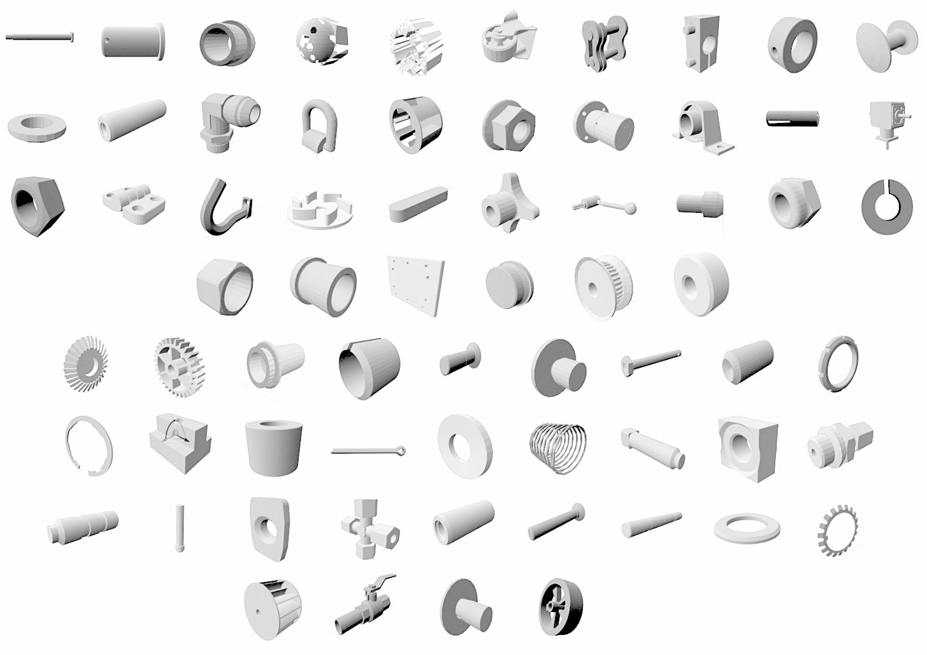
There were 67 categories of parts and 58,696 objects in total. Among them, several significant types of mechanical components existed, including nuts, pins, bearings, etc. The different types of mechanical components differed significantly, which poses a challenge to models attempting to identify them. In the following, we display the effectiveness of our model in carrying out those tasks well (see Figure 1).

3.1. Characteristics of Mechanical Components

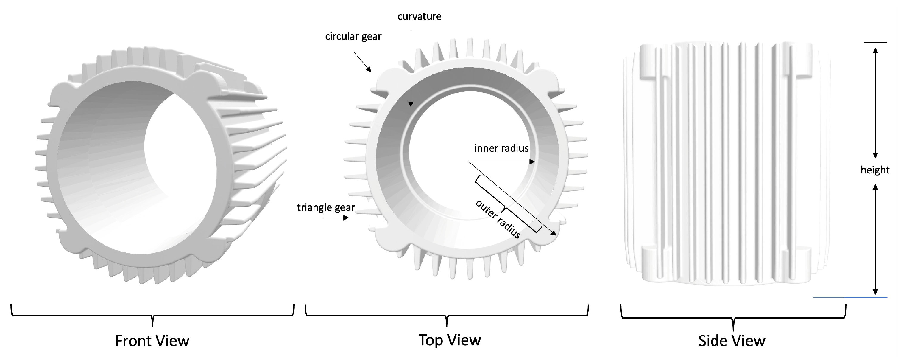
As shown in Figure 2, we estimated how many parameters a specific object had in our dataset. Notice that although the dataset had different types of mechanical components, the number of parameters should be roughly the same. We first measured the inner and outer circle radii from the motor image. In addition, we measured the height of the hollow cylinder. The circle’s edge is not completely rigid, so we added another curvature parameter. For the motor gear, we noticed different kinds of gear on the side. There were two kinds of gear on the motor: One could be approximated as part of a circle and thus had three parameters: the circle’s radius, the angle of the arc, and how much of the arc part is shown. Also, some of the gears on the circle could be modeled as a triangle. Therefore, we obtained the number of triangles, the base length, and the triangle’s height. In total, there were around ten parameters for a specific object. To use some abstract variables to capture objects’ properties, we propose using a roughly similar number of variables to describe them. The past literature on obtaining the visual features of 3D objects [33] illustrates the importance of eigenvalues in defining corners with corner detectors and on deciding other features of the object. Specifically, after observing the structure of a 3D point cloud of specific mechanical components and looking at the past literature [34,35,36,37], we decided that including linearity L, planarity P, sphericity S, omni-variance O, anisotropy A, the sum of eigenvalues $\Sigma$, and curvature C would be necessary.

We can express the values above using the eigenvalues of the neighborhood’s covariance matrix. The dimension of the covariance matrix would be $3\times 3$, so there would be three eigenvalues. We denote them by ${\lambda }_1\ge {\lambda }_2\ge {\lambda }_3>0$, as the eigenvalues of the covariance matrix are positive. Then, we have

$$\begin{array}{cc}\hfill L& ={\displaystyle \frac{{\lambda }_1-{\lambda }_2}{{\lambda }_1}}\le 1\hfill \end{array}$$

(1)

$$\begin{array}{cc}\hfill P& ={\displaystyle \frac{{\lambda }_2-{\lambda }_3}{{\lambda }_1}}\le 1\hfill \end{array}$$

(2)

$$\begin{array}{cc}\hfill S& ={\displaystyle \frac{{\lambda }_3}{{\lambda }_1}}\le 1\hfill \end{array}$$

(3)

$$\begin{array}{cc}\hfill O& =\sqrt[3]{{\lambda }_1\ast {\lambda }_2\ast {\lambda }_3}\hfill \end{array}$$

(4)

$$\begin{array}{cc}\hfill A& ={\displaystyle \frac{{\lambda }_1-{\lambda }_3}{{\lambda }_1}}\le 1\hfill \end{array}$$

(5)

$$\begin{array}{cc}\hfill \Sigma & ={\lambda }_1+{\lambda }_2+{\lambda }_3\hfill \end{array}$$

(6)

$$\begin{array}{cc}\hfill C& ={\displaystyle \frac{{\lambda }_3}{{\lambda }_1+{\lambda }_2+{\lambda }_3}}\hfill \end{array}$$

(7)

For instance, for the figure of the point cloud data of one motor above, we should depict the sphericity of the motor and the curvature of the curves.

3.2. Data Processing

We used the blender python module to process the dataset at https://pypi.org/project/bpy/ (accessed on 9 January 2025). The reason behind processing the dataset is that there will be a different number of data points in every mechanical component. To make the number of points uniform for model training without changing the structure, we should either add points to the 3D object or take a subset of the points out from the object. The latter was easier to do as we can shuffle the points and take the first 1024 points. For the first one, we used the following algorithm: we obtain the list of surfaces as triangles from the blender and then calculate the number of points we add. Suppose now we have n points in the object, and there are t triangles. Then, we add $(1024-n)/t$ points to each triangle. If t does not divide by $1024-n$, we can add more points to each triangle and sample points from the object to take points out. The main idea of our preprocessing is to ensure the object has enough points to get sent to the model while making sure that the object differs a little from the original object.

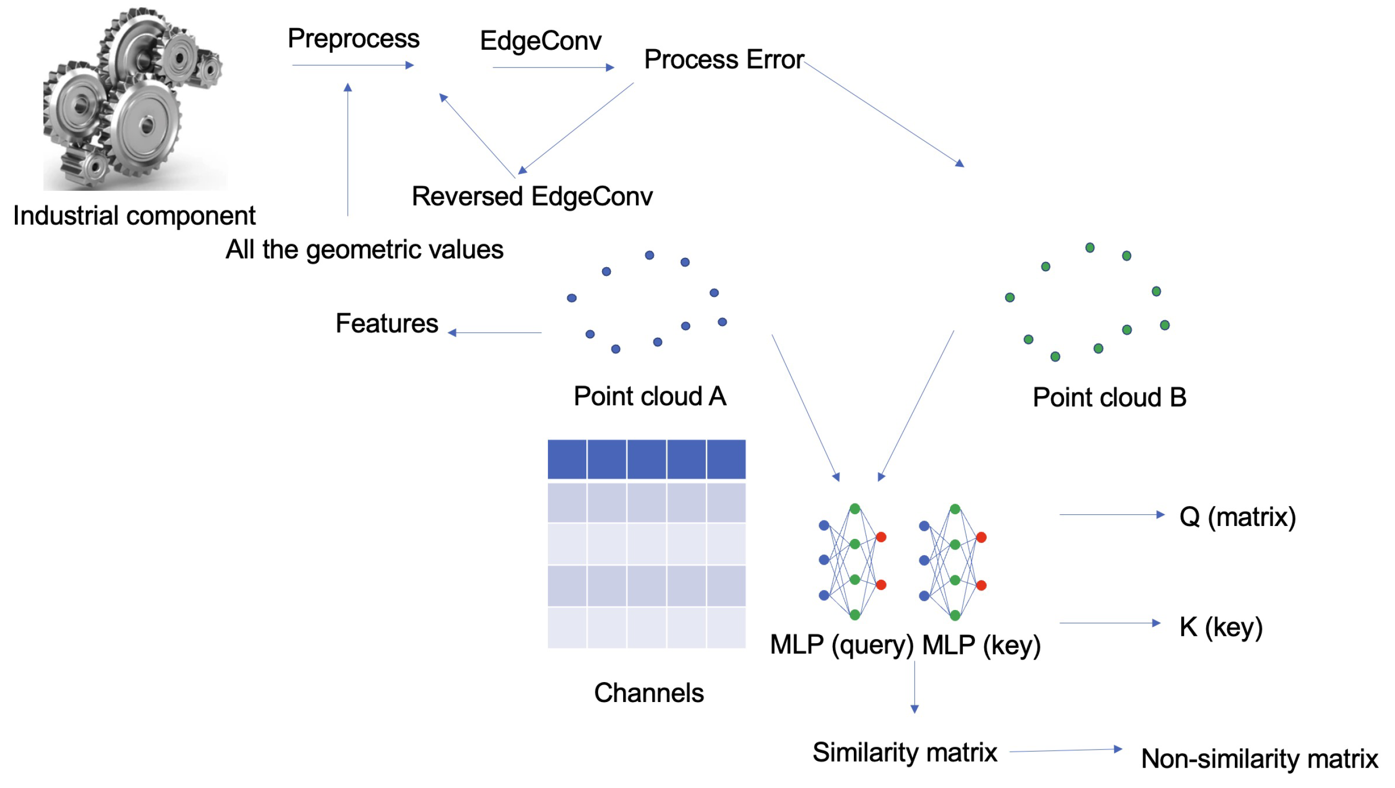
In this section, we discuss the structure of the model. We propose an approach that gives a geometric embedding to the points first and then repeatedly uses edge convolution and the attention module to obtain both fine-grained and prominent features from the point clouds.

3.3. Geometric Preprocessing

As discussed in Section 3.2, we captured the core geometric features of an object by calculating around ten variables using the covariance matrix of each neighborhood. The reason for calculating the variables only in each neighborhood was to capture the local feature of the model. There are many ways to sample the neighborhood, such as by farthest point sampling [38] in a 3D metric space using Euclidean distance with an upper bound radius r. In the neighborhood, the center is point c, the neighbor points are $p_i\in N\left(c\right)$, and we use geometric features to calculate a local pattern representation f for this neighborhood. Each point $p_i$ has its feature, and we try to process that first and then carry out aggregation:

$$f=A(F\left(f_{p_i}\right),\forall p_i)$$

(8)

where $f_{p_i}$ is the point feature $p_i$. In this paper, $p_i$ denotes the 3D coordinates of point $p_i$ expressed as a vector.

We concatenate all the variables into a vector $G_v$, which is

$$G_v=[L,P,S,A,\Sigma ,C,O]$$

(9)

In the equation above, all elements such as $L,P,$ and $\Sigma$, are the ones that are defined in Section 3.1.

After calculating the geometric features, we concatenate the feature vector with the original vector, which results in the following (after normalization):

$$F\left(f_{p_i}\right)=[\mathrm{MLP}\left(G_v\right),f_{p_i}]$$

(10)

3.4. Attention for Point Clouds

In this section, we introduce how to calculate attention on point clouds. We will first demonstrate how we calculate the attention between two point clouds using two parts: calculating a similarity matrix between the point clouds and then converting the similarity matrix into an affinity matrix.

To calculate the similarity matrix, we first need to reduce the computation space using a shared MLP to operate a channel vector $c_i\in R^S$ (S represents the original number of points) to reduce the point cloud tensors into tensors of smaller sizes. Specifically, we use two MLPs, $N_{query}$ and $N_{keys}$, to obtain the query matrix and key matrix to calculate attention. The query matrix and key matrix would look like the following:

$$Q=[q_1,q_2,\dots ,q_n]\in R^{S^{\prime }\times n}K=[k_1,k_2,\dots ,k_n]\in R^{S^{\prime }\times n}$$

(11)

where $S^{\prime }$ is the reduced dimension from S, and n is the dimension of the feature map, as seen in Figure 3. Then, we can estimate the similarity matrix $M_s$ (channel-wise) to be

$$M_s=Q^{⊺}K$$

(12)

where the ith row and jth column matrix would be the similarity between the ith channel and jth channel of the given feature map.

After deriving the similarity matrix, we use it to calculate the long-range dependencies following a self-attention structure, which requires taking inner products with the value matrix and our similarity matrix. We choose to process our channel-wise similarity matrix $M_s$ into a matrix that describes non-similarity, according to the following equation:

$$N_s=\mathrm{expand}\mathrm{dimension}(max\left(M_s\right))-M_s$$

(13)

In the equation above, we select the maximum similarities along each column of $M_s$ and expand them so the channels in $M_s$ that have higher similarities would have lower values. Then, we apply soft-max on matrix $N_s$ for normalization. We take a weighted sum of all the channels by multiplying that with our value matrix to obtain a refined feature map.

3.5. Graph Neural Network

Considering the properties of the points in the point cloud, we treat the whole point cloud as a graph neural network (GNN). To set up the network, we first compute a directed graph $G=(V,E)$, representing the cloud structure. There are many ways to compute the graph based on the given vertices, including the most basic way of computing a k-nearest neighbor (k-NN) graph, where k is a hyperparameter to be tuned for the vertices. In each neighborhood, we connect pairs of vertices inside it. Therefore, a vertex will be connected to itself, and such self-loops in the graph are fine. We denote the set of vertices as V and edges as $E\subseteq V\times V$.

Now, we define the edge feature for this graph, as it defines the important relationship between points in the point cloud. For two points $p_i$ and $p_j$ in the point cloud, we use a nonlinear function with learnable parameters, f, to obtain the edge feature. In other words, the edge feature $e_{ij}$ between points $p_i$ and $p_j$ is equal to

$$e_{ij}=f(p_i,p_j).$$

Then, we define edge convolution, which aggregates the edge features with all edges from a vertex. The equation just applies an aggregation function on it, i.e., the feature $x_i$ for point i is

$$x_i^{\prime }=g_{j:(i,j)\in E}f(p_i,p_j)$$

There are several choices for g and f. However, considering that we want to keep the function simple while capturing the global and local information of the point cloud, we use the point’s value, $p_i$, to express the global information. For local information, on the other hand, we use the difference between the points’ values, $p_i-p_j$, to express the local information. Adding in the aggregation function, we have the edge convolution of the form

$$x_i{m}^{\prime }=\underset{j:(i,j)\in E}{max}\mathrm{ReLU}({\theta }_{1_m}·(p_j-p_i)+{\theta }_{2_m}·x_i)$$

3.6. Reverse the Edge Convolution

As we use edge convolution to process the point clouds to retrieve its geometric features, we can restore the edge convolution result back to its input, which is like the result of reversing edge convolution, inspired by the auto-encoder approach. We use a shared fully connected layer, $L_r$ to reverse the input processed by the edge convolution layer, $L_e$. Then, we take the difference between the original and reversed inputs to formulate the error:

$$\delta x_i=L_r\left(L_e\left(x_i\right)\right)-x_i$$

(14)

The calculation of the error is inspired by the design of auto-encoders, although here we only change the size of the feature instead of the size of the point clouds.

Then, we use max pooling to extract the prominent features, and append those prominent features to the ones obtained by applying edge convolution to the point cloud. Finally, we use the attention module we described in Section 3.4 to process the result and obtain the features that are important.

3.7. Fine-Grained Geometric Features

However, for more complex shapes in the mechanical components, we would need to obtain the fine-grained geometric features, and we first apply edge convolution to the point clouds, then a fully connected layer, and then, finally, our attention module. In the end, we have two features, one representing the global prominent features of the point cloud, and one for fine-grained features of the point cloud. We finally concatenate them and obtained our learned geometric features.

3.8. Proof of Invariance

We also prove that the function we found before can process point clouds, which means that the function we picked before to process the data at each layer satisfies Permutation Invariance and Translation Invariance. For further details, please refer to Appendix A.

4. Experiments and Results

This section evaluates the model’s performance and discusses the result on the basis of the dataset of mechanical components. To show the potential of the model, we assess the model from several aspects. First, we chose several evaluation metrics to show the model’s accuracy. The metrics include a confusion matrix, ROC curve, and so on, showing that our model has a solid true positive rate and a solid true negative rate. Other than that, we also compare our model with one of the state-of-the-art models; dynamic graph CNN (DGCNN) and our model display a strong advantage in classification. Overall, the following sections show how strong our model is.

4.1. Evaluation Metrics

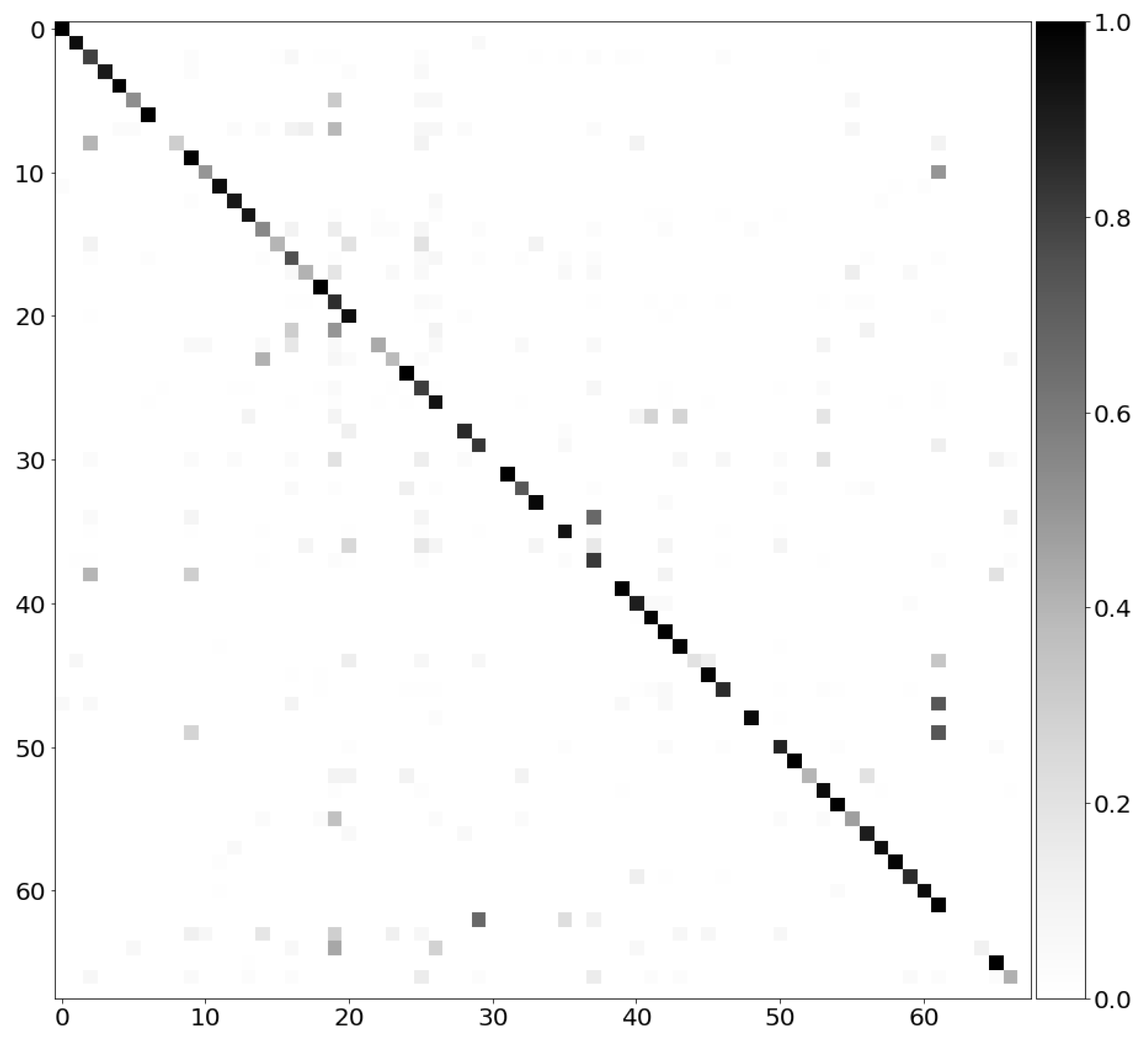
We first discuss the confusion matrix and our model’s performance. The confusion matrix shows how well our model performs in supervised learning, specifically in classifying the geometrical objects; in this case, inside the confusion matrix, the number of columns (or rows) matches the number of types for classification. Each row of the matrix represents an instance of an actual class, while each column represents an instance of the predicted class. The darker the color in a grid, the more instances there are. The ideal performance of a model would be that the diagonal of the matrix would be very dark, meaning there are fewer false positive and false negative samples.

To generate the confusion matrix on our dataset, we calculated the prediction on each label and normalized it by dividing the prediction by the total number of predictions. The confusion matrix looks like the one below in gray-scale.

As seen in the confusion matrix diagram above Figure 4, there is a pattern consisting of self-explanatory dark-colored blocks on the diagonal, which means the model achieves a high true positive rate for most types. The color of blocks for other regions in the matrix is not as dark as the ones on the diagonal, which means our model also achieves a low false positive/false negative rate on most labels.

4.2. Comparison to Baseline Models

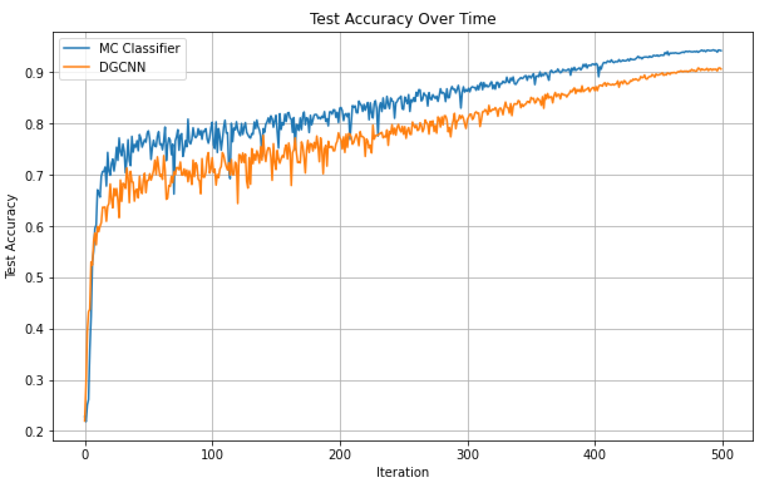
In this section, we discuss how our method compares to DGCNN, which is the backbone of our model, to show how much our geometric-centric aware module and attention module help in classifying objects.

In Figure 5, we can see that our model achieves a higher accuracy than DGCNN. As we can see, our model reaches a higher accuracy within a reasonable number of epochs.

After showing the extensive evaluation figures and detailed comparison between our model and the DGCNN, we can see that our model performs well by itself, reaching low false negative and false positive rates, and can perform well under any threshold. In addition, compared to other SOTA architecture, our model displays its advantage by incorporating geometric preprocessing: it is more resistant to overfitting and can reach a higher accuracy in the long run by capturing local geometric information.

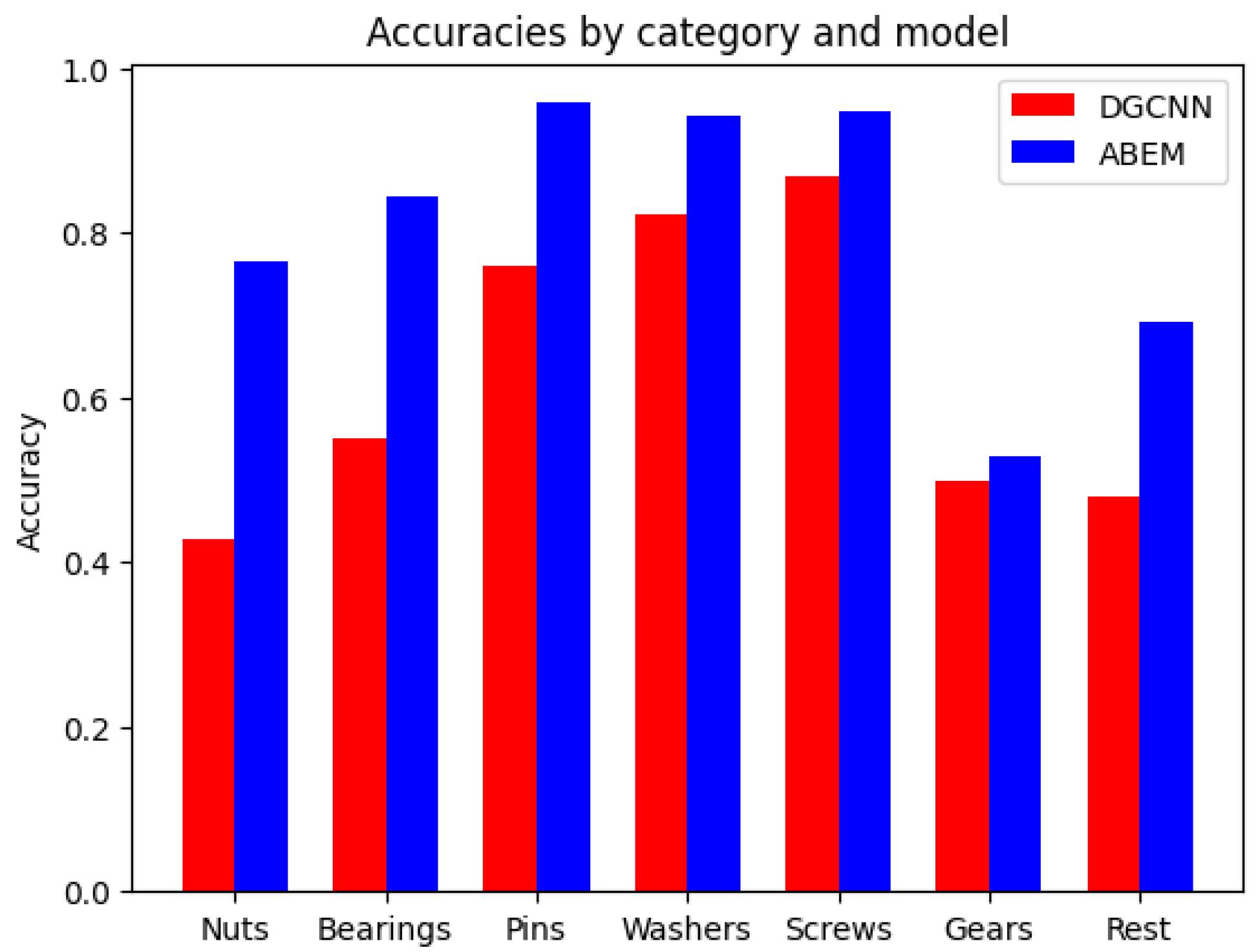
4.3. Comparison on Different Subcategories of Mechanical Components

In this section, we compare the accuracy of our model to DGCNN on different categories of components. We divided the mechanical components into the following categories: 1—nuts; 2—bearings; 3—pins; 4—washers; 5—screws; and 6—gear. We compared our model’s performance to the DGCNN’s performance, as shown in the table below as well as in the visualization.

As shown in Figure 6 and

Table 1. Comparison of accuracies.

Component Category	DGCNN	MC Classifier
Nuts	0.426	0.764
Bearings	0.549	0.844
Pins	0.760	0.958
Washers	0.822	0.943
Screws	0.870	0.947
Gears	0.499	0.530
Rest	0.478	0.691

, our model behaves better than the DGCNN in every category, showing the effectiveness of the attention and geometric-aware module in classifying those objects.

5. Conclusions

To address the increasing need for classifying mechanical components in pipelines, we propose a state-of-the-art model that effectively identifies mechanical components that are incredibly complicated due to their intriguing details among other visual objects. The model achieves outstanding performance through its use of geometric priori, emphasizing the importance of the local structure of the objects. The geometric variables can describe a mechanical component from scratch in detail. In addition, we scaled the model so that it can capture the global structure of an object by propagating it through a modern graph neural network structure. The model achieves excellent performance. Compared to other state-of-the-art models, the model can achieve better results.

The model would help to streamline pipelines in mechanical production. Once the point cloud of all mechanical components is available, the new model can be trained with moderate computation within a day, and when classifying objects in the pipeline, no additional task is needed other than inference, which takes seconds. To incorporate the MC-Classifier system in real-world applications, the practitioner should obtain point cloud models for all the mechanical components in production and build a dataset of them; this is the only thing needed to train the framework. During inference, the practitioner should load the components into a point cloud framework for analysis so that the inference works. Other than just classifying, the framework of MC Classifier can also be potentially applied to other areas of the pipeline, such as identifying defects in the components or the efficient maintenance of the pipeline logistics by counting the number of each industrial component.

On the other hand, the model presented in this paper should inspire more geometry-based computer vision models. For tasks that involve dealing with objects with detailed local structures, other than stacking neural network structures, one could approach them by considering the incorporation of geometric variables into the whole neural network model. As presented in this paper, such considerations regarding the objects’ geometric properties could result in models with better performance than models without such considerations. For now, factories could use the proposed model in the industry to automate tasks when producing such components. On the other hand, the tremendous potential that this paper offers is that similar geometry methods could be applied to different datasets involving delicate objects such as plants, components for automobiles, and so on, and using geometry before boosting a neural network’s performance would be worth studying further.

6. Future Work

In this work, we delivered a novel framework, MC Classifier, that can effectively identify mechanical components and outperform the current state-of-the-art models in determining the type of mechanical components. However, there is still room for improvement in this model and further exploration to carry out with the framework. For instance, alternative approaches, such as capturing the essential quantities of the mechanical elements into a bottleneck, might result in different performances. Also, the network structure could be tuned further to ensure better performance. In addition, there is still more to explore regarding the model’s effectiveness on other types of 3D objects and in testing MC Classifier in real production environments. Potential challenges in integrating the model into industrial systems might include converting real-life components into point cloud data efficiently.

References

- Ng, W.L.; Goh, G.L.; Goh, G.D.; Ten, J.S.J.; Yeong, W.Y. Progress and opportunities for machine learning in materials and processes of additive manufacturing. Adv. Mater. 2024, 36, 2310006. [Google Scholar] [CrossRef] [PubMed]
- Shahin, M.; Chen, F.F.; Hosseinzadeh, A.; Zand, N. Using machine learning and deep learning algorithms for downtime minimization in manufacturing systems: An early failure detection diagnostic service. Int. J. Adv. Manuf. Technol. 2023, 128, 3857–3883. [Google Scholar] [CrossRef]
- Saeed, A.; Khan, M.A.; Akram, U.; Obidallah, W.J.; Jawed, S.; Ahmad, A. Deep learning based approaches for intelligent industrial machinery health management and fault diagnosis in resource-constrained environments. Sci. Rep. 2025, 15, 1114. [Google Scholar] [CrossRef] [PubMed]
- Jia, Z.; Wang, M.; Zhao, S. A review of deep learning-based approaches for defect detection in smart manufacturing. J. Opt. 2024, 53, 1345–1351. [Google Scholar] [CrossRef]
- Archana, R.; Jeevaraj, P.E. Deep learning models for digital image processing: A review. Artif. Intell. Rev. 2024, 57, 11. [Google Scholar] [CrossRef]
- Nie, Z.; Lin, T.; Jiang, H.; Kara, L.B. Topologygan: Topology optimization using generative adversarial networks based on physical fields over the initial domain. J. Mech. Des. 2021, 143, 031715. [Google Scholar] [CrossRef]
- Cynthia, E.P.; Ismanto, E.; Arifandy, M.I.; Sarbaini, S.; Nazaruddin, N.; Manuhutu, M.A.; Akbar, M.A.; Abdiyanto. Convolutional Neural Network and Deep Learning Approach for Image Detection and Identification. Proc. J. Phys. Conf. Ser. 2022, 2394, 012019. [Google Scholar] [CrossRef]
- Li, Z.; Liu, F.; Yang, W.; Peng, S.; Zhou, J. A survey of convolutional neural networks: Analysis, applications, and prospects. IEEE Trans. Neural Netw. Learn. Syst. 2021, 33, 6999–7019. [Google Scholar] [CrossRef] [PubMed]
- Su, H.; Maji, S.; Kalogerakis, E.; Learned-Miller, E. Multi-view convolutional neural networks for 3d shape recognition. In Proceedings of the IEEE International Conference on Computer Vision, Santiago, Chile, 7–13 December 2015; pp. 945–953. [Google Scholar]
- Hong, Y.; Lin, C.; Du, Y.; Chen, Z.; Tenenbaum, J.B.; Gan, C. 3d concept learning and reasoning from multi-view images. In Proceedings of the IEEE/CVF Conference on Computer Vision and Pattern Recognition, Vancouver, BC, Canada, 17–24 June 2023; pp. 9202–9212. [Google Scholar]
- Feng, Y.; Zhang, Z.; Zhao, X.; Ji, R.; Gao, Y. GVCNN: Group-view convolutional neural networks for 3D shape recognition. In Proceedings of the IEEE Conference on Computer Vision and Pattern Recognition, Salt Lake City, UT, USA, 18–23 June 2018; pp. 264–272. [Google Scholar]
- Zhu, Z.; Wang, X.; Bai, S.; Yao, C.; Bai, X. Deep learning representation using autoencoder for 3D shape retrieval. Neurocomputing 2016, 204, 41–50. [Google Scholar] [CrossRef]
- Nie, Z.; Lynn, R.; Tucker, T.; Kurfess, T. Voxel-based analysis and modeling of MRR computational accuracy in milling process. CIRP J. Manuf. Sci. Technol. 2019, 27, 78–92. [Google Scholar] [CrossRef]
- Maturana, D.; Scherer, S. Voxnet: A 3d convolutional neural network for real-time object recognition. In Proceedings of the 2015 IEEE/RSJ International Conference on Intelligent Robots and Systems (IROS), Hamburg, Germany, 28 September–2 October 2015; pp. 922–928. [Google Scholar]
- Riegler, G.; Osman Ulusoy, A.; Geiger, A. Octnet: Learning deep 3d representations at high resolutions. In Proceedings of the IEEE Conference on Computer Vision and Pattern Recognition, Las Vegas, NV, USA, 27–30 June 2016; pp. 3577–3586. [Google Scholar]
- Klokov, R.; Lempitsky, V. Escape from cells: Deep kd-networks for the recognition of 3d point cloud models. In Proceedings of the IEEE International Conference on Computer Vision, Venice, Italy, 22–29 October 2017; pp. 863–872. [Google Scholar]
- Zeng, W.; Gevers, T. 3dcontextnet: Kd tree guided hierarchical learning of point clouds using local and global contextual cues. In Proceedings of the European Conference on Computer Vision (ECCV) Workshops, Munich, Germany, 8–14 September 2018. [Google Scholar]
- Xu, C.; Bai, Y.; Bian, J.; Gao, B.; Wang, G.; Liu, X.; Liu, T.Y. Rc-net: A general framework for incorporating knowledge into word representations. In Proceedings of the 23rd ACM International Conference on Conference on Information and Knowledge Management, Shanghai, China, 3–7 November 2014; pp. 1219–1228. [Google Scholar]
- Li, J.; Chen, B.M.; Lee, G.H. So-net: Self-organizing network for point cloud analysis. In Proceedings of the IEEE Conference on Computer Vision and Pattern Recognition, Salt Lake City, UT, USA, 18–23 June 2018; pp. 9397–9406. [Google Scholar]
- Qi, C.R.; Su, H.; Mo, K.; Guibas, L.J. Pointnet: Deep learning on point sets for 3d classification and segmentation. In Proceedings of the IEEE Conference on Computer Vision and Pattern Recognition, Las Vegas, NV, USA, 27–30 June 2016; pp. 652–660. [Google Scholar]
- Qi, C.R.; Yi, L.; Su, H.; Guibas, L.J. Pointnet++: Deep hierarchical feature learning on point sets in a metric space. In Proceedings of the Advances in Neural Information Processing Systems, Long Beach, NY, USA, 4–9 December 2017; Volume 30. [Google Scholar]
- Vaswani, A.; Shazeer, N.; Parmar, N.; Uszkoreit, J.; Jones, L.; Gomez, A.N.; Kaiser, Ł.; Polosukhin, I. Attention is all you need. In Proceedings of the Advances in Neural Information Processing Systems, Long Beach, NY, USA, 4–9 December 2017; Volume 30. [Google Scholar]
- Hu, J.; Shen, L.; Sun, G. Squeeze-and-excitation networks. In Proceedings of the IEEE Conference on Computer Vision and Pattern Recognition, Salt Lake City, UT, USA, 18–23 June 2018; pp. 7132–7141. [Google Scholar]
- Xie, S.; Liu, S.; Chen, Z.; Tu, Z. Attentional shapecontextnet for point cloud recognition. In Proceedings of the IEEE Conference on Computer Vision and Pattern Recognition, Salt Lake City, UT, USA, 18–23 June 2018; pp. 4606–4615. [Google Scholar]
- Feng, M.; Zhang, L.; Lin, X.; Gilani, S.Z.; Mian, A. Point attention network for semantic segmentation of 3D point clouds. Pattern Recognit. 2020, 107, 107446. [Google Scholar] [CrossRef]
- Veličković, P.; Cucurull, G.; Casanova, A.; Romero, A.; Lio, P.; Bengio, Y. Graph attention networks. arXiv 2017, arXiv:1710.10903. [Google Scholar]
- Simonovsky, M.; Komodakis, N. Dynamic edge-conditioned filters in convolutional neural networks on graphs. In Proceedings of the IEEE Conference on Computer Vision and Pattern Recognition, Honolulu, HI, USA, 21–26 July 2017; pp. 3693–3702. [Google Scholar]
- Wang, Y.; Sun, Y.; Liu, Z.; Sarma, S.E.; Bronstein, M.M.; Solomon, J.M. Dynamic graph cnn for learning on point clouds. ACM Trans. Graph. (tog) 2019, 38, 1–12. [Google Scholar] [CrossRef]
- Hassani, K.; Haley, M. Unsupervised multi-task feature learning on point clouds. In Proceedings of the IEEE/CVF International Conference on Computer Vision, Seoul, Republic of Korea, 27 October–2 November 2019; pp. 8160–8171. [Google Scholar]
- Chen, C.; Li, G.; Xu, R.; Chen, T.; Wang, M.; Lin, L. Clusternet: Deep hierarchical cluster network with rigorously rotation-invariant representation for point cloud analysis. In Proceedings of the IEEE/CVF Conference on Computer Vision and Pattern Recognition, Long Beach, CA, USA, 15–20 June 2019; pp. 4994–5002. [Google Scholar]
- Nie, Z.; Jiang, H.; Kara, L.B. Stress field prediction in cantilevered structures using convolutional neural networks. J. Comput. Inf. Sci. Eng. 2020, 20, 011002. [Google Scholar] [CrossRef]
- Kim, S.; Chi, H.g.; Hu, X.; Huang, Q.; Ramani, K. A Large-scale Annotated Mechanical Components Benchmark for Classification and Retrieval Tasks with Deep Neural Networks. In Proceedings of the 16th European Conference on Computer Vision (ECCV), Glasgow, UK, 23–28 August 2020. [Google Scholar]
- Weinmann, M. Visual features—From early concepts to modern computer vision. In Advanced Topics in Computer Vision; Springer: London, UK, 2013; pp. 1–34. [Google Scholar]
- Li, J.; Zhao, J.; Kang, Y.; He, X.; Ye, C.; Sun, L. Dl-slam: Direct 2.5 d lidar slam for autonomous driving. In Proceedings of the 2019 IEEE Intelligent Vehicles Symposium (IV), Paris, France, 9–12 June 2019; pp. 1205–1210. [Google Scholar]
- Huang, K.; Dong, Z.; Wang, J.; Fei, Y. Weld bead segmentation using RealSense depth camera based on 3D global features and texture features of subregions. Signal Image Video Process. 2023, 17, 2369–2383. [Google Scholar] [CrossRef]
- Weinmann, M. Feature relevance assessment for the semantic interpretation of 3D point cloud data. ISPRS Ann. Photogramm. 2013, 2, 313–318. [Google Scholar] [CrossRef]
- Li, W.; Wang, F.D.; Xia, G.S. A geometry-attentional network for ALS point cloud classification. ISPRS J. Photogramm. Remote Sens. 2020, 164, 26–40. [Google Scholar] [CrossRef]
- Moenning, C.; Dodgson, N.A. Fast Marching Farthest Point Sampling; Technical Report UCAM-CL-TR-562; University of Cambridge, Computer Laboratory: Cambridge, UK, 2003. [Google Scholar] [CrossRef]