Research on Concentricity Detection Method of Automobile Brake Piston Parts Based on Improved Canny Algorithm

Abstract

The automotive brake piston component is an important part of the automotive brake system, and the concentricity detection of the first piston component is crucial to ensure driving safety. In this paper, an improved Canny algorithm is proposed for non-contact detection of spring concentricity of the first piston component. Firstly, the traditional Canny algorithm is improved by replacing the Gaussian filter with a bilateral filter to fully retain the edge information, and accurate edge detection results are obtained by constructing a multi-scale analysis. After obtaining the edge images, a sub-pixel edge detection method with gray moments is introduced to optimize these edges; secondly, a circle is fitted to the extracted edge points by using the RANSAC algorithm to determine the center position and radius of the circle; and finally, the concentricity of the first piston part is calculated based on the fitting results. The experimental results are compared with those of the CMM and the traditional Canny algorithm, and the results show that the improved Canny algorithm reduces the coaxiality error by 4% and enables effective measurement of the concentricity of the first piston assembly spring.

1. Introduction

In the field of mechanical processing, concentricity is an important technical indicator for evaluating the alignment accuracy of cylindrical workpieces. The quality of concentricity directly affects the assembly quality, performance, operational stability, and lifespan of the entire mechanical system. The most crucial step in concentricity detection is circle fitting, and scholars at home and abroad have conducted extensive research on circle fitting algorithms. Zhehong Guo from Nanchang University proposed an edge point screening method [1] and combined sub-pixel edge detection with circle center positioning. This algorithm has high detection accuracy and anti-noise ability. Lei Zhu et al. achieved real-time measurement and adjustment of the coaxiality of parts by improving methods such as one-dimensional measurement of rectangles to find boundary points [2]. This method has the characteristics of high speed, high robustness, and high precision. Jiawen Wang et al. proposed an image edge detection method using sinusoidal moving fitting [3], which has the characteristics of high measurement accuracy and good stability compared to the traditional random Hough transform. Yongzhi Peng et al. proposed a multi-bottle mouth positioning algorithm based on DBSCAN random circle detection [4], which has high accuracy and real-time performance. Chengli Zhao et al. proposed an optimization method for circle center fitting based on photogrammetry and Hough transform [5], which effectively solved the problem of the inability to directly measure the circle center on construction machinery. Jianfeng Guo et al. proposed an iterative method for robust circle fitting [6], and the proposed iterative procedure can reduce the impact of abnormal values on the estimation of circle parameters. Maja Michałowska et al. combined Hough transform, the de-noising process, and the robust least squares circle fitting method [7] to extract the position of tree stem segments from terrestrial laser scanning data. Yun Ou et al. proposed a fast circle detection algorithm based on information compression [8]. Xianen Zhou et al. proposed a new circle detection MFLS algorithm based on model fitting and the least squares technique [9], which has strong anti-interference ability. Shuyi Guo et al. addressed the issue of circular projections becoming elliptical in optical CCD detection and proposed a circle detection algorithm based on ellipse de-noising [10]. At present, modern methods based on image processing, laser measurement, and three-coordinate detection have become research hotspots, but they have certain limitations. For example, algorithms based on Canny edge detection and Hough transform are susceptible to noise interference and require a large amount of computation. Laser measuring instruments [11] have high precision but expensive costs and poor environmental adaptability. Although the coordinate measuring machine (CMM) [12] has excellent accuracy, it has low detection efficiency and complex operation. The existing concentricity detection of piston components mostly adopts manual eye inspection, which has low efficiency and large subjective error. Therefore, how to optimize existing methods or explore new detection techniques to achieve high precision, high efficiency, and low-cost concentricity measurement is still an urgent problem to be solved.

Aiming at the problems of low efficiency and large subjective error of manual eye inspection in concentricity detection of piston components, this study proposes an improved Canny algorithm for non-contact detection of the concentricity of the spring in the first piston component. The improved Canny algorithm can effectively suppress false edges and retain more edge information, and, at the same time, the improved Canny algorithm reduces the concentricity error by 4%, resulting in an effective non-contact measurement of the spring concentricity of the first piston component.

2. Traditional Canny Algorithm and Its Improvement

2.1. Traditional Canny Algorithm

2.1.1. Algorithm Principle

The Canny algorithm is a classical edge detection algorithm [13], the core idea of which is to accurately locate the edge of the image through multi-stage processing, while suppressing noise. The algorithm consists of the following four steps:

(1)

Gaussian filtering: Firstly, the original image is smoothed by Gaussian to eliminate high-frequency noise and avoid interference in subsequent gradient calculation.

(2)

Gradient calculation and direction extraction: The Sobel operator (two small matrices) is used to calculate the gradient of the image in the horizontal (x) and vertical (y) directions, respectively. Based on the gradients in the x and y directions, calculate the gradient intensity (how sharp the edge is) and the direction (whether the edge is facing left/right/up/down) for each pixel. The gradient amplitude reflects the edge strength, and the direction indicates the potential direction of the edge.

(3)

Non-maximum suppression: The amplitude is locally compared in the gradient direction, only the pixels with the largest amplitude are retained, and the edge width is refined to the single pixel level to eliminate redundant responses.

(4)

Double threshold detection and edge connection: Candidate edges are screened by high and low thresholds: strong edges are determined by high thresholds, weak edges are retained by low thresholds, and weak edges are connected to strong edges in combination with connectivity analysis to ensure the continuity and integrity of edges.

2.1.2. Limitations

The advantage of the traditional Canny algorithm is that it can balance noise suppression and edge location accuracy, but there are some difficult problems to solve. The oversmoothing problem of the Gaussian filter: the standard Gaussian filter will blur the step edge while reducing noise, resulting in the loss of weak edge; limitations of fixed thresholds: global thresholds can produce broken edges when illumination is uneven; and pixel level accuracy is insufficient: the error of traditional methods in sub-micron level measurement tasks can reach 5–8% [14].

2.2. Improved Canny Algorithm

The traditional Canny algorithm uses Gaussian filtering for preprocessing in the filtering and noise removal part, and in the process of removing noise, it will overly clean the edge information of the image, Some edge information may be lost. In this regard, this paper replaces the Gaussian filter with a bilateral filter for image preprocessing to retain more edge information. The Sobel operator in the Canny algorithm usually performs edge detection at a single scale, which will lead to the loss of some details and affect the edge detection accuracy. To solve this problem, this paper adopts multi-scale analysis, detects edges at different scales by constructing an image pyramid, and then fuses the results to obtain more comprehensive and accurate edge information. To further improve the edge detection accuracy, this paper introduces the sub-pixel edge detection method based on the gray moment in the Canny algorithm, upgrading the Canny algorithm from full-pixel accuracy to sub-pixel accuracy, providing a guarantee for the accuracy of subsequent circle fitting and concentricity calculation.

2.2.1. Bilateral Filtering

Bilateral filtering is a non-linear filtering method [15]. It combines the information of spatial neighborhood and gray value similarity and can retain edge information while removing noise. This method is particularly suitable for noise reduction scenarios where edges need to be retained. The bilateral filter is composed of two Gaussian filters. One is used to calculate the weight of the spatial proximity of the image, and the other is used to calculate the weight of the similarity of the image pixel values [16]. The expression of the bilateral filter is shown in Equation (1).

$$\mathrm{B}\left(\mathrm{i},\mathrm{j},\mathrm{k},\mathrm{l}\right)=\exp \left(-{\displaystyle \frac{{\left(\mathrm{i}-\mathrm{k}\right)}^2+{\left(\mathrm{j}-\mathrm{l}\right)}^2}{2{\mathsf{\sigma }}_{\mathrm{s}}^2}}\right)\times \exp \left(-{\displaystyle \frac{{\left|\mathrm{M}\left(\mathrm{i},\mathrm{j}\right)-\mathrm{M}\left(\mathrm{k},\mathrm{l}\right)\right|}^2}{2{\mathsf{\sigma }}_{\mathrm{r}}^2}}\right)$$

(1)

In the equation, $\left(\mathrm{i},\mathrm{j}\right)$ and $\left(\mathrm{k},\mathrm{l}\right)$ denote the coordinates of the center pixel and neighboring pixels, respectively; $\mathrm{M}\left(\mathrm{i},\mathrm{j}\right)$ and $\mathrm{M}\left(\mathrm{k},\mathrm{l}\right)$ denote their pixel values, respectively; ${\mathsf{\sigma }}_{\mathrm{s}}$ and ${\mathsf{\sigma }}_{\mathrm{r}}$ are the standard deviations of the null and value domains, respectively; and exp represents the exponential function with the natural logarithm e as the base.

2.2.2. Multi-Scale Analysis

Edges in an image may exist at different scales. Small scales can detect detailed edges in the image, but are more sensitive to noise; large scales can detect the main edge structures in the image, and are relatively less sensitive to noise, but may lose some details. The purpose of multi-scale analysis is to integrate edge information at different scales to obtain more comprehensive and accurate edge detection results. The image pyramid is a very intuitive multi-scale representation structure, and multi-scale analysis is obtained by analyzing a series of images with different resolutions.

By constructing an image pyramid, images with different resolutions (scales) can be obtained. The Sobel operator is applied to these images at different scales for edge detection, and then the results of these edge detections are fused so that while retaining edge details, the main edge structures can also be obtained.

For the original image ${\mathrm{I}}_0\left(\mathrm{x},\mathrm{y}\right)$, an image pyramid is constructed. The calculation method of the k-th layer image ${\mathrm{I}}_{\mathrm{k}}\left(\mathrm{x},\mathrm{y}\right)$ is shown in Equation (2).

$${\mathrm{I}}_{\mathrm{k}}\left(\mathrm{x},\mathrm{y}\right)={\mathrm{I}}_{\mathrm{k}-1}^{\prime }\left(\mathrm{x},\mathrm{y}\right)={\mathrm{I}}_{\mathrm{k}-1}\left(\mathrm{x},\mathrm{y}\right)\ast \mathrm{B}\left(\mathrm{i},\mathrm{j},\mathrm{k},\mathrm{l}\right)$$

(2)

In the equation, ${\mathrm{I}}_{\mathrm{k}-1}^{\prime }\left(\mathrm{x},\mathrm{y}\right)$ denotes the bilateral filtering of ${\mathrm{I}}_{\mathrm{k}-1}\left(\mathrm{x},\mathrm{y}\right)$, $\ast$ denotes the convolution operation, and $\mathrm{B}\left(\mathrm{i},\mathrm{j},\mathrm{k},\mathrm{l}\right)$ is the bilateral filtering function.

Downsampling is then performed to obtain ${\mathrm{I}}_{\mathrm{k}}\left(\mathrm{x},\mathrm{y}\right)$. Downsampling usually involves reducing the rows and columns of the image by a certain percentage, taking one pixel point per row and column. In general, as k increases, the scale of the image becomes smaller.

For each layer of the image ${\mathrm{I}}_{\mathrm{k}}\left(\mathrm{x},\mathrm{y}\right)$ in the pyramid, the Sobel operator is applied to compute the gradient magnitude and direction. The Sobel operator has a horizontal template ${\mathrm{G}}_{\mathrm{x}}=\left[\begin{array}{ccc}-1& 0& 1\\ -2& 0& 2\\ -1& 0& 1\end{array}\right]$ and a vertical template ${\mathrm{G}}_{\mathrm{y}}=\left[\begin{array}{ccc}-1& -2& -1\\ 0& 0& 0\\ 1& 2& 1\end{array}\right]$.

For image ${\mathrm{I}}_{\mathrm{k}}\left(\mathrm{x},\mathrm{y}\right)$, calculate the horizontal gradient ${\mathrm{G}}_{\mathrm{x},\mathrm{k}}={\mathrm{I}}_{\mathrm{k}}\left(\mathrm{x},\mathrm{y}\right){ \ast \mathrm{G}}_{\mathrm{x}}$, the vertical gradient ${\mathrm{G}}_{\mathrm{y},\mathrm{k}}={\mathrm{I}}_{\mathrm{k}}\left(\mathrm{x},\mathrm{y}\right){ \ast \mathrm{G}}_{\mathrm{y}}$ (here $\ast$ also indicates convolution operation), the gradient magnitude ${\mathrm{G}}_{\mathrm{k}}\left(\mathrm{x},\mathrm{y}\right)=\sqrt{{\mathrm{G}}_{\mathrm{x},\mathrm{k}}^2+{\mathrm{G}}_{\mathrm{y},\mathrm{k}}^2}$, and the gradient direction ${\mathsf{\theta }}_{\mathrm{k}}=\arctan \left({\displaystyle \frac{{\mathrm{G}}_{\mathrm{y},\mathrm{k}}}{{\mathrm{G}}_{\mathrm{x},\mathrm{k}}}}\right)$.

The gradient magnitudes obtained at different scales are weighted and summed. Set ${\mathrm{G}}_{\mathrm{final}}\left(\mathrm{x},\mathrm{y}\right)={\sum }_{\mathrm{k}=0}^{\mathrm{N}-1}{\mathsf{\omega }}_{\mathrm{k}}{\mathrm{G}}_{\mathrm{k}}\left(\mathrm{x},\mathrm{y}\right)$, where $\mathrm{N}$ is the number of layers of the image pyramid and ${\mathsf{\omega }}_{\mathrm{k}}$ is the weight of the k-th layer, so that images at larger scales (lower layers) are weighted more heavily to emphasize major edge structures, while images at smaller scales (higher layers) are weighted less heavily to preserve detailed edges.

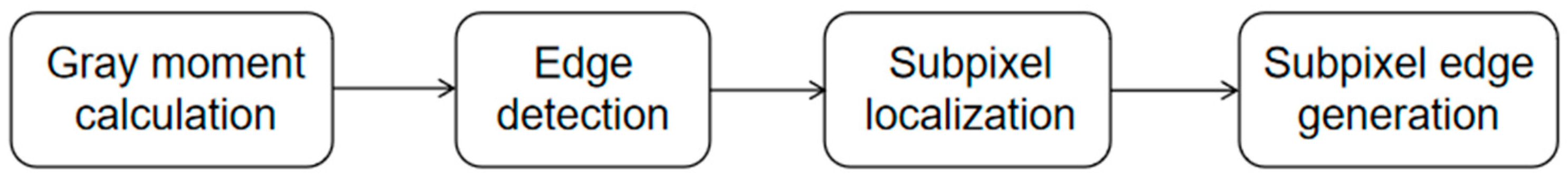
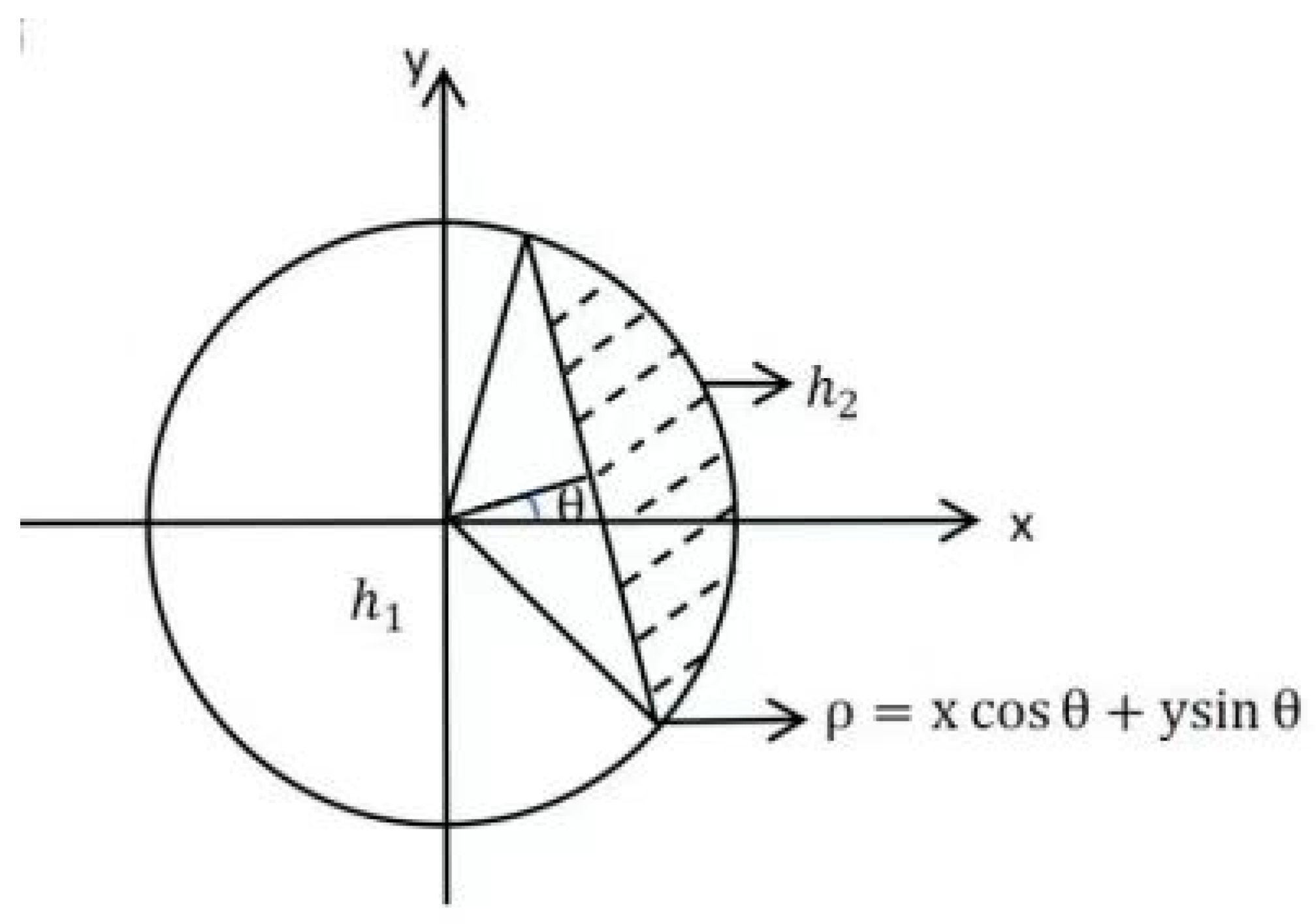
2.2.3. Gray Moment Sub-Pixel Edge Detection Algorithm

The gray moment sub-pixel edge detection method refers to the edge detection of an image based on the principle of gray moment invariance, i.e., it is assumed that the edge distribution in the actual image is consistent with the gray moments of the ideal step edge model [17]. A gray moment algorithm is applied to each edge point found by the improved Canny algorithm for sub-pixel level localization, and the edge map of the Canny algorithm is updated or corrected based on the results of the gray moment algorithm. The method flowchart is shown in Figure 1.

Calculation of Gray Moments

Gray moments are statistical quantities that describe the distribution of gray levels in an image and can be used to characterize the local features of an image. The first-order moments reflect the average gray value of the image, the second-order moments reflect the degree of gray fluctuation of the image, and the third-order moments reflect the degree of skewness of the image’s grayscale. The k-th order gray moment is defined as shown in Equation (3). In this paper, a $7\times 7$ operator template is used, i.e., $\mathrm{k}=7$.

$${\mathrm{m}}_{\mathrm{k}}={\sum }_{\mathrm{x}=1}^{\mathrm{N}}{\sum }_{\mathrm{y}=1}^{\mathrm{N}}\mathrm{I}\left(\mathrm{x},\mathrm{y}\right)·{\mathrm{x}}^{\mathrm{k}}·{\mathrm{y}}^{\mathrm{k}}$$

(3)

In the equation, $\mathrm{I}\left(\mathrm{x},\mathrm{y}\right)$ is the gray value of the image at point $\left(\mathrm{x},\mathrm{y}\right)$ and N is the size of the template.

The diagram of the ideal edge model for the gray moments is shown in Figure 2. The normalized parameter model $\mathrm{E}\left(\mathrm{x},\mathrm{y},\mathsf{\rho },\mathsf{\theta }\right)$ is jointly determined by four parameters, such as gray values of ${\mathrm{h}}_1$ and ${\mathrm{h}}_2$, edge position $\mathsf{\rho }$, and edge direction $\mathsf{\theta }$. The representation is shown in Equation (4).

$$\mathrm{E}\left(\mathrm{x},\mathrm{y},\mathsf{\rho },\mathsf{\theta }\right)=\left\{\begin{array}{c}{\mathrm{h}}_1, x\cos \mathsf{\theta }+\mathrm{y}\cos \mathsf{\theta }\le \mathsf{\rho }\\ {\mathrm{h}}_2, x\cos \mathsf{\theta }+\mathrm{y}\cos \mathsf{\theta }>\mathsf{\rho }\end{array}\right.$$

(4)

The proportion of pixel points with gray values of ${\mathrm{h}}_1$ and ${\mathrm{h}}_2$ to the total number of pixel points in the entire edge is set to ${\mathsf{\omega }}_1$ and ${\mathsf{\omega }}_2$, respectively, and ${\mathsf{\omega }}_1+{\mathsf{\omega }}_2=1$. So, the first three orders of gray moments ${\mathrm{m}}_{\mathrm{k}}$ can be expressed as Equation (5).

$${\mathrm{m}}_{\mathrm{k}}={\mathrm{h}}_1^{\mathrm{k}}{\mathsf{\omega }}_1+{\mathrm{h}}_2^{\mathrm{k}}{\mathsf{\omega }}_2 \mathrm{k}=1,2,3$$

(5)

Therefore, finding the gray moments of the first three orders is finding the weighted sum of the gray values of each pixel point with the expression shown in Equation (6). It should provide a concise and precise description of the experimental results, their interpretation, as well as the experimental conclusions that can be drawn.

$${\mathrm{m}}_{\mathrm{k}}={\sum }_{\mathrm{i}=1}^{\mathrm{N}}{\mathsf{\omega }}_{\mathrm{i}}{\mathrm{G}}_{\mathrm{i}}^{\mathrm{k}} \mathrm{k}=1,2,3$$

(6)

In the equation, ${\mathrm{G}}_{\mathrm{i}}$ is the gray value of the i-th pixel point in the unit circle; N is the size of the template; and ${\mathsf{\omega }}_{\mathrm{i}}$ is the weight value corresponding to the i-th pixel point.

The collation can be obtained as ${\mathsf{\omega }}_1$, ${\mathsf{\omega }}_2$, ${\mathrm{h}}_1$, and ${\mathrm{h}}_2$, with the formula shown in Equation (7).

$$\left\{\begin{array}{c}{\mathsf{\omega }}_1={\displaystyle \frac{1+\mathrm{s}\sqrt{1/\left(4+{\mathrm{s}}^2\right)}}{2}}\\ {\mathsf{\omega }}_2=1-{\mathsf{\omega }}_1\\ {\mathrm{h}}_1={\mathrm{m}}_1-\sigma \sqrt{{\displaystyle \frac{{\mathsf{\omega }}_2}{{\mathsf{\omega }}_1}}}\\ {\mathrm{h}}_2={\mathrm{m}}_1-\sigma \sqrt{{\displaystyle \frac{{\mathsf{\omega }}_1}{{\mathsf{\omega }}_2}}}\end{array}\right.$$

(7)

In the equation, $\mathsf{\sigma }=\sqrt{{\mathrm{m}}_2-{\mathrm{m}}_1^2}$, $\mathrm{s}={\displaystyle \frac{{\mathrm{m}}_3+2{\mathrm{m}}_1^3-3{\mathrm{m}}_1·{\mathrm{m}}_2}{{\mathsf{\sigma }}^3}}$.

Therefore, the edge position $\mathsf{\rho }$ and edge direction $\mathsf{\theta }$ can be obtained, and the expressions are shown in Equations (8) and (9), which are, respectively, as follows:

$$\mathsf{\rho }=\cos \mathsf{\theta }$$

(8)

$$\left\{\begin{array}{c}\sin \mathsf{\theta }={\displaystyle \frac{{\mathrm{y}}_0}{\sqrt{{\mathrm{x}}_0^2+{\mathrm{y}}_0^2}}}\\ \cos \mathsf{\theta }={\displaystyle \frac{{\mathrm{x}}_0}{\sqrt{{\mathrm{x}}_0^2+{\mathrm{y}}_0^2}}}\end{array}\right.$$

(9)

In the equation, ${\mathrm{x}}_0$, ${\mathrm{y}}_0$ are the grayscale center of gravity coordinates of the unit circle.

If the gray moments around a pixel point vary significantly, then the point is likely to be located on an edge. If $\left|{\mathrm{h}}_1-{\mathrm{h}}_2\right|>2\mathsf{\sigma }$ is satisfied, the point is considered to be an edge point. The location of the edge at the sub-pixel level is obtained by solving beyond Equation (10).

$$\mathrm{x}-{\displaystyle \frac{1}{2}}\sin 2\mathrm{x}-\mathrm{A}\mathsf{\pi }=0$$

(10)

In the equation, $\mathrm{A}=\min \left({\mathsf{\omega }}_1,{\mathsf{\omega }}_2\right)$.

3. RANSAC Algorithm

RANSAC is an algorithm for data fitting, also known as Random Sampling Consistency [18], especially in the presence of outliers in the data, which is effective in identifying interior points in the data and fitting the model based on these interior points [19]. The mathematical principle is as follows: for a total sample set of N, of which M data are interior points, the probability of taking an interior point each time is $\mathrm{P}=\mathrm{M}/\mathrm{N}$; K sample points are needed for the design calculation model; the probability of taking all the sample points in the interior point at one time is ${\mathrm{P}}^{\mathrm{K}}$, and then the probability that at least one sample point in the sampling points is an outlier is $1-{\mathrm{P}}^{\mathrm{K}}$.

If n samples are taken, the probability that all n samples include at least one out-of-bounds point is ${\left(1-{\mathrm{P}}^{\mathrm{K}}\right)}^{\mathrm{n}}$. Then, the rate of the opposite event of this event, i.e., the rate of a good model (where all the points taken are out-of-bounds) that has appeared at least once in the n samples, is $1-{\left(1-{\mathrm{P}}^{\mathrm{K}}\right)}^{\mathrm{n}}$. By the limit, it is known that when $\mathrm{n}\to \infty$, ${\left(1-{\mathrm{P}}^{\mathrm{K}}\right)}^{\mathrm{n}}\to 0$; the intuitive interpretation is that when the number of samples is sufficiently high, a good model is sure to appear.

In this paper, a small number of data points were randomly selected from all data points as parameters for an initial model, and then the consistency of the model with all data points was calculated. If the consistency exceeded a certain threshold, a feasible model was considered to be found. Next, the initial model was replaced with this feasible model and the consistency was recalculated. This process was performed iteratively until the stopping condition was met. During the iterative process, the fitting parameters were constantly updated and data points that were not consistent with the current model were eliminated. Taking this approach, the most appropriate circle can be found gradually.

The coordinates of the center of a uniquely determined circle and its mean radius can be calculated from the coordinates of three points in the plane. Three points, ${\mathrm{P}}_1\left({\mathrm{x}}_1,{\mathrm{y}}_1\right)$, ${\mathrm{P}}_2\left({\mathrm{x}}_2,{\mathrm{y}}_2\right)$, ${\mathrm{P}}_3\left({\mathrm{x}}_3,{\mathrm{y}}_3\right)$, are taken in the set of points and the difference, ${\mathrm{z}}_1$, ${\mathrm{z}}_2$, ${\mathrm{z}}_3$, which is the squared difference of the distance of each point from the origin, is calculated as shown in Equation (11).

$$\left\{\begin{array}{c}{z}_1={\mathrm{x}}_2^2+{\mathrm{y}}_2^2-{\mathrm{x}}_1^2-{\mathrm{y}}_1^2\\ z_2={\mathrm{x}}_3^2+{\mathrm{y}}_3^2-{\mathrm{x}}_1^2-{\mathrm{y}}_1^2 \\ z_3={\mathrm{x}}_3^2+{\mathrm{y}}_3^2-{\mathrm{x}}_2^2-{\mathrm{y}}_2^2 \end{array}\right.$$

(11)

The matrix A and the vector B are created. The matrix A reflects the relative positional relationship between the three points and the vector B is constructed from the previously calculated ${\mathrm{z}}_1$, ${\mathrm{z}}_2$, ${\mathrm{z}}_3$, after reduction by 0.5. A system of linear equations is constructed to solve for the coordinates of the center of the circle through matrix A and vector B, as shown in Equation (12).

$$\left\{\begin{array}{c} A=\left[\left({\mathrm{x}}_2-{\mathrm{x}}_1\right), \left({\mathrm{y}}_2-{\mathrm{y}}_1\right); \left({\mathrm{x}}_3-{\mathrm{x}}_1\right), \left({\mathrm{y}}_3-{\mathrm{y}}_1\right); \left({\mathrm{x}}_3-{\mathrm{x}}_2\right), \left({\mathrm{y}}_3-{\mathrm{y}}_2\right)\right]\\ B=0.5\ast \left[{\mathrm{z}}_1; {\mathrm{z}}_2; {\mathrm{z}}_3\right]\end{array}\right.$$

(12)

The principle of least squares is utilized to solve the optimal solution of the system of linear equations $\mathrm{Ax}=\mathrm{B}$. First, A is transposed and left multiplied to obtain $\left({\mathrm{A}}^{\prime }\ast \mathrm{A}\right)$, and then the left division operation is performed on the augmented matrix $\left({\mathrm{A}}^{\prime }\ast \mathrm{B}\right)$ to obtain the optimized center of the circle ${\mathrm{P}}_0$, with the expression shown in Equation (13).

$${\mathrm{P}}_0=\left({\mathrm{A}}^{\prime }\ast \mathrm{A}\right)\backslash {\mathrm{A}}^{\prime }\ast \mathrm{B}$$

(13)

The distances from the known center of the circle ${\mathrm{P}}_0$ to the three points ${\mathrm{P}}_1$, ${\mathrm{P}}_2$, ${\mathrm{P}}_3$, are calculated separately and the average of the three is taken as the final radius value; the expression is shown in Equation (14). It should be noted that the ideal calculation method should be to directly take the actual distance from any point to the center of the circle, and the average value is taken here to eliminate possible measurement errors.

$$\left\{\begin{array}{c} {\mathrm{R}}_1=\sqrt{{\left({\mathrm{P}}_0\left(1\right)-{\mathrm{P}}_1\left(1\right)\right)}^2+{\left({\mathrm{P}}_0\left(2\right)-{\mathrm{P}}_1\left(2\right)\right)}^2}\\ {\mathrm{R}}_2=\sqrt{{\left({\mathrm{P}}_0\left(1\right)-{\mathrm{P}}_2\left(1\right)\right)}^2+{\left({\mathrm{P}}_0\left(2\right)-{\mathrm{P}}_2\left(2\right)\right)}^2}\\ {\mathrm{R}}_3=\sqrt{{\left({\mathrm{P}}_0\left(1\right)-{\mathrm{P}}_3\left(1\right)\right)}^2+{\left({\mathrm{P}}_0\left(2\right)-{\mathrm{P}}_3\left(2\right)\right)}^2}\\ R=\left({\mathrm{R}}_1+{\mathrm{R}}_2+{\mathrm{R}}_3\right)/3\end{array}\right.$$

(14)

The obtained ${\mathrm{P}}_0$ also needs to be transposed to maintain the consistency of the data structure and to facilitate subsequent calls.

After completing all the iterations, the final edge position was determined based on all the fitted obtained circles. Specifically, for each fitted obtained circle, its distance from all data points in the image was calculated. Then, based on the size of the distance, whether each data point belongs to the edge was determined. If the distance of a data point was less than a certain threshold, it was considered as part of that edge. Finally, all data points belonging to the same edge were connected to form the final edge profile.

4. Experimental Objects and Analysis of Results

4.1. First Piston Component

The first piston part is an important part of the automobile braking system, which connects the brake cylinder and the brake. The performance of the first piston part directly affects the braking effect and safety performance of the automobile. Figure 3a shows the first piston component, which mainly detects the concentricity of the component spring and the outer wall, and the parts to be detected are shown in Figure 3b.

The images were acquired using a Hikvision MV-CU20-10GC color 12-megapixel CMOS face-matrix camera (Camera and Lens Sourcing with Changchun, China), with a resolution of 3036 × 4024, and the lens was a Hikvision MVL-KF1228M-12MPE-type lens with a focal length of 12 mm. The pixel accuracy in the horizontal and vertical directions was about 0.04 mm/pixel. The captured original image is shown in Figure 3b.

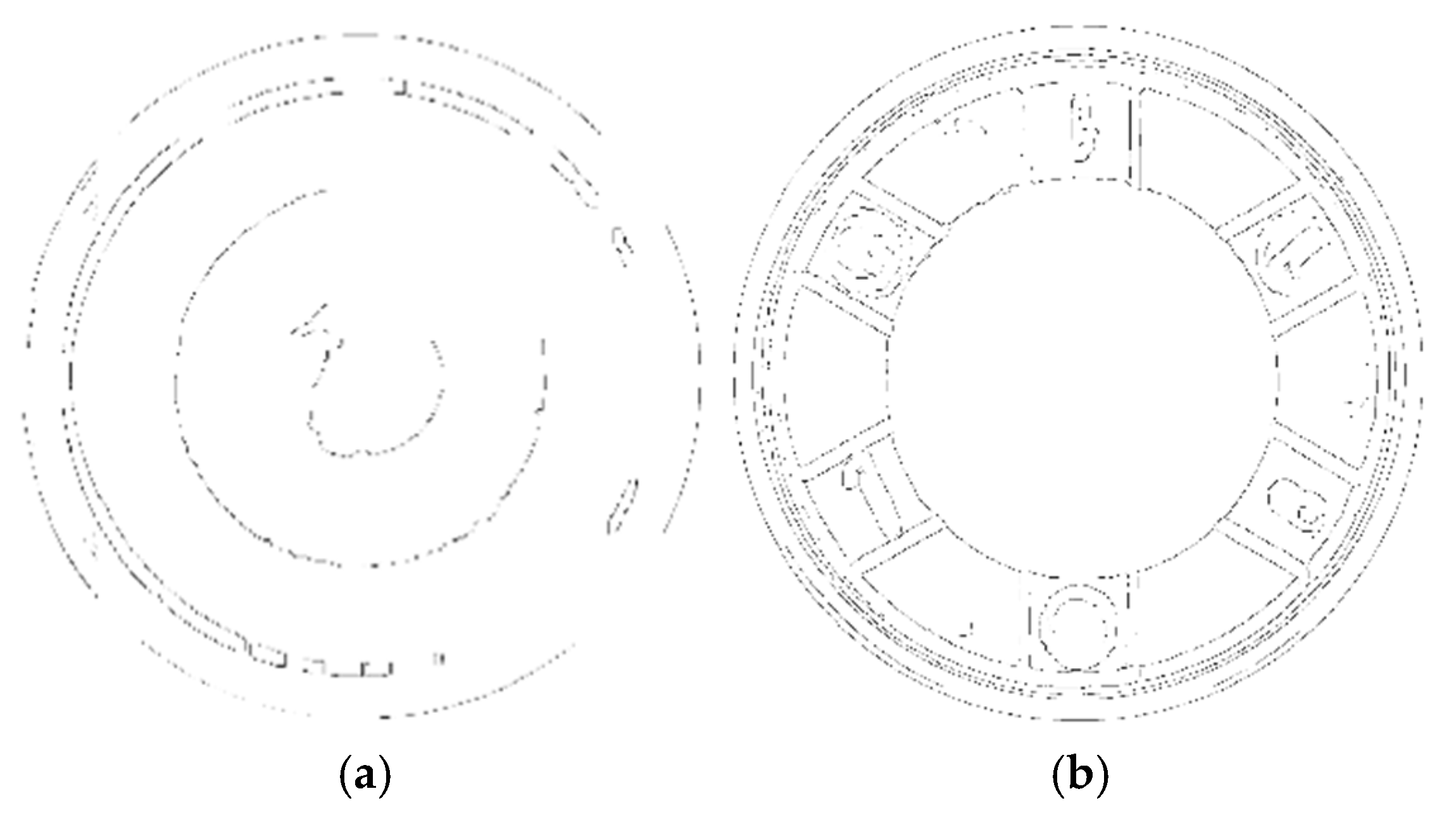
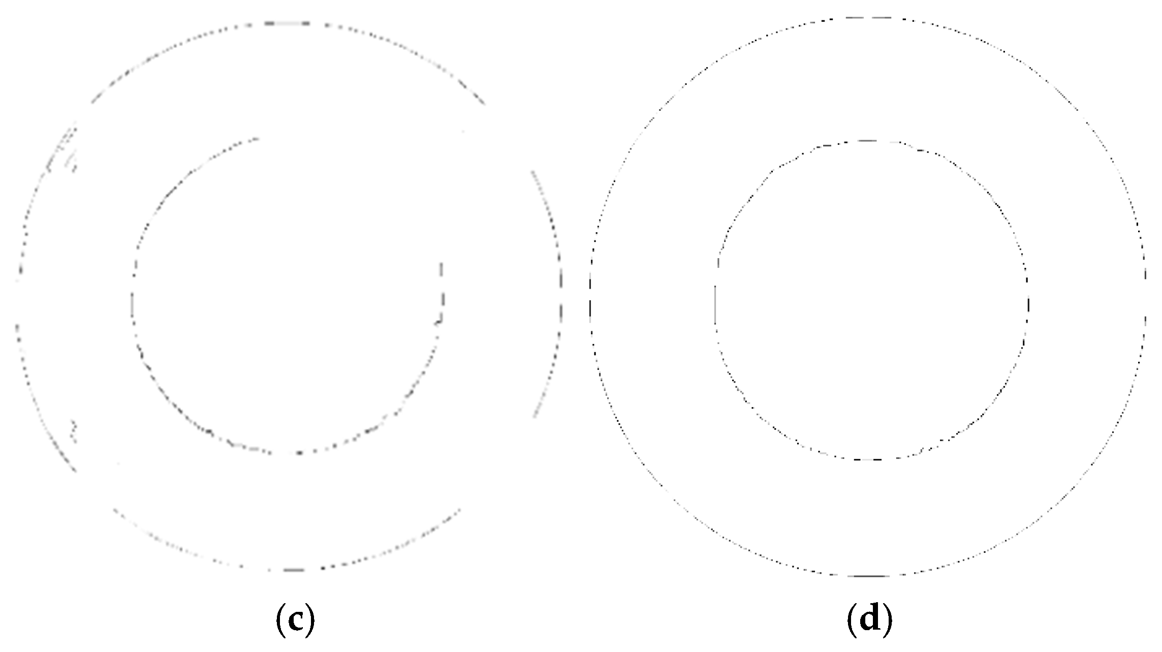
4.2. Edge Image Extraction

The traditional Canny algorithm and the improved Canny algorithm were applied to the concentricity detection of the first piston part using machine vision software, respectively. The extracted edges are shown in Figure 4a,b, and the inner and outer edge images were obtained by removing the interference points as shown in Figure 4c,d.

In Figure 4, it can be seen that the improved Canny algorithm edge detection algorithm has a good edge detection effect compared to the traditional Canny algorithm, which can retain the edge information in a more complete way, and can suppress the interference information near the edge line.

4.3. Analysis of Fitting Results

Five images were collected at the same location for the first piston part, and after extracting the edges using the improved Canny algorithm, the RANSAC algorithm was applied to fit them 10 times, respectively. The average value of the processed results was used as the detection value of concentricity of the first piston part after the improved algorithm. The average value of concentricity after the improved algorithm was obtained as 0.6475 mm and the data are shown in

Table 1. Fitting data (unit: mm).

Fitting Times	Original Image 1	Original Image 2	Original Image 3	Original Image 4	Original Image 5
First time	0.61872	0.66529	0.70329	0.63603	0.64464
Second time	0.78596	0.50514	0.65660	0.61228	0.59718
Third time	0.60205	0.64223	0.65253	0.61342	0.63857
Fourth time	0.72609	0.60871	0.63906	0.64046	0.40322
Fifth time	0.61912	0.64333	0.57418	0.61936	0.64323
Sixth time	0.66031	0.69923	0.60923	0.64542	0.65148
Seventh time	0.61843	0.60355	0.74016	0.61078	0.50514
Eighth time	0.66968	0.66274	0.63218	0.62800	0.89484
Ninth time	0.48028	0.71846	0.65326	0.76218	0.81706
Tenth time	0.65196	0.70728	0.68641	0.72281	0.65236
Average of ten times	0.64326	0.6456	0.65469	0.64907	0.64477
Overall average	0.6475

.

After extracting the edges using the traditional Canny algorithm, the same fitting was carried out, and the average value of concentricity was obtained as 0.6024 mm. The concentricity of this part was measured as 0.6405 mm using the coordinate measuring machine.

Taking the concentricity results measured by the coordinate measuring machine as the benchmark, the error value between the results of the traditional Canny algorithm and the benchmark is more than 0.035 mm, and the relative error is more than 5%, while the error value between the results of the improved Canny algorithm and the benchmark is within 0.01 mm, and the relative error is less than 0.5%, which verifies the validity of the improved Canny algorithm. The improved Canny algorithm reduces the concentricity error by 4%, which has high accuracy, and also proves that the improved Canny algorithm can obtain good solution accuracy in engineering applications.

5. Conclusions

Aiming at the problems of low efficiency of manual eye inspection and large subjective error in the concentricity detection of piston components, an improved Canny algorithm is proposed in this paper, which realizes high-precision automatic measurement through bilateral filtering, multi-scale analysis, and sub-pixel positioning optimization. The improved Canny algorithm is applied to the first piston component spring concentricity detection, and the results are compared with those of CMM. The main conclusions are as follows:

(1)

Algorithm improvement: The two-sided filter is applied to the Canny algorithm to solve the problem of image edge information loss during image preprocessing. Multi-scale analysis is introduced, an image pyramid is constructed, and the problem of detail loss caused by the Sobel operator in the Canny algorithm in a single-scale edge detection is solved, and thus the edge detection accuracy is improved.

(2)

Measurement performance: The concentricity detection error in the laboratory environment is less than ±0.01 mm, which meets the ISO 1938-2015 standard [20]. The deviation is reduced by 4%, and the repeatability is significantly better than manual detection.

(3)

Application potential: The method is compatible with the existing structure of the riveting machine testing station and has the engineering conditions of non-contact real-time measurement. It provides a reliable technical solution to replace manual eye inspection. The next step will be to carry out the adaptation verification of the production line.

References

1. Guo, Z. Research and Application of Circle Center Location Technology Based on Sub-Pixel Edge Detection. Master’s Thesis, Nanchang University, Nanchang, China, 2023. [Google Scholar] [CrossRef]
2. Zhu, L.; Zhang, J.; Dian, S. Design of coaxiality detection and fine-tuning system based on machine vision. J. Transducer Microsyst. Technol. 2022, 41, 94–98+102. [Google Scholar]
3. Wang, J.; Wang, X.; Cheng, B.; Dong, Z.; Zhai, Z.; Yang, L. Circle detection method based on moving sine fitting. J. China Instrum. 2021, 9, 56–61. [Google Scholar]
4. Peng, Y.; Xiao, J.; Mao, J.; Dai, Y.; Zhang, M. A multi-bottle-mouth positioning algorithm based on DBSCAN random circle detection. J. Electron. Meas. Instrum. 2021, 35, 43–52. [Google Scholar]
5. Zhao, C.; Fan, C.; Zhao, Z. The center of the circle fitting optimization algorithm based on the hough transform for crane. Appl. Sci. 2022, 12, 10341. [Google Scholar] [CrossRef]
6. Guo, J.; Yang, J. An iterative procedure for robust circle fitting. Commun. Stat.-Simul. Comput. 2019, 48, 1872–1879. [Google Scholar] [CrossRef]
7. Michałowska, M.; Rapiński, J.; Janicka, J. Tree position estimation from TLS data using hough transform and robust least-squares circle fitting. Remote Sens. Appl. Soc. Environ. 2023, 29, 100863. [Google Scholar] [CrossRef]
8. Ou, Y.; Deng, H.; Liu, Y.; Zhang, Z.; Ruan, X.; Xu, Q.; Peng, C. A fast circle detection algorithm based on information compression. Sensors 2022, 22, 7267. [Google Scholar] [CrossRef] [PubMed]
9. Zhou, X.; Wang, Y.; Zhu, Q.; Zhang, H.; Chen, Q. Circle detection with model fitting in polar coordinates for glass bottle mouth localization. Int. J. Adv. Manuf. Technol. 2022, 120, 1041–1051. [Google Scholar] [CrossRef]
10. Guo, S.; Yang, S.; Zhang, P. A circle detection algorithm based on ellipse removal. J. Image Process. Theory Appl. 2021, 4, 42–50. [Google Scholar]
11. Guo, P. Detection technology and application of parallelism and coaxiality of wind tower flanges based on laser measuring instrument. Electr. Appar. Ind. 2024, 10, 19–21+30. [Google Scholar]
12. Qing, Y.; Yanru, Z.; Wen, L. Design of Dynamic Parameter Acquisition Module of Field CMM. Meas. Control Technol. 2014, 33, 45–47+51. [Google Scholar]
13. Chen, Z.; Liu, Z. Research on underwater image edge detection method based on improved canny and gray-level moment. J. Agric. Equip. Veh. Eng. 2024, 62, 107–110+120. [Google Scholar]
14. van Kempen, G.M.P.; van Vliet, L.J.; Verveer, P.J.; van der Voort, H.T.M. A quantitative evaluation of image sharpness criteria for microscope autofocusing. IEEE Trans. Instrum. Meas. 2018, 67, 309–320. [Google Scholar]
15. Du, X.; Chen, D.; Ma, Z.; Liu, F. Improved image edge detection algorithm based on canny operator. Comput. Digit. Eng. 2022, 50, 410–413, 457. [Google Scholar]
16. Wang, D.; Tang, C.; E, S.; Gao, C.; Ge, B. Image edge detection based on guided filter Retinex and adaptive Canny. J. Opt. Precis. Eng. 2021, 29, 443–451. [Google Scholar] [CrossRef]
17. Zhang, M. Research on Sub-Pixel Edge Detection Technology. Master’s Thesis, Shenyang Ligong University, Shenyang, China, 2013. [Google Scholar]
18. Ren, Y.; Tu, D.; Han, S. Diesel engine cylinder liner size detection based on machine vision. J. Modul. Mach. Tool Autom. Manuf. Technol. 2020, 9, 151–153. [Google Scholar]
19. Shang, H.; Han, X.; Ji, C.; Peng, X. Application of circle fitting algorithm based on RANSAC in threaded hole detection. J. Mod. Manuf. Eng. 2024, 2, 112–119. [Google Scholar]
20. ISO 1938-2015; Geometrical Product Specifications (GPS)—Dimensional Measuring Equipment. ISO: Geneva, Switzerland, 2015.
Figure 1. Flowchart of the gray moment sub-pixel edge detection method.
Applsci 15 04397 g001
Figure 2. Diagram of the ideal edge model.
Applsci 15 04397 g002
Figure 3. (a) Piston component; (b) image of the part to be detected.
Applsci 15 04397 g003
Figure 4. The results of edge image extraction: (a) edges extracted by the traditional Canny algorithm; (b) edges extracted by the improved Canny algorithm; (c) inner and outer edge images obtained by removing interference points with the traditional Canny algorithm; and (d) inner and outer edge images obtained by removing interference points with the improved Canny algorithm.
Applsci 15 04397 g004aApplsci 15 04397 g004b