Article

The Effect of Green Areas on Urban Microclimate: A University Campus Model Case

by
Gülcay Ercan Oğuztürk
1,*,
Sude Sünbül
1 and
Cem Alparslan
2
1
Department of Landscape Architecture, Faculty of Engineering and Architecture, Recep Tayyip Erdoğan University, Rize 53020, Türkiye
2
Department of Mechanical Engineering, Faculty of Engineering and Architecture, Recep Tayyip Erdogan University, Rize 53100, Türkiye
*
Author to whom correspondence should be addressed.
Appl. Sci. 2025, 15(8), 4358; https://doi.org/10.3390/app15084358
Submission received: 6 February 2025 / Revised: 1 April 2025 / Accepted: 4 April 2025 / Published: 15 April 2025
(This article belongs to the Section Ecology Science and Engineering)

Abstract

:
Urbanization and the reduction of green spaces have significantly contributed to problems such as rising temperatures and declining air quality in urban areas. This study examines the impact of different types of green areas—broadleaved trees, coniferous trees, shrubs, and vines—on urban temperature regulation at the Recep Tayyip Erdoğan University Zihni Derin Campus. Surface temperature, humidity, ambient temperature, and wind speed measurements were collected using an infrared thermometer over a one-year period under various climatic conditions (August, October, January, and April) and at different times of the day (09:00 AM, 01:00 PM, and 05:00 PM). To quantitatively assess the cooling effect of each type of green area, a Response Surface Methodology (RSM) was applied, and a predictive formula was developed to estimate the cooling impact of various green areas under different environmental conditions. These formulated models enable the estimation of the temperature reduction provided by these four plant types based on different input parameters, achieving an accuracy of approximately 92% or higher without requiring direct measurements. The findings of this study provide a robust methodological framework and a practical tool for optimizing green space designs, mitigating urban heat island effects, and enhancing urban living comfort under various climatic conditions.

1. Introduction

The rapid urbanization occurring worldwide has led to a significant reduction in green areas [1,2,3] and the destruction of natural habitats, particularly in large cities [4,5,6,7]. This process has resulted in various environmental and social issues, such as increasing urban temperatures, declining air quality, and deteriorating living comfort [8,9,10,11,12]. The preservation and expansion of green areas [13,14,15] in urban spaces are crucial for sustainable urban planning [16,17,18]. In particular, the presence of green areas in highly urbanized regions contributes to balancing [19,20,21] urban ecosystems and directly impacts human health and quality of life. Furthermore, green areas play a critical role in regulating the urban microclimate [5,22,23,24,25]. Broadleaved trees, coniferous trees, shrubs, and vines not only provide aesthetic value but also reduce surface temperatures [26,27], mitigating the urban heat island effect [28,29,30,31]. The literature emphasizes that landscape areas designed with appropriate plant species can lower temperatures, improve microclimate conditions [23,32,33,34,35], and enable users to enjoy these spaces more comfortably for extended periods [9,36,37,38]. Additionally, green areas support ecosystem services by reducing carbon emissions, improving air quality, and contributing to rainwater management [39]. In addition to its ecological and climatic relevance, the role of green spaces in promoting landscape sustainability has gained increasing attention in recent studies. Green infrastructure contributes not only to environmental resilience but also to long-term sustainable urban development by integrating ecosystem services into land use planning [40,41,42].
Ensuring the sufficient presence of green areas in the physical structure of cities is essential for making urban life healthier and more sustainable. In this context, one of the critical urban spaces that should have extensive green areas is university campuses [43,44,45]. Universities are dynamic environments that cater to a broad range of users from different age groups, including students, academics, and other campus residents who spend a significant portion of their time in these spaces. The presence of green areas on campuses offers substantial advantages in terms of both environmental sustainability and the psychological and physical well-being of users [30,46,47]. The optimization of plant-based designs on university campuses should be carried out not only for aesthetic concerns but also by considering functional benefits. Selecting plant species suitable for climatic conditions, implementing shading strategies, and incorporating ecological landscaping arrangements improve the microclimate while enhancing the quality of life for campus users [48,49,50,51]. These spaces are vital urban components that enhance individuals’ interaction with nature, supporting their academic and social lives. Therefore, in today’s rapidly urbanizing world, preserving and effectively planning green areas on university campuses should be regarded as an integral part of the sustainable urbanization approach.
While numerous studies have explored the role of urban green spaces in mitigating surface temperature and reducing the Urban Heat Island (UHI) effect, most have primarily relied on remote sensing indicators such as NDVI or land cover classifications without differentiating among plant species or accounting for their biophysical traits. For instance, refs. [52,53] reported strong inverse relationships between vegetation cover and surface temperature in cities like Chicago and Tel Aviv, yet they did not assess the differential cooling effects of individual plant types. Similarly, ref. [54] demonstrated the efficiency of green roofs in Bangkok’s tropical climate but without reference to species-specific physiological properties.
In contrast, this study contributes a more nuanced analysis by incorporating species-level variation (broadleaf, conifers, shrubs, and ivy) and focusing on functional traits such as Leaf Area Index (LAI), canopy density, and surface albedo. Refs. [55,56] emphasized the role of vertical canopy gradients and leaf-sapwood ratios in regulating plant respiration and energy exchange, while ref. [57] highlighted how spatial variation in LAI correlates with thermal performance in urban parks. Furthermore, studies by [58,59] stressed the importance of vegetation morphology and structure in seasonal temperature variation yet lacked species-level field assessments across varying microclimatic conditions.
By integrating in situ surface temperature measurements and plant-specific morphological data, this study offers a localized yet transferable model for understanding vegetation–climate interactions in humid subtropical zones. In doing so, it addresses a significant gap in the literature by moving beyond generalized vegetation classifications and emphasizing the need for plant-specific, trait-based approaches in designing effective urban greening strategies [60,61,62]. This study aims to examine the impact of different types of green areas (broadleaved trees, coniferous trees, shrubs, and vines) on urban temperature regulation at Recep Tayyip Erdoğan University Zihni Derin Campus, located in Rize. Surface temperature, humidity, ambient temperature, and wind speed measurements were conducted over a one-year period under various climatic conditions (August, October, January, and April) and at different times of the day (09:00 AM, 01:00 PM, and 05:00 PM). Surface and ambient temperature measurements were taken using an infrared thermometer, humidity measurements were conducted with a hygrometer, and wind speed measurements were taken with an anemometer. Within the scope of the study, the temperature regulation effect of each type of green area was quantitatively assessed, and a regression analysis was conducted to develop a predictive model capable of estimating the cooling impact of these areas under different environmental conditions. This model highlights the strong cooling effects of broadleaved and coniferous trees while also demonstrating the complementary roles of shrubs and vines. These findings provide a scientific foundation for mitigating urban heat island effects, improving urban living comfort, and supporting sustainable urban design. By emphasizing the importance of green areas in urban planning, this study encourages the enhancement of plant-based designs with the potential to improve the microclimate.
Thus, this study fills a critical knowledge gap by providing a trait-based, species-specific approach to urban microclimate regulation, particularly in humid subtropical contexts.

2. Materials and Methods

This study was conducted within the boundaries of Recep Tayyip Erdoğan University Zihni Derin Campus, located in Rize, Turkey (Figure 1). The campus provides a suitable environment for examining surface temperature variations due to its diverse topographic structure, varying levels of land use intensity, and the presence of different types of vegetative areas. Within the scope of the study, locations dominated by different types of green spaces, including broad-leaved trees, coniferous trees, shrubs, and ivy, were selected. The locations had broad-leaved plants (Salix babylonicaPrunus serrulataCercis siliquastrum), Coniferous Plants (Thuja occidentalisCedrus deodoraJuniperus chinensis), shrubs (Nandina domesticaElaeagnus pungensGrevilla rosmarinifolia), and ivies, (Hedera helixHedera hibernicaHedera helix).
Although the study area, Recep Tayyip Erdoğan University Zihni Derin Campus, may appear geographically specific, its selection is methodologically and climatically justified. Located in Rize, the campus resides within a humid subtropical climate zone characterized by high precipitation, moderate temperatures, and rich vegetation diversity—conditions comparable to other urban settings that experience thermal stress due to climate change. Moreover, the campus includes a range of green typologies (broadleaved trees, conifers, shrubs, ivy), topographic variability, and user activity patterns, which provide a suitable context for investigating vegetation–climate interactions under realistic conditions [63,64]. Previous studies have shown that green infrastructure implementations in diverse climate zones, such as Bangkok and Addis Ababa, can significantly reduce surface temperatures and improve urban comfort, highlighting the transferability of such research findings [54,65]. University campuses, widely used in landscape and ecological planning studies, serve as controlled yet dynamic urban environments, offering valuable data on vegetation–climate interactions [66,67]. Hence, the selected study area provides both accessibility and ecological relevance, making it an appropriate model for broader applications in urban green infrastructure planning. To ensure methodological consistency and environmental representativeness, a purposive sampling strategy was adopted to select the vegetated areas within the campus. Each green area type (broadleaved trees, conifers, shrubs, and ivy) was chosen based on distinct structural and physiological features, such as canopy density, height, and coverage area. The measurement locations were selected to capture a range of microclimatic conditions, including shaded, semi-shaded, and sun-exposed zones, thereby enabling comparative evaluation of their thermal regulation effects. Additionally, sampling sites were distributed across varying elevations and orientations to reflect the topographical diversity of the campus. This stratified approach allowed the study to assess how specific plant groups influence AT under different spatial and temporal contexts. The repeated measurement design and standardized device calibration ensured data reliability and reproducibility across all sampling periods.
The effects of different types of green spaces, including broad-leaved trees, conifers, shrubs, and ivy, on surface temperatures are being examined. The selected areas were determined in a way that ensures consistency in environmental variables such as shading, wind effects, and distance from buildings. An infrared thermometer (Testo 830-T2 (Testo, Titisee-Neustadt, Germany) and accuracy: ±1.5 °C (between 0 and 500 °C)) was used to measure surface and ambient temperatures. This device utilizes infrared (IR) sensing technology to perform non-contact measurements, accurately determining surface temperature. A hygrometer (Extech 445815 Humidity Meter (Extech Instruments, Nashua, NH, USA), and accuracy: ±3% RH (relative humidity)) was used to determine humidity levels, providing precise data by measuring the relative humidity in the environment. To measure wind speed, an anemometer (Kestrel 3000 Pocket Weather Meter (Kestrel Instruments, Boothwyn, PA, USA), accuracy: ±3% of reading, and range: 0.4 to 40 m/s) was employed, offering reliable data by assessing airflow velocity. To ensure measurement accuracy, all devices were calibrated and compared with reference values. Within the campus, locations with broad-leaved trees, conifers, shrubs, and ivy in sun-exposed areas were identified. Measurement points were systematically determined in these areas and recorded by marking each point on a map. This step was crucial for ensuring the continuity and consistency of the measurements (Figure 2). All instruments were inspected prior to each data collection session to ensure battery levels and sensor cleanliness. Measurements were conducted under stable atmospheric conditions to minimize data variability. Potential measurement errors due to human handling were minimized by holding each device at a consistent height (150 cm) and angle during the fieldwork.
The selection of the months (January, April, August, and October) was based on the representation of four distinct seasons in the humid subtropical climate of Rize, which allowed for capturing seasonal variation in microclimatic parameters. Similarly, the chosen time points (09:00, 13:00, and 17:00) represent the morning, midday, and late afternoon periods, respectively—each with different levels of solar radiation and thermal exposure. This temporal structure is consistent with prior studies investigating the thermal performance of green spaces across diurnal cycles [68,69] and is further supported by recent findings that highlight the importance of time-based variation in vegetation–climate interactions [70,71]. These time intervals help assess the dynamic thermal behavior of different vegetation types throughout the day under varying atmospheric conditions.
Measurements were conducted in January (winter), April (spring), August (summer), and October (autumn). Data collection took place at three different times of the day: 09:00 (morning), 13:00 (noon), and 17:00 (evening). To better evaluate temperature variations throughout the day, three repeated measurements were taken at each measurement point, and the average values were used. Before starting the measurement process, the calibration of the measurement devices and the condition of their batteries were checked. Upon arrival at the designated measurement locations, any accumulated dust, leaves, or water puddles on the surface were cleared. During the measurement process, the infrared thermometer was held at approximately 150 cm height and positioned perpendicular to the surface (Figure 2a). Three repeated measurements were taken at each point, and the averages were recorded. For humidity measurements, the hygrometer was held at approximately 150 cm height to ensure a representative assessment of ambient conditions (Figure 2b). Three repeated measurements were taken at each measurement point, and the average values were recorded. The humidity levels in different areas (e.g., shaded and sun-exposed regions) were compared. For wind speed measurements, the anemometer was held at approximately 150 cm height and exposed directly to the airflow for the most accurate readings (Figure 2c). Three repeated measurements were taken at each measurement point, and the average values were recorded. The variations in wind speed across different areas were analyzed.

Data Recording and Preliminary Analysis

The field data collected during the study were systematically recorded and prepared for the analysis process. Measurement results were stored using Excel spreadsheets or standardized data collection forms to minimize error rates and ensure data consistency. To enhance data reliability, environmental factors encountered during the measurement process (e.g., rainfall, wind speed variations, and solar radiation intensity) were documented in detail. Preliminary analysis was conducted to assess the validity of the collected data. In this context, abnormal values observed for specific variables (e.g., measurements significantly deviating from the average) were identified and excluded from the analysis to improve statistical reliability. To assess data quality prior to analysis, potential outliers were examined for all key variables used in the model, including AT, M, WS, A, and T. Outlier detection was based on the interquartile range (IQR) method, where any data points falling below Q1 − 1.5 × IQR or above Q3 + 1.5 × IQR were flagged as potential outliers. These thresholds were applied separately for each vegetation type and variable. Although outliers were identified, no data points were excluded from the model unless supported by clear evidence of measurement error (e.g., sensor malfunction). Additionally, preprocessing steps were applied, considering calibration processes of measurement devices and potential recording errors.
For detailed statistical analysis, RSM Regression Analysis was performed. RSM is a statistical approach based on mathematical models used in experimental designs to determine the relationship between input and output variables. In this technique, the Central Composite Design (CCD) was used as the experimental design approach, allowing for the evaluation of linear effects resulting from second-order interactions between different input variables [4,7]. A second-degree mathematical model was used to calculate the response resulting from interactions (Equation (1)).
Y = a 0 + i = 1 k b i X i + i j k b i j X i j + i = 1 k b i i X i 2 +   n
In this analysis process, T was used as the dependent variable, while measurement A, WS, AT, and M were used as independent variables. This analysis aimed to determine the effects of independent variables on surface temperature and develop a predictive model. The model was designed to estimate surface temperatures based on different surface types and environmental conditions. The obtained regression model was subjected to validation tests using field data to assess the agreement between predicted and actual surface temperature measurements. This validation process was conducted to test the reliability of the model and improve its accuracy against varying environmental factors.

3. Results and Discussion

3.1. Seasonal Variations, the Impact of Green Areas, and Microclimate Improvement Potential

The study has identified that vegetative areas (broadleaved trees, coniferous trees, shrubs, and vines) play a crucial role in regulating [72,73] the urban microclimate [23,33,34,74].
January (winter season): During winter, surface temperatures in vegetative areas were measured between 2 and 5 °C, demonstrating that green areas maintain their thermal regulation effect throughout the year.
April (spring season): In spring, surface temperatures in vegetative areas ranged between 20 and 30 °C. The shading effect of broadleaved trees was particularly evident in this period.
August (summer season): In summer, surface temperatures in green areas were recorded between 20 and 30 °C. Broadleaved trees and shrubs stood out for their strong shading properties.
October (autumn season): During autumn, surface temperatures in vegetative areas ranged between 15 and 25 °C, further confirming that green areas have a year-round temperature-regulating potential. It has been determined that green areas exhibit temperature regulation functions in all seasons [75,76,77], particularly mitigating rising temperatures in summer [36,78,79] and reducing the urban heat island effect [80,81,82]. This finding underscores the necessity of prioritizing the preservation and expansion of green areas in urban planning processes.

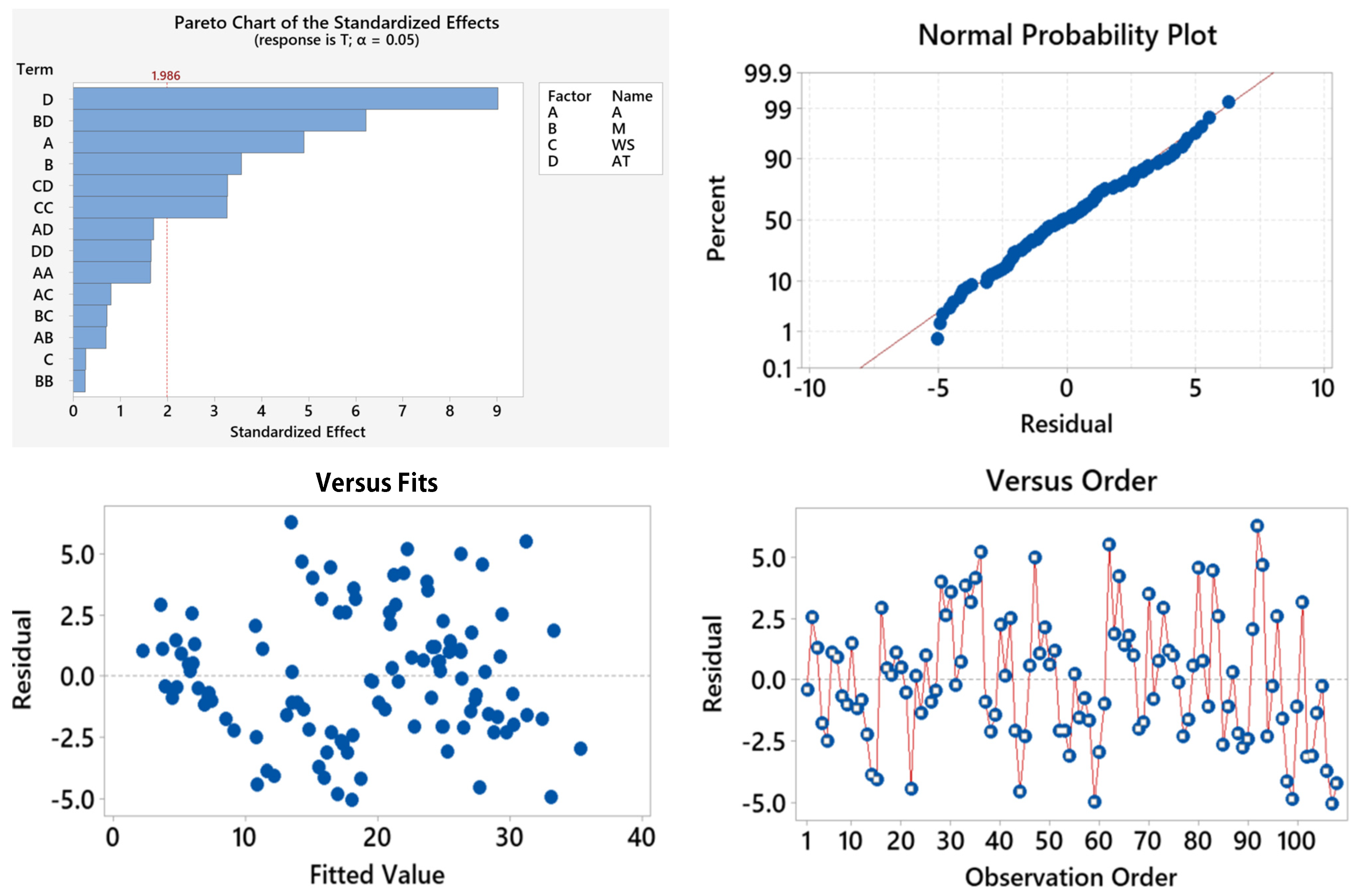
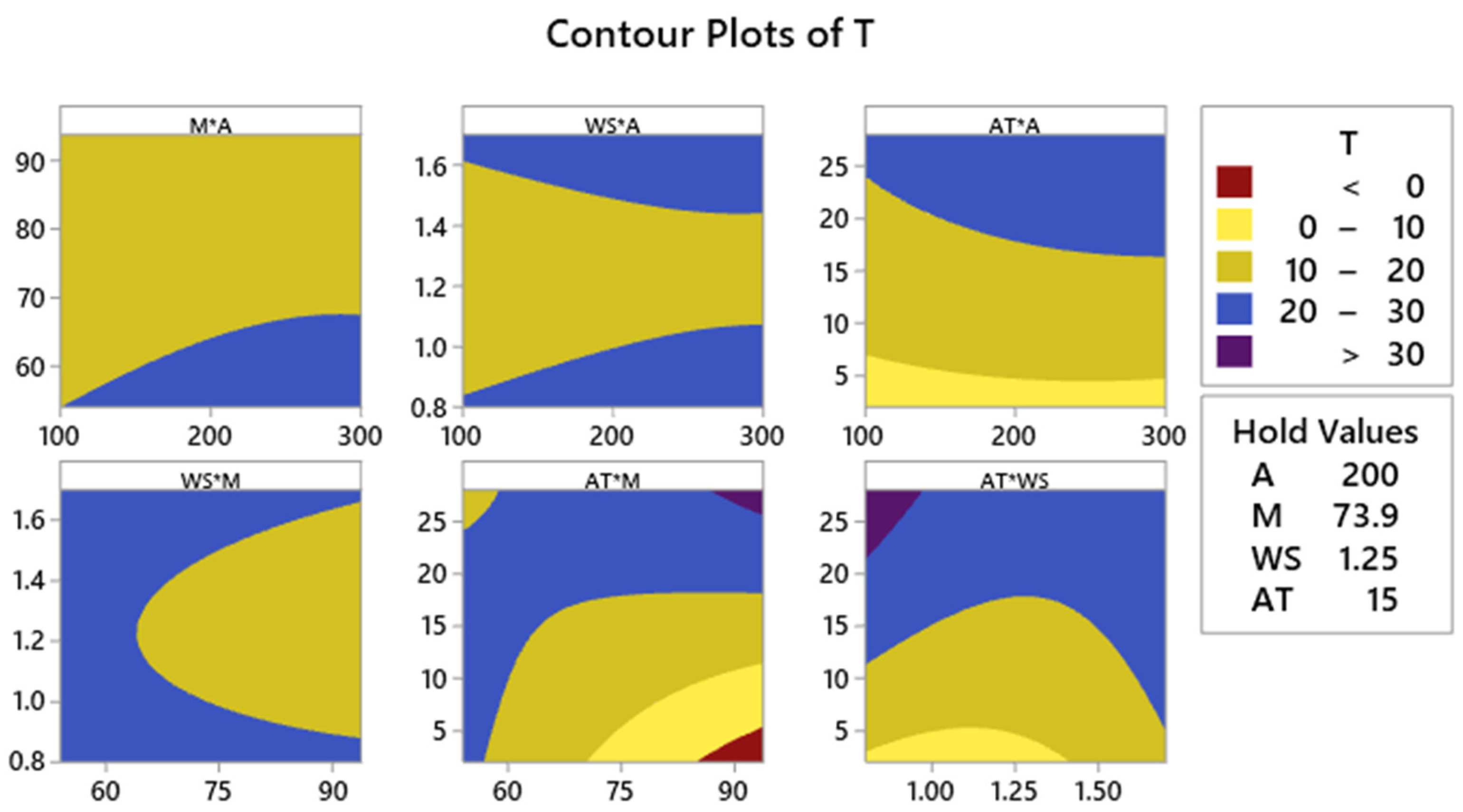
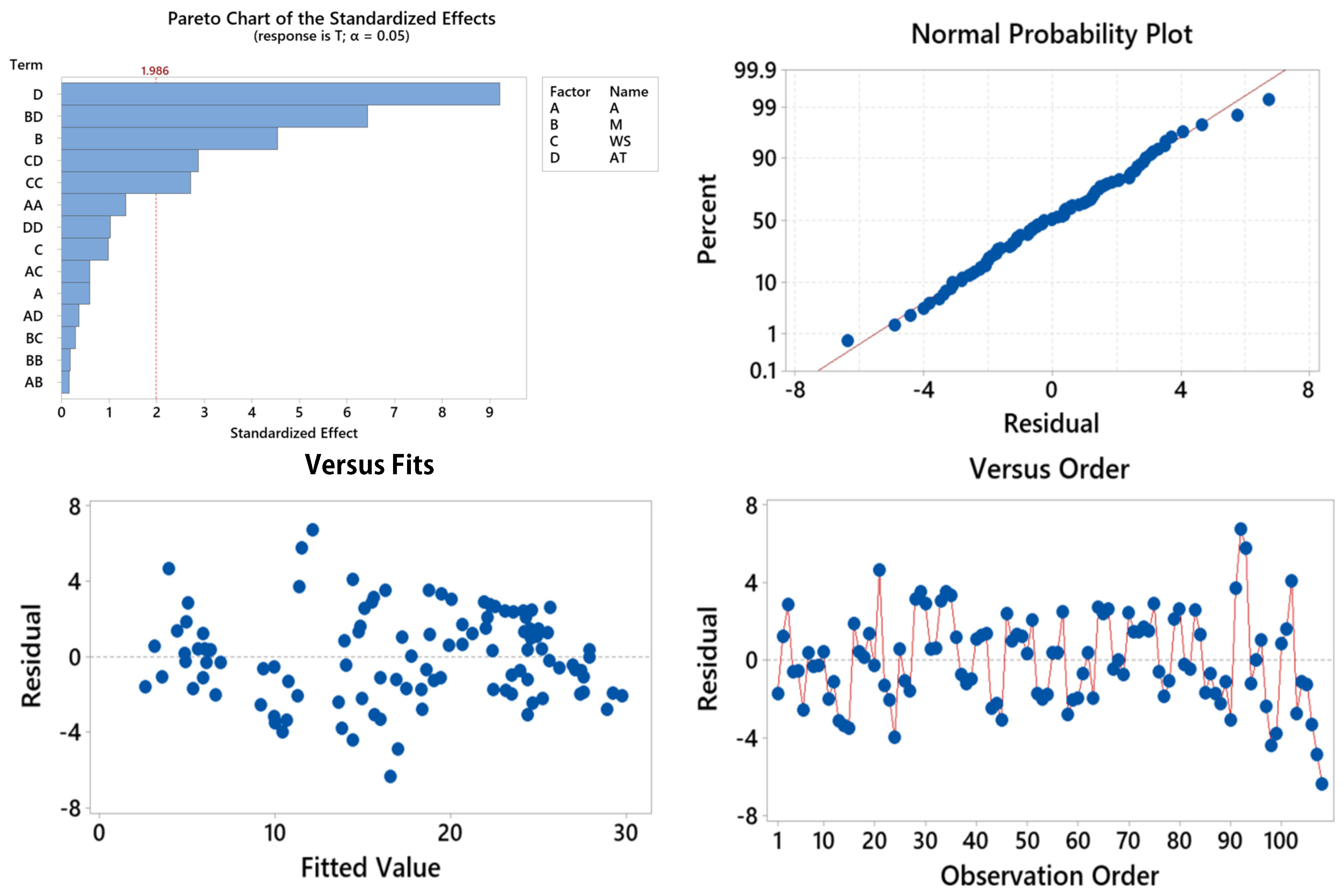
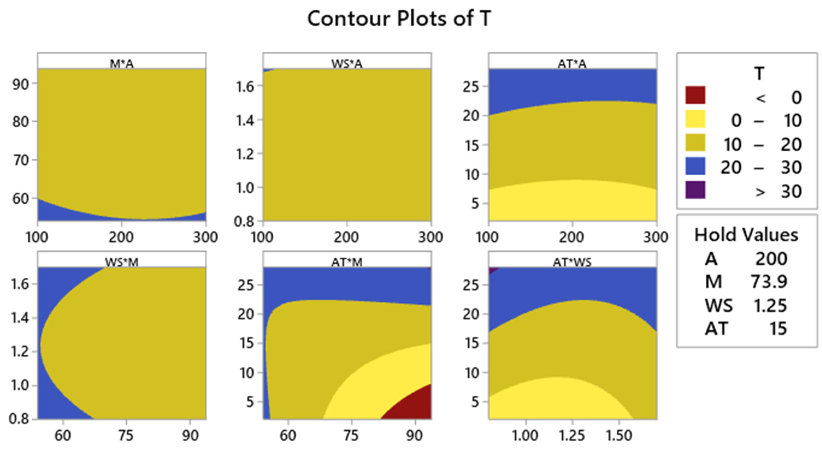
3.2. Regression Model and Applicability

The ANOVA results presented in Table 1 indicate that the RSM model developed in this study is statistically significant. The model’s high F-value (519.917) and low p-value confirm that the independent variables have a strong influence on the response variable. The linear terms explain 85.59% of the total variance, with the AT factor contributing 70.14%, followed by the M factor (7.96%). Quadratic terms account for 4.46%, while two-factor interactions contribute 3.48%. Among these, the interaction between M and AT (F = 227.222, 2.91%) emerges as the most significant. The low error rate (6.49%, Adj SS = 505.21) further supports the reliability of the model.
In conclusion, the ANOVA analysis indicates that AT and M are the most decisive factors affecting the response variable. The model demonstrates a strong fit in predicting the dependent variable. To enhance the reliability and robustness of the regression model developed in this study, a five-fold cross-validation technique was employed. The dataset was randomly partitioned into five equal subsets. In each iteration, four subsets were used to train the model, while the remaining subset served as the validation set. This process was repeated five times, ensuring that each subset was used for validation once. The average performance metrics—including R2, RMSE (Root Mean Square Error), and MAE (Mean Absolute Error)—were computed across all folds to evaluate model accuracy and generalizability. The use of cross-validation not only mitigated overfitting but also provided a comprehensive assessment of the model’s predictive power under varying environmental conditions. The results indicated high consistency across folds, confirming the robustness of the model in estimating surface temperature responses to different vegetation types.
Regression Equation in Uncoded Units
T = 50.3 + 0.1284 A + 0.187 M − 64.4 WS − 0.984 AT − 0.000222 A×A − 0.00640 M×M + 26.43 WS×WS − 0.01974 AT×AT − 0.000407 A×M − 0.00015 A×WS + 0.000342 A×AT + 0.041 M×WS + 0.03551 M×AT − 0.264 WS×AT
Table 1, Analysis of Variance (ANOVA) for Leafy Plants, showing the influence of four independent variables—surface area (A), humidity (M), wind speed (WS), and ambient temperature (AT)—on surface temperature (T). The model explains 93.51% of the total variance, with AT being the dominant factor (70.14%), followed by M (7.76%) and A (1.69%). Significant quadratic and two-way interactions were also observed, especially between M and AT (F = 227.22). The low p-values (<0.05) indicate the model’s strong statistical significance, while the low error contribution (6.49%) confirms the robustness of the model.
In Figure 3 and Figure 4, the effect of the plant’s measurement area, ambient humidity, wind speed, and temperature on the leafy plant is illustrated using a Pareto chart and contour plot. Upon examining the figure, it is observed that ambient temperature has a significant impact on the temperature of the leafy plant while also notably influencing humidity levels.
Figure 3, Pareto chart and residual analysis for Leafy Plants. The Pareto chart identifies the standardized effects of main and interaction terms, with AT, M, and the interaction M×AT being the most influential. The normal probability plot shows residuals aligning closely along the diagonal, indicating normality. The residuals vs. fitted values and residuals vs. order plots confirm randomness and independence, supporting the model’s homoscedasticity and predictive validity.
Figure 4, Contour plots showing the interaction effects between independent variables on T for Leafy Plants. AT and M interactions yield the most distinct thermal gradients, especially in the AT×M and M×AT plots, where red and yellow zones indicate optimal cooling potential. Hold values used in plots are A = 200, M = 73.9, WS = 1.25, AT = 15. These visualizations confirm that T response varies depending on the combination of microclimatic conditions and plant characteristics, offering guidance for targeted landscape interventions.
The experimental results indicate that the AT, M×AT, M, and A factors have the highest impact. Residual analysis confirms that the model follows a normal distribution and exhibits high predictive power due to the randomly distributed residuals. The Pareto chart reveals that some interactions, such as M×AT and A×A, may be more influential than individual factors. Contour plots show that optimal results are achieved in the red and yellow regions. Overall, the model is reliable, and the identified factors and interactions are critically important for optimization.
According to Table 2, the RSM model is statistically significant (F = 70.58, p < 0.001). Linear terms play a substantial role in explaining the model (10.89%), with AT being the most prominent factor (7.52%), followed by M (2.21%). Quadratic terms account for 2.87% of the total variance, while two-factor interactions contribute 4.88%. Among these, the AT×M interaction (F = 38.54, 3.56%) emerges as the most significant. The low error rate (8.6%, Adj SS = 726.67) further supports the reliability of the model.
Regression Equation in Uncoded Units
T = 91.7 + 0.0376 A − 0.955 M − 54.1 WS −1.208 AT − 0.000093 A×A + 0.00159 M×M + 29.83 WS×WS − 0.01107 AT×AT + 0.000228 A×M − 0.0094 A×WS + 0.000802 A×AT − 0.088 M×WS + 0.04088 M×AT − 0.772 WS×AT
Table 2, ANOVA results for Coniferous Plants. The model explains 91.40% of the total variance in T. The most influential variable is AT, with A 69.82% contribution, followed by M at 4.65% and A at 2.94%. While WS alone is statistically insignificant (p = 0.799), its interaction with AT (WS×AT) and the M×AT interaction is highly significant, with F-values of 10.71 and 38.54, respectively. These interactions suggest that combined microclimatic conditions are more impactful than individual variables. The low error rate (8.60%) supports the robustness and reliability of the RSM model.
The graphical analyses in Figure 5 and Figure 6 indicate that the model follows a normal distribution and that the residuals are randomly distributed. The Pareto chart has identified AT, M×AT, M, and A as the most influential factors. Contour plots show that the optimal response variable is obtained in the red and yellow regions, with AT and M factors being the key determinants. In conclusion, the AT factor is the strongest variable, and its interaction with M enhances the predictive power of the model.
Figure 5, Pareto chart and residual diagnostics for Coniferous Plants. The Pareto chart highlights AT, M, and the interaction term M×AT as the most significant predictors of T variation. The normal probability plot shows a close alignment to the theoretical distribution, indicating normality. The Versus Fits and Versus Order plots exhibit randomly scattered residuals without obvious patterns, confirming the assumptions of independence and constant variance (homoscedasticity) and validating the statistical reliability of the model.
Figure 6, Contour plots of T for Coniferous Plants, illustrating interaction effects among A, M, WS, and AT. The most prominent interactions appear in the AT×M and M×AT plots, where red and yellow zones indicate stronger cooling effects. The AT×WS plot also shows notable gradients, indicating how AT modulates the influence of WS. These plots provide visual evidence for the nonlinear and interactive behavior of environmental variables, underscoring the importance of multivariate considerations in green infrastructure planning.
According to Table 3, the RSM model is statistically significant (F = 69.34, p < 0.001). Linear terms explain a significant portion of the model’s variance (9.96%), with AT being the strongest variable (7.98%), followed by M (1.93%). Quadratic terms account for 1.96% of the total variance, while two-factor interactions contribute 4.82%. The M×AT interaction (F = 41.35, 3.88%) has been identified as the most significant interaction. The model exhibits a low error rate (8.74%, Adj SS = 592.22) and is considered reliable.
Regression Equation in Uncoded Units
T = 86.6 + 0.0162 A − 0.887 M − 43.9 WS − 1.281 AT − 0.000070 A×A + 0.00101 M×M + 22.36 WS×WS − 0.00620 AT×AT + 0.000046 A×M + 0.0062 A×WS + 0.000152 A×AT − 0.032 M×WS + 0.03822 M×AT − 0.612 WS×AT
Table 3, ANOVA results for shrubs. The model explains 91.26% of the total variance in T. Among the linear factors, AT is the most dominant (70.34%), followed by M (5.50%) and WS (7.75%). However, A has a negligible effect (0.02%, p = 0.559). Significant interactions include M×AT (F = 41.35) and WS×AT (F = 8.26), confirming the importance of combined climatic effects. The model’s reliability is supported by a low error contribution (8.74%) and statistically significant interaction terms.
According to Figure 7 and Figure 8, the model conforms to a normal distribution, and the residuals are randomly distributed. The Pareto chart identifies AT, M×AT, and M as the most influential factors. Contour plots indicate that the optimal response variable is achieved in the red and yellow regions, with AT and M factors being the key determinants. In conclusion, AT is the most significant independent variable, and its interaction with M enhances the predictive power of the model.
Figure 7, Pareto chart and residual analysis for shrubs. The ambient AT and its interaction with M (M×AT) are identified as the most impactful predictors of T. The normal probability plot confirms the normality of residuals, while the Versus Fits and Versus Order plots show randomly scattered residuals, verifying the assumptions of homoscedasticity and independence. These diagnostics validate the statistical robustness and predictive performance of the model.
Figure 8, Contour plots of T for shrubs, showing how the T varies with the interaction of environmental factors. The most significant interactions—AT×M and M×AT—demonstrate strong gradients with visible red and yellow zones, indicating higher cooling effects. The influence of WS is also observable in the WS×AT and WS×WS plots. These graphical representations reinforce the model’s findings by visually depicting how different variables synergistically regulate microclimate conditions in shrub-covered areas.
According to Table 4, the RSM model is statistically significant (F = 81.76, p < 0.001). Linear terms explain a large portion of the model’s variance (12.48%), with AT being the strongest variable (9.68%), followed by M (2.83%). Quadratic terms account for 2.34% of the total variance, while two-factor interactions contribute 4.00%. The M×AT interaction (F = 41.04, 3.31%) has been identified as the most significant interaction. The model exhibits a low error rate (7.51%, Adj SS = 591.98) and is considered reliable.
Regression Equation in Uncoded Units
T = 108.7 − 0.0521 A − 1.185 M − 47.7 WS − 1.575 AT + 0.000114 A×A + 0.00225 M×M + 21.48 WS×WS + 0.00587 AT×AT + 0.000076 A×M + 0.0040 A×WS − 0.000579 A×AT + 0.009 M×WS + 0.03806 M×AT − 0.446 WS×AT
Table 4, ANOVA results for Vines. The model explains 92.49% of the total variance in T. Among the linear factors, AT shows the highest contribution (71.45%, p < 0.001), followed by M (7.87%). A and WS are statistically insignificant on their own. The M×AT interaction (F = 41.00, p < 0.001) and WS×AT interaction (F = 4.38, p = 0.039) are the most prominent two-way effects. The model demonstrates high reliability with a low error rate (7.51%), indicating a strong fit between observed and predicted values.
When analyzing the graphs in Figure 9 and Figure 10, it is observed that the model conforms to a normal distribution and that the residuals are randomly distributed. The Pareto chart reveals that the AT, M×AT, and M factors have the highest impact. The contour plots indicate that the optimal response variable is obtained in the red and yellow regions, highlighting the determining influence of the AT and M factors. In conclusion, the AT factor is the most significant independent variable, and its interaction with M enhances the predictive power of the model.
Figure 9, Residual diagnostics and Pareto chart for Vines. The Pareto chart reveals that AT, M, and the interaction term M×AT have the strongest standardized effects on T. The normal probability plot shows residuals closely following the expected trend, validating normal distribution. Additionally, the Versus Fits and Versus Order plots confirm the randomness and independence of residuals, supporting the assumption of homoscedasticity and enhancing the model’s statistical credibility.
Figure 10, Contour plots for Vines, displaying the combined effects of environmental variables on T. The M×AT and AT×M plots show strong gradient shifts in color, indicating effective cooling performance through synergistic humidity–temperature interactions. Plots such as WS×AT also demonstrate localized thermal variations, especially in transitional zones. Red and yellow regions mark optimal microclimatic outcomes. These visual insights emphasize the importance of incorporating interactive variable effects into urban greening design strategies, particularly when using vine-based vertical vegetation.
In order to evaluate the generalizability of these findings, it is important to compare them with similar studies conducted in different climatic and urban contexts. The outcomes of this study are consistent with previous research in cities such as Chicago, Tel Aviv, and Bangkok, where green infrastructure significantly reduced urban temperatures. For instance, ref. [52] demonstrated a strong inverse relationship between vegetation cover and surface temperature in Chicago. Similarly, ref. [53] found that increasing green space coverage from 10% to 30% could eliminate the UHI effect in Tel Aviv. In tropical cities like Bangkok, ref. [54] showed that green roofs and passive cooling strategies were effective in lowering residential temperatures. Furthermore, studies in Addis Ababa and Beijing [65,83] revealed that the spatial connectivity and composition of green spaces are critical for achieving urban thermal comfort. These cross-regional findings support the idea that green infrastructure design must be adapted to specific climatic contexts and demonstrate that the strategies explored in this study have the potential for broader application.

3.3. Functional Plant Traits and Their Role in Microclimate Regulation

Plant species used in urban green spaces differ significantly in their ability to regulate temperature, largely due to physiological and structural traits such as LAI, canopy density, stomatal conductance, and specific leaf area (SLA). Broadleaved trees, for instance, generally exhibit higher LAI values (5–6), offering extensive canopy cover and effective shading, which are critical for reducing solar radiation and surface temperatures [84,85]. Shrubs, although smaller in height, contribute significantly through dense branching and moderate LAI values (~2–3), playing a key role in blocking low-angle solar rays and enhancing localized evapotranspiration [57,62]. Groundcover plants and vines, while having lower vertical structures, increase surface cooling by modifying surface albedo and improving soil moisture retention through continuous, low-lying canopy layers [86,87].
Furthermore, vertical variations in LAI influence carbon assimilation, gas exchange, and the thermal buffering capacity of vegetated areas [55]. He et al., found that plant functional traits like the leaf-to-sapwood area ratio are highly responsive to seasonal water availability, suggesting that plant water use efficiency is closely linked to their cooling potential [56]. Additionally, recent studies using remote sensing techniques such as GEDI and GEE platforms have demonstrated that spatial variation in LAI and plant area index (PAI) strongly correlates with thermal regulation in forested and urban landscapes [57,61]. These findings reinforce that the effectiveness of green infrastructure in mitigating urban heat depends not only on species’ presence but also on their functional characteristics. Therefore, incorporating plant-specific structural parameters into urban landscape design can enhance microclimatic performance and resilience, particularly in regions experiencing rapid urbanization and climate stress.
In recent years, the importance of plant-based microclimate regulation and green infrastructure design has been further emphasized in the context of climate change adaptation. For example, ref. [88] demonstrated that the morphological and seasonal traits of urban tree species significantly affect surface temperature modulation, highlighting the importance of species-specific strategies. Similarly, ref. [89] emphasized the role of green spaces in enhancing urban thermal comfort under heat stress, with a focus on their spatial distribution and connectivity. Additional findings by [90,91] confirmed that plant physiological traits, such as transpiration capacity and canopy density, play crucial roles in mitigating urban heat. Moreover, ref. [92] argued that the integration of vegetation in compact urban forms contributes positively to long-term urban resilience. These recent studies reinforce the relevance of the current research and support the notion that functionally diverse vegetation not only enhances urban sustainability but also improves adaptive capacity under climatic extremes.
The statistically significant interaction between M and AT observed across all vegetation types is underpinned by well-established microclimatic and plant physiological mechanisms. Humidity plays a critical role in regulating evapotranspiration, a key process in surface energy exchange, which is highly sensitive to ambient thermal conditions. Elevated temperatures tend to increase atmospheric demand for moisture, potentially accelerating transpiration rates; however, this response is modulated by ambient humidity levels, which influence vapor pressure gradients and stomatal behavior. Depending on the physiological characteristics of the plant species—such as leaf morphology, stomatal conductance, and canopy density—higher humidity under warm conditions may either amplify or suppress transpiration. This dynamic directly affects latent heat flux, thereby altering the surface energy balance and resultant temperature profiles. In urban green spaces, especially those characterized by dense or vertically structured vegetation, such interactions become particularly relevant as they determine the extent to which vegetative surfaces can buffer heat through evaporative cooling. Hence, the strong M×AT interaction not only validates the statistical robustness of the RSM model but also aligns with the biophysical principles governing plant–climate interactions in urban microclimates.

3.4. Practical Implications for Landscape Sustainability

The findings of this study offer valuable implications for climate-responsive urban landscape design, particularly on university campuses. Based on measured microclimatic differences among vegetation types, the following strategic recommendations are proposed:

3.4.1. Increasing Green Areas

Expanding the presence of green areas, especially in urban zones with dense built-up surfaces, is essential for mitigating the UHI effect. Broad-leaved shade trees should be strategically planted in areas with a high concentration of impervious surfaces, such as campus parking lots and roads, to reduce surface temperatures and improve user comfort [84,88].

3.4.2. Shading and Vertical Green Systems

The use of ivy and vertical garden systems on buildings, walls, and fences is encouraged to enhance shading and promote energy-efficient cooling for surrounding structures. These systems also provide additional ecological functions such as biodiversity support and air filtration [91,92].

3.4.3. Vegetative Design and Diversity

The study demonstrates that broad-leaved trees, conifers, and ivy are particularly effective in microclimate regulation. Therefore, they should be prioritized in landscape compositions. Shrubs and vines also contribute meaningfully to localized surface cooling and should not be overlooked in landscape planning [61,85,90].

3.4.4. User Comfort and Space Planning

Seasonal and diurnal variations in thermal comfort indicate the need for space-use planning. For example, relocating open-air campus activities to morning or evening hours during summer can significantly improve comfort. Moreover, integrating green areas into social and recreational zones can encourage longer and healthier outdoor engagement [56,66].

3.4.5. Future Studies and Data Monitoring

The modeling framework presented in this study can be applied in other climatic zones or scaled up using advanced technologies such as remote sensing (e.g., GEDI), GIS-based mapping, and drone thermography. These tools would enable detailed monitoring and strategic optimization of vegetation placement and composition [93,94].
In conclusion, this study emphasizes that functionally diverse vegetation, when designed with site-specific climatic and spatial conditions in mind, can offer scalable and transferable solutions for sustainable urban and campus environments.
These recommendations are not only derived from the empirical findings of the present study but are also supported by a broad range of recent literature that emphasizes the importance of species-specific vegetation design [55,56,89], microclimate-sensitive landscape planning [40,41,84], and climate-adaptive green infrastructure strategies [61,62,88,94]. Integrating these insights into urban and campus-scale planning can greatly enhance resilience to climate stressors while also improving human well-being and ecological sustainability.
Despite the model’s strong predictive performance and the statistical robustness of the experimental design, several limitations should be acknowledged to ensure a comprehensive interpretation of the findings. Firstly, potential calibration drifts or environmental exposure effects on the sensors over time may have introduced minor inaccuracies in the recorded temperature and humidity data. Although all instruments were calibrated prior to field deployment, undetected deviations could have subtly influenced the measurement accuracy. Secondly, seasonal irregularities—such as unanticipated precipitation events or abrupt wind fluctuations during data collection—may have acted as uncontrolled variables, potentially affecting the consistency of the microclimatic observations. Lastly, the study assumed uniformity in vegetation maturity and canopy density across all sampled areas; however, slight variations in plant growth stages or structural characteristics might have contributed to differential heat retention and evapotranspiration dynamics. Acknowledging these limitations provides critical context for interpreting the results and highlights the need for further research under controlled and long-term environmental conditions to enhance the generalizability and accuracy of future models.

4. Conclusions

This study, conducted within the scale of Recep Tayyip Erdoğan University Zihni Derin Campus, has revealed surface temperature variations across different seasons and plant species. The findings reaffirm the critical role of green spaces in mitigating the urban heat island effect and regulating the microclimate. The measurements indicate that ivy-covered surfaces are among the most effective plant types in temperature regulation.
The comparative evaluation of the four vegetation types—Deciduous Plants, Coniferous Plants, shrubs, and ivy—revealed consistent and statistically significant RSM models for each case (p < 0.001). Among them, ivy exhibited the highest model fit (F = 81.76), while Coniferous Plants had the lowest (F = 69.34). In terms of explained variance, ivy also achieved the strongest model performance (92.49%), whereas Coniferous Plants showed the lowest (91.40%). The AT emerged as the most dominant variable across all models, with its impact being particularly prominent in ivy (71.45%) and Deciduous Plants (70.14%). The M showed the greatest effect in ivy (7.87%) and the least in shrubs (5.50%). The most influential two-way interaction observed was M×AT, especially in shrubs (F = 41.35) and ivy (F = 41.04). This interaction was consistently strong across all plant types, supporting the physiological relevance of combined thermal and humidity effects. The WS×AT interaction was statistically significant only for ivy and Coniferous Plants (p < 0.05). The models demonstrated low error rates overall, with ivy showing the highest predictive reliability (error = 7.51%) and Coniferous Plants the lowest (error = 8.60%). Residual diagnostics, including normal probability plots and versus-fit analyses, confirmed the assumptions of normality and homoscedasticity, validating the robustness of the models. Additionally, contour plots revealed that optimal surface temperature responses were typically concentrated in red and yellow regions, indicating effective thermal regulation. These optimal zones were broader for ivy and Deciduous Plants, whereas shrubs and Coniferous Plants exhibited more localized response regions. Overall, these findings reinforce the dominant influence of AT and M on surface temperature regulation and highlight the effectiveness of RSM in capturing species-specific microclimatic behavior.
Overall, the findings emphasize that species-specific physiological traits—such as canopy structure and transpiration efficiency—play a decisive role in microclimatic performance. The consistent dominance of AT and M across all models further reinforces their critical role in surface temperature regulation. Furthermore, the study demonstrates that data-driven modeling approaches like RSM are highly effective in capturing complex environmental interactions and can support the development of targeted climate-responsive green infrastructure strategies.

Author Contributions

Conceptualization, G.E.O. and C.A.; methodology, G.E.O.; software, C.A.; validation, C.A., G.E.O. and S.S.; formal analysis, C.A.; investigation, G.E.O. and S.S.; resources, S.S.; data curation, G.E.O.; writing—original draft preparation G.E.O. and C.A.; writing—review and editing, G.E.O.; visualization, G.E.O.; supervision, C.A.; project administration, G.E.O.; funding acquisition, S.S. All authors have read and agreed to the published version of the manuscript.

Funding

This study has been supported by the Recep Tayyip Erdoğan University Development Foundation (Grant number: 02025003004333).

Informed Consent Statement

Not applicable.

Data Availability Statement

The original contributions presented in the study are included in the article. Further inquiries can be directed to the corresponding author.

Acknowledgments

This study was conducted under the scope of a student project supported by TÜBİTAK 2023 Term 1 2209-A (Project number: 1919B012304029).

Conflicts of Interest

The authors declare no conflicts of interest.

Abbreviations

The following abbreviations are used in this manuscript:
IRUtilizes infrared
RSMResponse surface methodology
ATAmbient temperature
WSWind speed
ASurface area
CCDCentral composite design
TSurface temperature

References

  1. Kahn, M.E. Green Cities: Urban Growth and the Environment; Rowman & Littlefield: Lanham, MD, USA, 2007. [Google Scholar]
  2. Mensah, C.A. Destruction of urban green spaces: A problem beyond urbanization in Kumasi City (Ghana). Am. J. Environ. Prot. 2014, 3, 1–9. [Google Scholar] [CrossRef]
  3. Artmann, M.; Inostroza, L.; Fan, P. Urban sprawl, compact urban development and green cities. How much do we know, how much do we agree? Ecol. Indic. 2019, 96, 3–9. [Google Scholar] [CrossRef]
  4. Doğan, M.; Küçük, V. Gölbaşı ilçesinin açık yeşil alan durumu ve bazı yeşil alan standartlarına göre değerlendirilmesi. J. Arch. Sci. Appl. 2019, 4, 155–171. [Google Scholar]
  5. Wang, Y.; De Groot, R.; Bakker, F.; Wörtche, H.; Leemans, R. Thermal comfort in urban green spaces: A survey on a Dutch university campus. Int. J. Biometeorol. 2017, 61, 87–101. [Google Scholar] [CrossRef]
  6. Alkan, A.; Adıgüzel, F.; Kaya, E. Batman kentinde kentsel ısınmanın azaltılmasında yeşil alanların önemi. Coğrafya Derg. 2017, 34, 62–76. [Google Scholar]
  7. Şimşek, Ç.; Şengezer, B. İstanbul metropoliten alanında kentsel ısınmanın azaltılmasında yeşil alanların önemi. Megaron 2012, 7, 116. [Google Scholar]
  8. Saito, I.; Ishihara, O.; Katayama, T. Study of the effect of green areas on the thermal environment in an urban area. Energy Build. 1990, 15, 493–498. [Google Scholar] [CrossRef]
  9. Liu, H.L.; Shen, Y.S. The impact of green space changes on air pollution and microclimates: A case study of the Taipei Metropolitan Area. Sustainability 2014, 6, 8827–8855. [Google Scholar] [CrossRef]
  10. Perini, K.; Magliocco, A. Effects of vegetation, urban density, building height, and atmospheric conditions on local temperatures and thermal comfort. Urban For. Urban Green. 2014, 13, 495–506. [Google Scholar] [CrossRef]
  11. Santamouris, M.; Kolokotsa, D. On the impact of urban overheating and extreme climatic conditions on housing, energy, comfort and environmental quality of vulnerable population in Europe. Energy Build. 2015, 98, 125–133. [Google Scholar] [CrossRef]
  12. Piselli, C.; Castaldo, V.L.; Pigliautile, I.; Pisello, A.L.; Cotana, F. Outdoor comfort conditions in urban areas: On citizens’ perspective about microclimate mitigation of urban transit areas. Sustain. Cities Soc. 2018, 39, 16–36. [Google Scholar]
  13. Lai, D.; Liu, W.; Gan, T.; Liu, K.; Chen, Q. A review of mitigating strategies to improve the thermal environment and thermal comfort in urban outdoor spaces. Sci. Total Environ. 2019, 661, 337–353. [Google Scholar] [PubMed]
  14. Moradpour, M.; Hosseini, V. An investigation into the effects of green space on air quality of an urban area using CFD modeling. Urban Clim. 2020, 34, 100686. [Google Scholar] [CrossRef]
  15. Santamouris, M.; Osmond, P. Increasing green infrastructure in cities: Impact on ambient temperature, air quality and heat-related mortality and morbidity. Buildings 2020, 10, 233. [Google Scholar] [CrossRef]
  16. Liu, H.; Kong, F.; Yin, H.; Middel, A.; Zheng, X.; Huang, J.; Xu, H.; Wang, D.; Wen, Z. Impacts of green roofs on water, temperature, and air quality: A bibliometric review. Build. Environ. 2021, 196, 107794. [Google Scholar]
  17. Javadi, R.; Nasrollahi, N. Urban green space and health: The role of thermal comfort on the health benefits from the urban green space; A review study. Build. Environ. 2021, 202, 108039. [Google Scholar]
  18. Venter, Z.S.; Hassani, A.; Stange, E.; Schneider, P.; Castell, N. Reassessing the role of urban green space in air pollution control. Proc. Natl. Acad. Sci. USA 2024, 121, E2306200121. [Google Scholar]
  19. Hamada, S.; Ohta, T. Seasonal variations in the cooling effect of urban green areas on surrounding urban areas. Urban For. Urban Green. 2010, 9, 15–24. [Google Scholar] [CrossRef]
  20. Vartholomaios, A.; Kalogirou, N.; Athanassiou, E.; Papadopoulou, M. The green space factor as a tool for regulating the urban microclimate in vegetation-deprived Greek cities. In Proceedings of the International Conference on “Changing Cities”: Spatial, Morphological, Formal & Socio-Economic Dimensions, Skiathos, Greece, 18–21 June 2013; pp. 18–21. [Google Scholar]
  21. Yang, J.; Sun, J.; Ge, Q.; Li, X. Assessing the impacts of urbanization-associated green space on urban land surface temperature: A case study of Dalian, China. Urban For. Urban Green. 2017, 22, 1–10. [Google Scholar] [CrossRef]
  22. Wang, Y.; Ni, Z.; Chen, S.; Xia, B. Microclimate regulation and energy saving potential from different urban green infrastructures in a subtropical city. J. Clean. Prod. 2019, 226, 913–927. [Google Scholar]
  23. Priya, U.K.; Senthil, R. A review of the impact of the green landscape interventions on the urban microclimate of tropical areas. Build. Environ. 2021, 205, 108190. [Google Scholar] [CrossRef]
  24. Erlwein, S.; Zölch, T.; Pauleit, S. Regulating the microclimate with urban green in densifying cities: Joint assessment on two scales. Build. Environ. 2021, 205, 108233. [Google Scholar]
  25. Murugadoss, D.; Singh, H.; Thakur, P. Urban forests and microclimate regulation. In Urban Forests, Climate Change and Environmental Pollution; Springer: Cham, Switzerland, 2024; pp. 531–550. [Google Scholar]
  26. Oliveira, S.; Andrade, H.; Vaz, T. The cooling effect of green spaces as a contribution to the mitigation of urban heat: A case study in Lisbon. Build. Environ. 2011, 46, 2186–2194. [Google Scholar]
  27. Block, A.H.; Livesley, S.; Williams, N.S. Responding to the Urban Heat İsland: A Review of the Potential of Green İnfrastructure; Victorian Centre for Climate Change Adaptation Research: Melbourne, Australia, 2012; pp. 1–62. [Google Scholar]
  28. Yıldız, N.; Avdan, U. The effect of the temperature of the surface of vegetation to the temperature of an urban area. Int. J. Multidiscip. Stud. Innov. Technol. 2018, 2, 76–85. [Google Scholar]
  29. Rahman, M.A.; Stratopoulos, L.M.; Moser-Reischl, A.; Zölch, T.; Häberle, K.H.; Rötzer, T.; Pretzsch, H.; Pauleit, S. Traits of trees for cooling urban heat islands: A meta-analysis. Build. Environ. 2020, 170, 106606. [Google Scholar] [CrossRef]
  30. Speak, A.; Montagnani, L.; Wellstein, C.; Zerbe, S. The influence of tree traits on urban ground surface shade cooling. Landsc. Urban Plan. 2020, 197, 103748. [Google Scholar]
  31. Percival, G.C. Heat tolerance of urban tree species—A review. Urban For. Urban Green. 2023, 86, 128021. [Google Scholar]
  32. Thani, S.K.S.O.; Mohamad, N.H.N.; Idilfitri, S. Modification of urban temperature in hot-humid climate through landscape design approach: A review. Procedia-Soc. Behav. Sci. 2012, 68, 439–450. [Google Scholar]
  33. Erell, E. Urban greening and microclimate modification. In Greening Cities: Forms and Functions; Springer: Berlin/Heidelberg, Germany, 2017; pp. 73–93. [Google Scholar]
  34. Zou, M.; Zhang, H. Cooling strategies for thermal comfort in cities: A review of key methods in landscape design. Environ. Sci. Pollut. Res. 2021, 28, 62640–62650. [Google Scholar] [CrossRef]
  35. Çorbacı, Ö.L.; Abay, G.; Oğuztürk, T.; Üçok, M. Kentsel rekreasyonel alanlardaki bitki varlığı; Rize örneği. Düzce Üniversitesi Orman Fakültesi Orman. Derg. 2020, 16, 16–44. [Google Scholar]
  36. Shishegar, N. The impacts of green areas on mitigating urban heat island effect: A review. Int. J. Environ. Sustain. 2014, 9, 119. [Google Scholar]
  37. Coccolo, S.; Pearlmutter, D.; Kaempf, J.; Scartezzini, J.L. Thermal comfort maps to estimate the impact of urban greening on the outdoor human comfort. Urban For. Urban Green. 2018, 35, 91–105. [Google Scholar]
  38. Adıgüzel, F.; Sert, E.B.; Çetin, M. Kentsel alanda kullanılan zemin malzemelerinden kaynaklanan yüzey sıcaklığı artışının önlenmesinde ağaçların etkisinin belirlenmesi. Mustafa Kemal Univ. Tarım Bilim Derg. 2022, 27, 18–26. [Google Scholar]
  39. Oğuztürk, G.E.; Yüksek, T. Rainwater Management Model in Fener Campus in Recep Tayyip Erdogan University. In International Studies and Evaluations in the Field of Landscape Architecture; Seruven Publishing: Ankara, Türkiye, 2024; Volume 5, pp. 45–60. [Google Scholar]
  40. Ma, Y.; Jiang, Y. Ecosystem-Based Adaptation to Address Urbanization and Climate Change Challenges: The Case of China’s Sponge City Initiative. Clim. Policy 2023, 23, 268–284. [Google Scholar]
  41. Wu, J. Landscape sustainability science: Ecosystem services and human well-being in changing landscapes. Landsc. Ecol. 2021, 36, 2405–2431. [Google Scholar]
  42. Yüksek, T.; Yüksek, F. Effects of altitude, aspect, and soil depth on carbon stocks and properties of soils in a tea plantation in the humid Black Sea region. Land Degrad. Dev. 2021, 32, 4267–4276. [Google Scholar] [CrossRef]
  43. Mcfarland, A.L.; Waliczek, T.M.; Zajicek, J.M. The relationship between student use of campus green spaces and perceptions of quality of life. Horttechnology 2008, 18, 232–238. [Google Scholar]
  44. Ertekin, M.; Çorbacı, Ö.L. Üniversite kampüslerinde peyzaj tasarımı (Karabük Üniversitesi Peyzaj Projesi örneği). Kastamonu Univ. J. Fac. 2010, 10, 55–67. [Google Scholar]
  45. Finlay, J.; Massey, J. Eco-campus: Applying the ecocity model to develop green university and college campuses. Int. J. Sustain. High Educ. 2012, 13, 150–165. [Google Scholar] [CrossRef]
  46. Sonetti, G.; Lombardi, P.; Chelleri, L. True green and sustainable university campuses? Toward a clusters approach. Sustainability 2016, 8, 83. [Google Scholar] [CrossRef]
  47. Tudorie, C.A.M.; Vallés-Planells, M.; Gielen, E.; Arroyo, R.; Galiana, F. Towards a greener university: Perceptions of landscape services in campus open space. Sustainability 2020, 12, 6047. [Google Scholar] [CrossRef]
  48. Oğuztürk, G.E.; Murat, C. Termal konfor açısından Recep Tayyip Erdoğan Üniversitesi Zihni Derin Yerleşkesinin görüntü işleme yöntemleri ile analizi. Duzce Univ. Orman Fak Orman. Derg. 2023, 19, 118–128. [Google Scholar] [CrossRef]
  49. Ercan Oğuztürk, G.; Pulatkan, M. Evaluation of urban university campuses within the scope of sustainability; Some urban campus examples. In Landscape Research III Lyon; Livre De Lyon: Lyon, France, 2023; pp. 111–134. [Google Scholar]
  50. Oğuztürk, G.E.; Pulatkan, M. Interaction of urban and university campuses; KTU Kanuni Campus example. In Architectural Sciences and Urban/Environmental Studies-I; İksad Publication: Ankara, Türkiye, 2023; pp. 22–43. [Google Scholar]
  51. Ercan Oğuztürk, G.; Pulatkan, M. An assessment of recreational opportunities in the KTU Kanuni Campus. In Architectural Sciences and Sustainable Approaches; İksad: Ankara, Türkiye, 2024; pp. 528–546. [Google Scholar]
  52. Mackey, L.; Thompson, J.; Rivera, A. Urban vegetation cover and temperature correlations in mid-latitude cities: A case study in Chicago. Urban Clim. 2024, 43, 101284. [Google Scholar]
  53. Kloog, I.; Becker, S.; Goldstein, Y. Assessing the potential of urban green cover expansion to mitigate UHI in Tel Aviv. Environ. Res. 2024, 235, 117102. [Google Scholar]
  54. Boonyuen, T.; Wongwises, S.; Chankong, V. Evaluating the Microclimatic Cooling Potential of Green Roofs and Walls in Tropical Urban Areas. Environ. Res. 2024, 226, 115762. [Google Scholar]
  55. Needham, J.; Lopez, A.C.; Martin, C.E. Vertical canopy gradients of respiration drive plant carbon bud-gets and leaf area index. New Phytol. 2025, 235, 1021–1034. [Google Scholar] [CrossRef]
  56. He, L.; Wang, Y.; Zhang, Z. Growing-Season Precipitation Is a Key Driver of Plant Leaf Area to Sapwood Area. Plant Cell Environ. 2024, 47, 1123–1137. [Google Scholar]
  57. Liu, Y.; Zheng, H.; Wang, J. Spatial heterogeneity of LAI and its role in urban park cooling capacity. Urban For. Urban Green. 2025, 84, 127312. [Google Scholar]
  58. Sun, D.; Zhang, X.; Qiao, Y. Seasonal temperature regulation in relation to vegetation structure in subtropical cities. Landsc. Urban Plan. 2025, 245, 104672. [Google Scholar]
  59. Al-Hajri, M.; Al-Rawahi, B.; Khan, M.A. Morphological and structural traits of urban vegetation influencing microclimate in arid cities. Ecol. Indic. 2025, 154, 110872. [Google Scholar]
  60. Carricondo, A.; San José, R.; Pérez, J.L. Microclimatic effects of green infrastructure: A comparative simulation study. Sustain. Cities Soc. 2019, 47, 101506. [Google Scholar] [CrossRef]
  61. Xu, R.; Zhao, M.; Tan, H. Trait-based approaches in urban landscape cooling: A review. Urban Ecosyst. 2025, 28, 123–140. [Google Scholar]
  62. Pasquino, N.; De Luca, G.; Romano, D. Leaf traits and microclimate performance in Mediterranean green spaces. Environ. Res. 2025, 235, 117103. [Google Scholar]
  63. Zhou, Y.; Li, X.; Chen, X.; Zhang, L. Urban Green Space Morphology and Its Microclimatic Cooling Effects across Climatic Zones. Sustain. Cities Soc. 2025, 104, 105439. [Google Scholar] [CrossRef]
  64. Qi, W.; Shen, L.; Yu, R.; Wang, H. Assessing Urban Vegetation Cooling Efficiency under Varying Climatic Conditions: A Case Study in Yangtze River Delta. Ecol. Indic. 2025, 158, 112207. [Google Scholar] [CrossRef]
  65. Fricke, A.; Jiang, Y.; Wang, X. Evaluating the effects of urban green space structure on thermal comfort in Beijing. Urban For. Urban Green. 2024, 83, 127294. [Google Scholar]
  66. Yıldız, N.E. Üniversite Yerleşkelerinde Ekolojik Peyzaj Tasarımı: Niğde Ömer Halisdemir Üniversitesi Örneği. J. Soc. Humanit. Sci. Res. 2020, 7, 3594–3604. [Google Scholar]
  67. Bilgili, B.C.; Gökyer, E.; Özyavuz, M.; Çorbacı, Ö.L. Peyzaj Tasarımında Coğrafi Bilgi Sistemleri Kullanımının Değerlendirilmesi: Çankırı Karatekin Üniversite Yerleşkesi Örneği. Düzce Üniv. Orman Fak. Orman. Derg. 2018, 14, 1–16. [Google Scholar]
  68. Shashua-Bar, L.; Tsiros, I.X.; Hoffman, M.E. Passive cooling design in urban spaces: The case of shading by trees. Energy Build. 2011, 43, 2347–2355. [Google Scholar] [CrossRef]
  69. Dimoudi, A.; Nikolopoulou, M. Vegetation in the urban environment: Microclimatic analysis and benefits. Energy Build. 2003, 35, 69–76. [Google Scholar] [CrossRef]
  70. Sun, L.; Xie, C.; Qin, Y.; Zhou, R.; Wu, H.; Che, S. Study on temperature regulation function of green spaces at community scale in high-density urban areas and planning design strategies. Urban For. Urban Green. 2024, 101, 128511. [Google Scholar]
  71. Liu, Y.; Zhu, W. Time-dependent effects of urban green spaces on microclimate regulation. Sustain. Cities Soc. 2023, 96, 104657. [Google Scholar] [CrossRef]
  72. Aussenac, G. Interactions between forest stands and microclimate: Ecophysiological aspects and consequences for silviculture. Ann. Sci. 2000, 57, 287–301. [Google Scholar]
  73. Singh, A.K.; Pravesh Kumar, P.K.; Renu Singh, R.S.; Nidhi Rathore, N.R. Dynamics of tree-crop interface in relation to their influence on microclimatic changes—A review. HortFlora Res. Spect. 2012, 1, 193–198. [Google Scholar]
  74. Charrier, G.; Ngao, J.; Saudreau, M.; Améglio, T. Effects of environmental factors and management practices on microclimate, winter physiology, and frost resistance in trees. Front. Plant Sci. 2015, 6, 259. [Google Scholar]
  75. Gill, S.E.; Handley, J.F.; Ennos, A.R.; Pauleit, S. Adapting cities for climate change: The role of the green infrastructure. Built Environ. 2007, 33, 115–133. [Google Scholar]
  76. Cordeiro, A.; Ornelas, A.; Lameiras, J.M. The thermal regulator role of urban green spaces: The case of Coimbra (Portugal). Forests 2023, 14, 2351. [Google Scholar] [CrossRef]
  77. Wang, S.; Sun, C.; Huang, L.; Shi, H.; Xu, X.; Han, D.; Gu, Q.; Liu, H. The diurnal cooling effect of green space structure on the summer urban thermal environment from a high-resolution perspective. IEEE J. Sel. Top. Appl. Earth Obs. Remote Sens. 2024, 17, 19943–19954. [Google Scholar]
  78. Wong, N.H.; Yu, C. Study of green areas and urban heat island in a tropical city. Habitat. Int. 2005, 29, 547–558. [Google Scholar]
  79. Park, J.; Kim, J.H.; Lee, D.K.; Park, C.Y.; Jeong, S.G. The influence of small green space type and structure at the street level on urban heat island mitigation. Urban For. Urban Green. 2017, 21, 203–212. [Google Scholar]
  80. Wang, C.; Ren, Z.; Dong, Y.; Zhang, P.; Guo, Y.; Wang, W.; Bao, G. Efficient cooling of cities at global scale using urban green space to mitigate urban heat island effects in different climatic regions. Urban For. Urban Green. 2022, 74, 127635. [Google Scholar] [CrossRef]
  81. Marando, F.; Heris, M.P.; Zulian, G.; Udías, A.; Mentaschi, L.; Chrysoulakis, N.; Parastatidis, D.; Maes, J. Urban heat island mitigation by green infrastructure in European Functional Urban Areas. Sustain. Cities Soc. 2022, 77, 103564. [Google Scholar] [CrossRef]
  82. Abdulateef, M.F.; Al-Alwan, H.A. The effectiveness of urban green infrastructure in reducing surface urban heat island. Ain Shams Eng. J. 2022, 13, 101526. [Google Scholar]
  83. Alemu, M.M.; Tadesse, A.A.; Gizaw, M.F. Spatial connectivity of green infrastructure and its cooling impact in rapidly urbanizing cities: A case from Addis Ababa. Ecol. Indic. 2024, 153, 110850. [Google Scholar]
  84. Fricke, S.; Mekonnen, A.; Alemayehu, F.; Gebre, H. Urban Green Infrastructure and Thermal Comfort in Sub-Saharan African Cities: A Study from Addis Ababa. Urban Clim. 2024, 50, 101691. [Google Scholar] [CrossRef]
  85. Nielsen, D.C.; Vigil, M.F. Canopy cover and leaf area index relationships for wheat, triticale, and corn. Agron. J. 2012, 104, 1339–1346. [Google Scholar] [CrossRef]
  86. Mullen, M.E.; Petrovic, A.M. Ground cover management and soil moisture in urban green infrastructures. Ecol. Eng. 2025, 191, 107635. [Google Scholar]
  87. Amanullah, M.M.; Muthukrishnan, P.; Vaiyapuri, K.; Sathyamoorthi, K. Influence of organic manures on growth, yield and quality of medicinal plant Andrographis paniculata. Res. J. Agric. Biol. Sci. 2007, 3, 252–255. [Google Scholar]
  88. Karadayı, B.; Erdem, R.; Kaya, G. Assessing the impact of urban tree morphological traits on microclimate regulation under heat stress conditions. Sustainability 2024, 16, 6527. [Google Scholar]
  89. Liu, R.; Zhu, J. The role of canopy structure and plant physiological traits in urban heat mitigation: A remote sensing perspective. Ecol. Indic. 2024, 163, 113844. [Google Scholar]
  90. Zhang, W.; Liu, X. Understanding transpiration-driven cooling in dense urban forests: Implications for plant selection in climate-resilient cities. Urban Clim. 2024, 53, 101332. [Google Scholar]
  91. Liu, Y.; Zhu, H. Evaluating the spatial distribution of urban green spaces and their influence on thermal comfort in rapidly urbanizing cities. Environ. Sci. Pollut. Res. 2024, 31, 10153–10168. [Google Scholar]
  92. Sun, H.; Wang, L.; Chen, Y. Integrating vegetation into compact city design to enhance long-term climate resilience. Sci. Total Environ. 2024, 922, 171038. [Google Scholar] [CrossRef]
  93. Li, X.; Zhang, H.; Yang, W. Estimation of Forest Leaf Area Index Based on GEE Data Fusion Method. Remote Sens. 2025, 17, 1147. [Google Scholar]
  94. Espinosa del Alba, E. Microclimatic variation regulates seed germination phenology in alpine grasslands. J. Ecol. 2025, 113, 249–262. [Google Scholar] [CrossRef]
Figure 1. Location map of the study area.
Applsci 15 04358 g001
Figure 2. Images captured during the measurement process, (a) infrared thermometer, (b) hygrometer, and (c) anemometer.
Applsci 15 04358 g002
Figure 3. Residual analysis and Pareto chart of standardized effects, evaluating factor significance, normality, homoscedasticity, and independence for Leafy Plants.
Applsci 15 04358 g003
Figure 4. Contour plots of T, illustrating the interaction effects of variables on the response, with specific hold values for parameters A, M, WS, and AT for Leaf Plants.
Applsci 15 04358 g004
Figure 5. Residual analysis and Pareto chart of standardized effects, evaluating factor significance, normality, homoscedasticity, and independence for Coniferous Plants.
Applsci 15 04358 g005
Figure 6. Contour plots of T, illustrating the interaction effects of variables on the response, with specific hold values for parameters A, M, WS, and AT for Coniferous Plants.
Applsci 15 04358 g006
Figure 7. Residual analysis and Pareto chart of standardized effects, evaluating factor significance, normality, homoscedasticity, and independence for shrubs.
Applsci 15 04358 g007
Figure 8. Contour plots of T, illustrating the interaction effects of variables on the response, with specific hold values for parameters A, M, WS, and AT for shrubs.
Applsci 15 04358 g008
Figure 9. Residual analysis and Pareto chart of standardized effects, evaluating factor significance, normality, homoscedasticity, and independence for shrubs.
Applsci 15 04358 g009
Figure 10. Contour plots of T, illustrating the interaction effects of variables on the response, with specific hold values for parameters A, M, WS, and AT for shrubs.
Applsci 15 04358 g010
Table 1. Analysis of Variance for Leafy Plants.
SourceDFContributionAdj SSAdj MSF-Valuep-ValueVIF
Model1493.51%7278.84519.91795.710.0000
Linear485.59%1193.49298.37454.920.0000
A (m2)11.69%125.56125.56123.110.00001.17
M (%)17.76%224.17224.17041.270.00003.47
WS (m/s)16.01%1.141.1430.210.64754.63
AT (°C)170.14%859.27859.268158.170.00004.02
Square44.44%250.2162.55311.510.0000
A×A11.53%118.82118.81521.870.00001.00
M×M11.25%7.947.9381.460.22987.65
WS×WS10.18%65.1665.15911.990.00085.41
AT×AT11.48%67.8567.85412.490.00061.79
2-Way Interaction63.48%270.5545.0928.300.0000
A×M10.18%11.9311.9282.200.14181.13
A×WS10.00%0.000.0010.000.98811.25
A×AT10.05%4.114.1150.760.38641.06
M×WS10.20%0.850.8500.160.69343.79
M×AT12.91%227.22227.22341.830.00002.11
WS×AT10.13%9.819.8081.810.18234.18
Error936.49%505.215.432
Total107100.00%
Model Summary
SR-sqR-sq (adj)R-sq (pred)
2.3307593.51%92.53%91.12%
Table 2. Analysis of Variance for Coniferous Plants.
SourceDFContributionAdj SSAdj MSF-Valuep-ValueVIF
Model1491.40%7720.51551.46570.580.000
Linear482.96%919.53229.88329.420.000
A (m2)12.94%187.16187.16423.950.0001.17
M (%)14.65%99.3599.35012.720.0013.47
WS (m/s)15.55%0.510.5100.070.7994.63
AT (°C)169.82%635.11635.11181.280.0004.02
Square43.56%242.5660.6417.760.000
A×A10.25%20.8420.8442.670.1061.00
M×M12.41%0.490.4920.060.8027.65
WS×WS10.29%82.9882.97910.620.0025.41
AT×AT10.62%21.3621.3582.730.1021.79
2-Way Interaction64.88%411.9068.6498.790.000
A×M10.01%3.743.7430.480.4911.13
A×WS10.02%5.004.9980.640.4261.25
A×AT10.27%22.6722.6652.900.0921.06
M×WS10.05%3.903.8970.500.4823.79
M×AT13.54%301.16301.16038.540.0002.11
WS×AT10.99%83.6583.64710.710.0014.18
Error938.60%726.677.814
Total107100.00%8447.17
Model Summary
SR-sqR-sq (adj)R-sq (pred)
2.7952891.40%90.10%88.76%
Table 3. Analysis of Variance for shrubs.
SourceDFContributionAdj SSAdj MSF-Valuep-ValueVIF
Model1491.26%6182.65441.61869.340.000
Linear483.62%674.25168.56126.470.000
A (m2)10.02%2.192.1880.340.5591.17
M (%)15.50%131.09131.09320.580.0003.47
WS (m/s )17.75%6.136.1330.960.3294.63
AT (°C)170.34%540.83540.83584.920.0004.02
Square42.81%132.9633.2395.220.001
A×A10.17%11.6411.6391.830.1801.00
M×M12.11%0.200.1960.030.8617.65
WS×WS10.15%46.6246.6197.320.0085.41
AT×AT10.38%6.706.6981.050.3081.79
2-Way Interaction64.83%327.2054.5348.560.000
A×M10.01%0.150.1550.020.8761.13
A×WS10.04%2.192.1910.340.5591.25
A×AT10.01%0.810.8140.130.7221.06
M×WS10.12%0.520.5180.080.7763.79
M×AT13.86%263.35263.34641.350.0002.11
WS×AT10.78%52.5952.5878.260.0054.18
Error938.74%592.286.369
Total107100.00%6774.93
Model Summary
SR-sqR-sq (adj)R-sq (pred)
2.5236091.26%89.94%88.58%
Table 4. Analysis of Variance for Vines.
SourceDFContributionAdj SSAdj MSF-Valuep-ValueVIF
Model1492.49%7285.66520.40481.760.000
Linear484.67%983.13245.78238.610.000
A (m2)10.20%13.0012.9972.040.1561.17
M (%)17.87%222.51222.50934.960.0003.47
WS (m/s )15.15%1.311.3140.210.6514.63
AT (°C)171.45%762.82762.820119.840.0004.02
Square43.82%183.9645.9897.220.000
A×A10.40%31.1331.1304.890.0291.00
M×M13.05%0.980.9770.150.6967.65
WS×WS10.38%43.0343.0346.760.0115.41
AT×AT10.00%6.016.0100.940.3341.79
2-Way Interaction63.99%314.2852.3808.230.000
A×M10.02%0.410.4120.060.8001.13
A×WS10.00%0.920.9190.140.7051.25
A×AT10.15%11.8211.8181.860.1761.06
M×WS10.17%0.040.0390.010.9383.79
M×AT13.30%261.09261.09441.020.0002.11
WS×AT10.35%27.9127.9124.380.0394.18
Error937.51%591.986.365
Total107100.00%7877.64
Model Summary
SR-sqR-sq (adj)R-sq (pred)
2.5229792.49%91.35%89.93%
Disclaimer/Publisher’s Note: The statements, opinions and data contained in all publications are solely those of the individual author(s) and contributor(s) and not of MDPI and/or the editor(s). MDPI and/or the editor(s) disclaim responsibility for any injury to people or property resulting from any ideas, methods, instructions or products referred to in the content.

