Article

Isotopic Analysis (δ13C, δ15N, and δ34S) of Modern Terrestrial, Marine, and Freshwater Ecosystems in Greece: Filling the Knowledge Gap for Better Understanding of Sulfur Isotope Imprints—Providing Insights for the Paleo Diet, Paleomobility, and Paleoecology Reconstructions

by
Petros Karalis
1,
Elissavet Dotsika
1,*,
Anastasia-Electra Poutouki
2,
Giorgos Diamantopoulos
1,
Liana Gkelou
3,
Dafni Kyropoulou
1,
Spyridon Bellas
4 and
Platon N. Gamaletsos
5
1
Stable Isotope and Radiocarbon Unit, Institute of Nanoscience and Nanotechnology, National Centre for Scientific Research (N.C.S.R.) “Demokritos” Ag. Paraskevi, 15341 Attiki, Greece
2
Department of Drug Sciences, University of Pavia, 27100 Pavia, Italy
3
Ephorate of Antiquities of Florina, 53100 Florina, Greece
4
Institute of Geoenergy (IG) of FORTH (Foundation for Research and Technology-Hellas), 73100 Chania, Greece
5
School of Mineral Resources Engineering, Technical University of Crete, 73100 Chania, Greece
*
Author to whom correspondence should be addressed.
Appl. Sci. 2025, 15(8), 4351; https://doi.org/10.3390/app15084351
Submission received: 6 March 2025 / Revised: 8 April 2025 / Accepted: 9 April 2025 / Published: 15 April 2025
(This article belongs to the Special Issue Applied Isotope Geochemistry for the Detection of Food Fraud)

Abstract

:

Featured Application

The isotopic dataset presented in this work will serve as a crucial foundation for future archaeological, ecological, and forensic studies.

Abstract

This study provides a comprehensive database of sulfur isotope values from Greece, including samples of C3 and C4 plants and terrestrial and aquatic animal bones. This comprehensive analytical approach examines sulfur isotopes—along with carbon and nitrogen—in modern plants, terrestrial mammals, and fish bones (fresh and marine reservoirs) from Greece. The results show a clear offset in δ34S values between terrestrial and aquatic animals, influenced by their dietary sources from marine or freshwater environments. This δ34S offset and the clear difference between S-C-N isotopes permits the reconstruction of the dietary habits of domesticated herbivores and demonstrates differences in husbandry practices and animal movements. Additionally, the combination of sulfur and nitrogen values allows the reconstruction of the diet of omnivores, revealing the type of protein consumed. Finally, this isotopic dataset will provide an essential backbone for future archaeological, ecological, and forensic studies.

Graphical Abstract

1. Introduction

Isotope analysis of organism tissues, particularly nitrogen and carbon isotopes found in collagen and carbonate materials, is a well-known method for gathering information about an organism’s diet. This analysis can differentiate between carnivorous and plant-based diets and reveal the mobility patterns of various organisms, including mammals, individual humans, and populations. Additionally, isotopic ratios enable us to determine the isotopic composition of plants and mammals as potential food sources. The associated fractionations reveal the different agricultural and livestock practices. Furthermore, conducting studies using multiple isotopes (carbon, nitrogen, and sulfur) can provide a more accurate understanding of local subsistence practices. This can be achieved by integrating the recorded sulfur isotopes found in the tissues of various organisms (such as bone and hair) with carbon and nitrogen isotopes, as well as their proteins (including collagen and keratin).
This study measures carbon, nitrogen, and sulfur isotopes of C3 and C4 plants, as well as fauna and flora samples, from different areas of Greece. Additionally, mammal bones and fish bones were analyzed. The stable isotope ratios of carbon (δ13C), nitrogen (δ15N), and sulfur (δ34S) are influenced by parameters such as climate, rainfall, physiolo-gical processes, distance from the sea, altitude, latitude, soil properties, and cultivation practices [1,2,3,4,5]. Therefore, stable isotope analysis can be a powerful tool for discriminating plants based on their biological, geographical origin, and cultivation practices [6].
Additionally, analyzing sulfur isotopes in bone collagen can provide information about an organism’s ecology, diet, and mobility. Isotopic signatures of bone collagen in organisms (mammals and fish) reflect their protein intake and, therefore, mirror the environment where plants grow. Therefore, isotopic values of sulfur, carbon, and nitrogen indicate the diet and geographical origin of consumed foods.
Using isotopic analysis of carbon, nitrogen, and sulfur, this paper aims to clarify terrestrial and aquatic ecosystems in Greece and to reconstruct the dietary habits and husbandry practices of domesticated herbivores. This study presents recent findings on sulfur isotopes from plant, mammal, and fish samples collected from both freshwater and marine environments in Greece. The results from modern samples are then compared to ancient samples. These isotopic data will provide essential baseline data for archaeological, ecological, and forensic studies.

1.1. δ34S in Terrestrial and Aquatic Ecosystems

The main factors that influence the δ34S of plants and the food chain, in general, are [7,8]:
  • The lithology;
  • The chemical form of sulfur in organic and synthetic fertilizers and S application over time;
  • The soil conditions (mineralization, adsorption/desorption), the soil type (i.e., salinity), and the distance from the coast region (sea spray effect);
  • The dissolved sulfate contents of water;
  • The atmospheric deposition of sulfuric gases that originate from pollution;
  • The cultivation type and the cultivation history of the soil.
Plants absorb sulfur in the form of sulfate from the atmosphere, including marine aerosols and the soil. The soil δ34S, originating from sedimentary rock, varies greatly with the source, ranging between −50 and 40‰ [9]. Sulfate evaporites present δ34S values of +10‰ and more [9,10], while marine-derived sulfate ranges between +20‰ and +21‰. Sulfate from pyrite oxidation ranges between −30‰ and +10‰ (depending on the isotopic signature of the pyrite) [2]. Sulfate evaporites present δ34S values of +10‰ and more [9,10], and marine-derived sulfate ranges between +20‰ and +21‰. Sulfate from pyrite oxidation ranges between −30‰ and +10‰ (depending on the isotopic signature of the pyrite) [2]. Reduced sulfides (Fe2+S2, S2−) are most depleted in δ34S and present values below +10‰ [11]. Granites from Europe present δ34S values between −4 and +9‰ [12]. Various energy mineral resources (i.e., coal, oil, and gas) and non-energy sulfide ores have been measured to range from −40 to +30‰ [12,13]. The δ34S value of the most common fertilizer is between −10 and 10‰ (depending on each product) [14].
Sulfur isotope analysis of aquatic ecosystems, both marine and freshwater, depends on the quantity of sulfate present in water. This quantity is related to the δ34S value, which serves as the primary source for aquatic plants. In modern oceans, the sulfur isotope ratio is very constant at +20.3‰ [15,16,17,18], while δ34S values of freshwater environments are highly variable. The δ34S values measured in freshwater sources (rain, snow) range between 0 and +10‰ [19]. The δ34S values of sulfates from different riverine ecosystems fall mostly between −5 and +15‰ [12,13,14,15,16,17,18,19,20]. The δ34S values of organisms living within freshwater environments have been shown to vary between 4.6‰ and +13.0‰ [21]. This variation is due to differing geological sources of sulfur, as well as anaerobic bacteria residing within lakes and rivers, which can reduce sulfate ions to H2S. The δ34S values of fish living in estuarine environments vary significantly due to the highly variable δ34S values of freshwater aquatic plants. The δ34S values of estuarine fishes reflect the areas of the estuary where their food originated [22,23]. Therefore, one particular advantage of sulfur isotope analysis is the possibility of differentiating freshwater from marine input.
In addition, sulfur isotope analysis of terrestrial ecosystems depends on sea salt, as plants absorb sulfur in the form of sulfate from marine sulfur, which is transferred to terrestrial environments via sea spray and aerosols [2,24,25]. These marine aerosols are the main source of plant sulfur close to the coast and in soils whose parent rocks contain sulfur [26]. Most plants present a δ34S value close to that of soil (or fertilizer), because no significant isotopic fractionation occurs (1–2‰) [2,24,25,26] concerning their primary sulfate sources during plant uptake of sulfur and metabolism [21]. Considering the wide range of sulfur isotope values in terrestrial ecosystems (−50 to 40‰) [9], the aforementioned “minor” fractionation is not significant.

Sulfur Isotopic Ratios in Archaeology

Mammals need sulfur-containing biochemical compounds, such as the essential amino acids methionine and cysteine, which can be acquired from their diet. Consequently, the sulfur isotopic composition of plants is transferred through the animal chain to humans who consume animal protein. That is why the baseline for δ34S values in bone collagen depends on plant sulfur, soluble sulfate from precipitation, groundwater, microbial activity, and mainly soil. However, as mentioned above, the sulfur isotopic signature may vary significantly in a localized context or exhibit substantial overlaps across different regions.
In ancient times, individuals in both rural and urban areas primarily consumed locally obtained food and beverages. Therefore, the δ34S values in their tissues primarily reflect those of local terrestrial and/or aquatic ecosystems. Humans living in inland areas generally have lower but more variable δ34S collagen values (−15 to 15‰) because their food’s δ34S values are influenced by the geological context. Humans living in coastal areas usually present high δ34S values in their tissues because their sulfur values are more influenced by marine sulfates (sea spray effect) and less by geological context. Apart from the above, there is also the circumstance where individuals from inland areas consume seafood with high δ34S values. In such cases, the interpretation of δ34S patterns is rather complicated.
A very large dataset that includes 187 averaged sulfur isotope values from individual locations was published between 2001 and 2020 [27]. The authors—among others—aim to answer which of the two hypotheses is more closely related to the increase in the δ34S: (1) food systems near the coast are influenced by marine sulfates and/or (2) humans living near the coast eat more seafood. The δ34S values, in Bataille et al.’s study [27], range from −5.1‰ to 21.2‰ and the average is 8.29‰. In general, these studies conclude that
  • The association between the deposition of sea salt aerosols and the distance from the coast to δ34S values is not linear. At distances greater than 150 km from the coast, the deposition rate of sea salt aerosols decreases significantly, causing δ34S values in human collagen to drop rapidly [21]. At distances greater than 200 km, where sea salt aerosol depositions are low, δ34S values in human collagen remain unaffected by sea salt deposition, and other factors influence δ34S values [27].
  • Northwestern Europe receives the highest rate of sea salt aerosols due to strong winds from the North Atlantic that transport sea salt to these regions [28].
  • The circum-Mediterranean region exhibits moderately high δ34S values, influenced by marine sea salt deposition and Sahara dust aerosols. The δ34S values in the Sahara range from 12 to 16‰ [29], with particularly high values observed in locations like Crete, where strong sea surface winds contribute to these elevated sulfur values [27].
  • The lowest δ34S values are observed in the Paris basin, Germany, Poland, and Eastern Europe, which are influenced by the geological context. Archaeological findings from these areas reveal human remains with very low δ34S values [27,30,31,32].
Consequently, consumers fed with the products of a particular area should have similar δ34S values to those of the surrounding ecosystem, considering the changes in sulfur isotopic compositions from consumption to diet [8,33]. Experiments indicated that the δ34S values of herbivore muscle, meat, and milk–when compared to their diet and between an animal and its offspring—exhibited trophic shifts of approximately 1.5‰. Significant δ34S enrichment ranging from 1 to 5‰ was observed between the diet and the hair. Additionally, the isotope fractionation between the dietary sulfate isotopic ratio and bone collagen varied from −0.5 to 0.7‰. Similar findings were also presented by Webb et al. [34]. In a controlled feeding experiment, Richards et al. [35] fed horses with two different diets, C3 and C4. The results indicated that horses fed with a C3 plant diet had a δ34S value in their tail hair that was 1‰ lower than that of their diet. In contrast, horses fed a C4 plant diet exhibited tail hair δ34S values that were 4‰% higher than those of their diet. Changes in sulfur isotopic compositions from consumers to diets are detailed in Nehlich [21]. Nehlich [21] demonstrated that consumers with natural diets generally have slightly higher δ34S values (on average +0.5 ± 2.4‰) in their body tissues compared to their diet.

1.2. Carbon and Nitrogen Isotopes

The δ13C values of terrestrial plants primarily vary due to their photosynthetic pathways. Plants that use the Calvin cycle of carbon assimilation are known as C3 plants. C4 plants utilize the Hatch–Slack Cycle pathway of carbon assimilation, while CAM plants employ the Crassulacean acid metabolism pathway. The above δ13C values range from −35 to −21‰, −14 to −10‰, and −20 to −10‰, respectively [36]. C3 plants present lower δ13C values due to the significant isotopic discrimination compared to δ13CO2 by the “RuBisCO” enzyme (∼20‰ compared to atmospheric CO2) during CO2 fixation [36,37,38]. The limited isotopic discrimination in C4 plants is due to the morphological variation of bundle sheath cells. CAM plants demonstrate δ13C values between the values of C3 and C4 plants because they utilize the CO2 fixation of both pathways.
Stable carbon collagen isotope values can detect the consumption of plants of different photosynthetic pathways (C3, C4, and CAM) and distinguish between marine-based diets and C3 and C4 terrestrial ones [37,38,39,40,41,42], since they represent mainly the protein component of the diet [41]. Carbon signals from bone collagen are 74% derived from proteins and 26% from energy macronutrients (lipids and carbohydrates) [36,42,43]. Various sources indicated a fractionation value for δ13Ccoll ranging from 1‰ to 5‰ between bone collagen and diet [30,31,32,33,34,35,36,37,38,39,40,41,42,43]. However, measurements that were taken during controlled feeding experiments on omnivorous mammals [42,43,44,45] determined a fractionation value of 4.8‰ for carbon and collagen isotopes with an uncertainty of 0.5‰ [46].
The value of δ15N in a plant indicates the nitrogen sources available for it. A lower δ15N value (close to 0‰) indicates nitrogen from synthetic or symbiotic N fixation, while higher δ15N values are derived from organic fertilizer inputs [6,47]. Additionally, environmental factors such as climate [48], drought, stress, and proximity to the sea can increase δ15N in terrestrial plants [49]. Stable nitrogen values can help to identify the trophic level of consumed foods and differentiate between marine and freshwater protein intake, especially in domesticated omnivores that consume terrestrial and freshwater protein. Feeding experiments and anthropological studies demonstrate a fractionation value of 5.5‰ with an uncertainty of 0.5‰ for δ15N isotopes, i.e., [47,50,51,52].

2. Materials and Methods

Representative samples from plant products from local farmers and food markets (also known as plant-based foods; n = 88) and typical bone samples (n = 47) from (i) free-range domestic mammals and (ii) farm domestic mammals, and bone samples from fish (n = 9) are listed in Table 1, Table 2 and Table 3, respectively. Τo address the limitation of sample size and diversity in an isotopic study across Greece,
1. We collected samples of fauna and flora from various areas with distinct climatic, geological, and agricultural conditions. In Greece, a small country, agriculture, and livestock farming are mainly concentrated in Halkidiki, Central Greece, the Peloponnese, and to a limited extent in Crete. We prioritized these underrepresented agricultural areas to capture greater isotopic variability.
2. We also increased the sample size by collecting a larger number of samples from each area to better represent local variability, ensuring coverage of different environmental and agricultural conditions.
It is noteworthy to mention that flesh from bone collagen samples was manually separated from each bone. The products were grown in each location either in a conventional system (with mineral fertilizer) or in an organic one (without fertilizer); see Figure 1.
Specifically, approximately 200–1000 mg of each bone sample was cleaned using an ultrasonic bath and, subsequently, was crushed into small fragments using an agate mortar and a pestle. Afterward, small solid fragments from each sample were immersed in 0.5 M HCl for about 24 h, resulting in complete dissolution due to the demineralization effect. The acid was then decanted, and then, the samples were rinsed with ultrapure water to eliminate any remaining dissociated carbonates, acid-soluble contaminants, and solubilized bioapatite. The remaining samples were then soaked in 0.5 M sodium hydroxide (NaOH) for 20 h in order to remove any humic contaminants. The studied samples were gently heated up to 100 °C in ultrapure aqueous solution in order to denature and solubilize the collagen until it could be isolated. Subsequently, the collagen underwent lyophilization (freeze-drying) and was weighed to determine the percent yield, which was used to evaluate collagen preservation [53,54]. A total amount of 25 mg of the extracted collagen was placed into tin capsules and analyzed for sulfur isotopes using EA-IRMS (Elemental Analyzer—Thermo DeltaPlus V Plus Isotope Ratio Mass Spectrometer) connected via a Conflo III interface at the Stable Isotope Unit in the National Centre for Scientific Research (NCSR) in Greece.
Samples with sulfur concentrations ranging from 0.15% to 0.35% were determined as suitable for isotopic analysis [55]. Elemental concentrations and isotope ratios were calibrated using the international standards IAEA S-1 (δ34S = −0.30‰ relative to CDT, Canyon Diablo Troilite), IAEA S-3 (δ34S = 21.70‰ relative to CDT), and IAEA S-4 (δ34S = 16.90‰). The analytical precision was determined to be ±0.3‰ SD. Additionally, 17% of the δ34S analyses were conducted in duplicate, and no significant differences in reproducibility were observed. The ratio R of the sulfur isotope concentrations 34S/32S in a sample is expressed in the δ-notation relative to standard V-CDT with R = 0.0441509 and defined as δ34S sample (%) = [(Rsample/RV-CDT) − 1] 1000.
For carbon and nitrogen isotope analysis, 0.2 mg of extracted collagen from each studied sample was placed into tin capsules and measured using an EA-IRMS (Elemental Analyzer—Thermo Delta V-Plus isotope ratio mass spectrometer) connected via a Conflo III interface. Bone collagen samples were analyzed using an Elemental Analyzer (plate number 1). The separated CO2 and N2 gases were carried through a helium stream to the mass spectrometer, which was connected via a Conflo III interface. The standard uncertainty is ±0.11‰ for δ13C and ±0.15‰ for δ15N.
All modern plant samples were ground into a fine, homogeneous powder with a particle size of less than 250 μm. The plant material was dried in an oven at 60–70 °C for 48–72 h or until completely desiccated. The dried plant was ground to a fine, homogenous powder using a ball mill, mortar, and pestle. Isotopic analysis was performed using 1–3 mg of the plant powder using a microbalance. Approximately 1.6 mg of each sample was weighed and placed in tin capsules for simultaneous measurement of sulfur, carbon, and nitrogen isotopes using EA-IRMS (Elemental Analyzer—Thermo DeltaPlus V Plus Isotope Ratio Mass Spectrometer) connected via a Conflo III interface at the Stable Isotope Unit in the National Centre for Scientific Research (NCSR) in Greece.
To study the isotope shift between bone and flesh, muscle tissue was collected from each specimen and immediately frozen for all modern fish samples. This ensures the preservation of the original chemical composition of the tissue for later analyses. The analysis referred to in Table 3 pertains to bone collagen. Since collagen is the main organic component of bone, it was used as a significant marker for the isotopic studies in the frame of this work, as it preserves information about the diet and environment of the organism. Moreover, collagen was utilized for isotopic studies, as it can be compared with archaeological bone remains.
The isotopic ratios for carbon are expressed as δ13C versus PDB (Pee Dee Belemnite, a marine carbonate), while for nitrogen, they are expressed as δ15N versus atmospheric N2 (AIR) and for δ34S as V-CDT: X = [(Rsample − Rstandard)/Rstandard] ∗ 1000 (1), where X is the δ13C or δ15N or 34S value and R = 13C/12C, 15N/14N and 34S/32S, respectively. The analytical precision was 0.1‰ for both the δ13C and δ15N values and 0.3‰ for δ34S.
In particular, to ensure the accuracy of measurements, instruments were calibrated using certified standards for each isotope (e.g., 12C/13C, 14N/15N, 32S/34S), while during each analysis, instrument accuracy is reviewed through reference samples. Additionally, instruments underwent scheduled checks and maintenance to ensure they were operating with high sensitivity, and daily inspections were conducted to verify that results remained within acceptable error limits. Clear guidelines are established for proper sample collection, storage, and preparation to prevent contamination or isotope loss, and each sample was inspected to ensure proper preparation, including the removal of contaminants or foreign elements before analysis. Blank samples were used to monitor potential contamination, ensuring that measurements were not influenced by external factors, while blank analysis confirmed the absence of contamination or alteration during the analytical process. Certified reference materials (CRM) were employed to guarantee the accuracy and reliability of measurements, and results were compared with those of certified materials to detect any deviations from standards. Standards for repeatability and consistency of measurements were set through multiple measurements per sample, and repeated measurements verified result consistency, preventing random errors. Error analysis was conducted using statistical methods to determine uncertainty ranges, and measurement uncertainty was calculated with results presented alongside their respective error margins. Finally, all results and data were recorded and archived for tracking and review, while data were examined by third parties and the accuracy of analyses was verified before the final presentation of results.
Figure 1. Rainfall map of Greece [56] showing the sampling areas with numbered dark-red asterisks, i.e., 1: Naousa region (Central Macedonia); 2: Kozani region (Western Macedonia); 3: Chalkidiki peninsula region (Central Macedonia); 4: Olympus Mt. area; 5: Karditsa region (Western Thessaly); 6: Fhiotida (or Pthiotis) region (Lamia); 7: Parnitha Mt. area (greater Attica region); 8: Athens area (Attica Region); 9: Kiato area (Peloponnese); 10: Nemea area (Peloponnese); 11: Ilia region (Peloponnese); 12: Messinia region (Peloponnese); 13: Sparta area (Peloponnese); 14: Rethymno region (Crete Island); and 15: Heraklion region (Crete Island).
Applsci 15 04351 g001
Table 1. Stable isotopes of δ15N, δ13C, and δ34S, of studied samples from plant-based foods (n = 88) derived from local farmers and food markets in Greece. Abbreviations: MF: mineral fertilizer; OF: organic fertilizer; NF: no use of fertilizer.
LocationLatLongSpecies
Cultivation
Practices
δ15N
(‰), -Air
δ13C
(‰), V-PDB
δ34S
(‰),
V-CDT
Ilia, South Gr37.8421.28Tomato, Solanum lycopersicum. MF3.1−28.1−1.6
3.9−28.0−2.0
4.3−28.72.4
4.3−28.9−2.1
4.4−28.7−2.1
4.9−29.62.1
Median 4.3−28.7−1.9
SD 0.60.52.6
Kiato, South Gr38.0122.75Orange, Citrus sinensis. MF1.8−25.64.6
2.3−24.14.7
2.7−24.84.7
2.9−25.14.8
2.8−25.14.7
2.2−25.44.8
Median 2.5−25.14.7
SD 0.40.50.1
Sparta, South Gr37.0822.43Orange, Citrus sinensis. MF5.1−25.45.1
4.5−24.75.2
4.9−25.15.1
Median 4.9−25.15.1
SD 0.30.40.1
Kiato, South Gr38.0122.75Peach, Prunus persica. MF1.2−25.04.2
1.2−25.44.4
1.8−25.63.9
1.6−25.42.6
0.1−25.92.3
1.2−25.22.8
Median 1.2−25.43.3
SD 0.60.30.9
Kiato, South Gr38.0122.75Citrus, Rutaceae family. OF12.1−25.95.1
Basilicum, Ocimum basilicum. NF5.2−26.77.2
Nemea, South Gr37.8222.66Peach, Prunus persica. MF2.4−25.73.1
Naousa- North Gr40.6322.07Peach, Prunus persica. MF−0.2−26.53.1
−2.1−26.43.6
−1.6−26.62.0
−1.2−26.50.9
−1.5−26.62.2
−1.8−26.42.8
Median −1.5−26.52.5
SD 0.70.11.0
Messinia, South Gr37.0422.11Olive, Olea Europea. MF −0.4−29.51.4
2.5−29.41.5
3.4−28.11.4
3.7−28.21.6
3.9−28.21.5
4.3−27.81.4
4.8−26.01.6
3.7−28.21.5
1.71.20.9
Nemea, South Gr37.8222.66 3.5−27.61.4
3.7−27.61.5
Median 3.6−27.61.5
SD 0.10.00.1
Iraklio, Crete35.34 25.14Olive, Olea Europea. MF4.1−26.01.6
Olympus, North Gr40.0822.35Wild, Olea Europea. NF3.2−27.11.5
Fhiotida, Between Nort and South Gr38.9022.53Wheat, Triticum dicoccum. NF2.8−23.24.4
2.8−23.84.8
0.2−24.41.4
0.1−24.12.5
2.7−24.10.2
0.4−24.30.2
Median 1.6−24.12.0
SD 1.40.42.0
Barley, Hordeum. NF3.2−25.35.2
0.6−26.15.6
1.2−26.25.9
3.0−25.76.7
Median 2.1−26.05.8
SD 1.30.40.6
Peas, Pisum. MF0.8−24.83.8
0.8−24.93.1
−1.6−25.43.0
−0.2−25.71.3
Median 0.3−25.23.1
SD 1.10.41.0
Beans, Fadae. MF0.9−25.55.9
−2.7−26.95.9
−0.3−25.74.8
0.5−25.65.1
−0.7−25.14.2
−1.9−26.14.6
Median −0.5−25.75.0
SD 1.40.60.7
Lentil, Lens. NF1.7−26.8−2.0
1.1−26.5−2.0
0.6−26.2−2.0
Median 1.1−26.5−2.0
SD 0.60.30.0
Kozani, North Gr40.1821.47Maize, Zea mays. MF2.4−125.5
1.5−10.912.7
1.1−11.13.6
0.1−12.75.1
Median 1.3−11.65.3
SD 1.00.83.6
Kozani, North Gr40.1821.47Walnut, Juglans regia. NF1.2−27.36.6
1.2−27.36.3
Median 1.2−27.36.4
SD 0.00.00.2
Kozani, North Gr40.1821.47Saffron, Crocus. NF1.2−26.42.5
Olympus, North Gr40.0822.35Wild thyme, Thymus. NF0.7−28.24.2
Wild Oregano, Origanum vulgare. NF−3.1−27.37.3
Wild Salvia, Salvia officinalis NF−1.1−28.16.2
Red zasberry, Rubus idaeus. MF−3.2−26.33.1
Blueberry, Vaccinium corymbosum. MF−0.5−26.52.0
Myrtilus, Myrtillus genus. MF−4.0−29.25.1
Parnitha, South Gr37.9223.86 Wild thyme, Thymus. NF1.1−27.80.5
Levande, Lavandula angustifolia. NF
0.1−27.24.3
Chamomile, Chamaemelum nobile. NF4.2−26.42.5
Rethymno (Psiloritis), Crete35.3425.14Marjoram, Origanum majorana. NF1.3−27.55.1
Probably from Athens area, South Gr37.9223.86Lettuce, Lactuca. MF3.0−24.21.9
4.0−26.62.0
4.0−25.11.1
1.8−25.42.6
2.0−26.42.1
30−26.11.8
Median 3.0−25.72.0
SD 0.90.90.5
Table 2. Stable isotopes of δ15N, δ13C and δ34S signatures of the studied bone (humerus) samples (n = 47) derived from free-range (F) domestic mammals (as these mammals roam freely in outdoor environments, their food does not entirely depend on humans) and from farm domestic (D) mammals (as these mammals have been bred and raised by humans, their food depends on farmers).
LocationLatLongSpeciesδ15N
(‰)
-Air-N2
δ13C
(‰)
-VPDB
δ34S
(‰)
-VCDT
Chalkidiki, North Gr40.5123.63Sheep, Ovisaries, F6.5−20.77.6
5.4−21.86.8
4.0−21.97.1
6.5−22.06.1
5.5−22.76.3
5.3−20.27.6
5.1−21.97.1
4.2−20.97.4
4.0−20.66.9
4.2−20.87.8
5.5−21.18.1
6.9−21.57.3
5.8−21.26.9
4.1−20.86.8
4.7−21.17.6
6.8−22.24.7
6.6−19.56.1
7.8−21.46.9
5.1−20.26.5
Median 5.4−21.27.0
SD 1.10.80.8
Chalkidiki, North Gr40.51 23.63Cattle, Bos taurus, F5.5−21.78.3
4.2−20.46.5
4.9−20.44.0
4.7−21.34.6
5.1−21.17.0
Median 4.9−21.16.5
SD 0.50.61.8
Sparta, South Gr37.0822.43Sheep, Ovisaries, D7.1−20.79.1
5.1−21.18.5
3.1−22.59.1
3.6−23.69.1
5.1−21.98.9
Median 5.1−21.99.1
SD 1.61.20.3
Sparta, South Gr37.0822.43Cattle, Bos taurus, D3.9−20.77.9
4.6−21.46.3
Median 4.3−21.07.1
SD 0.50.51.1
Crete, Rethymno35.34 25.14Sheep, Ovisaries, D8.3−22.69.6
6.0−21.89.0
6.2−20.99.6
7.5−22.39.6
7.3−21.99.7
Median 7.3−21.99.6
SD 0.90.60.3
Crete, Rethymno35.34 25.14Cattle, Bos taurus, F6.5−20.18.2
5.6−21.69.1
6.0−21.56.8
6.3−21.04.6
5.9−20.87.8
Median 6.1−21.17.8
SD 0.40.61.7
Super market (probably Attika), South Gr37.9223.86Pig, Sus scrofa, D 5.3−18.98.3
5.2−20.07.5
4.6−18.97.9
5.2−19.87.3
Median 5.2−19.47.7
SD 0.30.60.5
Karditsa, North Gr39.37 21.93Pig, Sus scrofa, D3.6−17.610.9
4.9−20.18.0
Median 4.3−19.09.5
SD 0.91.72.1
Table 3. Stable isotopes of δ13C, δ15N and δ34S of the studied backbone samples (n = 9) derived from fish.
Fishδ13C,
‰. V-PDB
δ15N,
‰. Air
δ 34S,
‰. V-CDT
Carp, Cyprinus carpio, Edessa, North Greece−18.78.05.4
Carp, Cyprinus carpio, Edessa, North Greece−19.87.54.6
Carp, Cyprinus carpio, Edessa, North Greece−20.513.014.0
Sole, Solea Vulgaris−18.312.717.8
Sea bass, Dicentrarchus lavrax−18.211.214.5
Grouper, Epinephelus aeneus−18.913.413.8
Macherel, Chubmackerel Scomper japonicus−17.810.517.0
Gilt-head bream, Sparus Aurata−13.16.318.5
Red mullet, Mullus barbatus−19.59.618.0

3. Results and Discussion

3.1. Plants Isotopic Values (C-N-S), Comparison Between Regions

3.1.1. δ13C of Plants

The δ34S, δ13C, and δ15N analyses of various plant products from local farmers and food markets from Greece revealed values ranging from −2.1‰ to 7.3‰, −29.6‰ to −10.9‰ and −4.0‰ to 5.1‰ (except citrus), respectively. The stable isotope ratio of carbon (δ13C) of all plants ranged from −29.6‰ to −23.2‰ (Table 1), indicating that they were C3 plants. Only maize fell into the C4 photosynthetic pathway, varying from −10.9‰ to −12.7‰. The δ6.4‰ difference observed between the samples is attributed to spatial variability [57] and other factors, such as stomatal conductance, environmental indicators (altitude, temperature, solar radiation, humidity, and rainfall), agricultural regime, and nutrient availability [58,59]. The δ1.4‰ difference between Naousa (North Greece) and Sparta (Peloponnese) can be attributed to the higher temperature conditions that are observed in the region of Peloponnese and especially in the Sparta area during the summer period (Figure 2). The prolonged high temperatures can lead to water stress on the plants. This fact can cause the stomata of the leaves to start closing. This is a typical reflective response of the plants to minimize water loss due to evaporation via the stomata under water stress conditions. As a result, less CO2 enters the interior of the leaves, while the plant is unable to differentiate between the 13C and 12C isotopes. Consequently, more 13C becomes incorporated into the photosynthesis process, leading to more positive δ13C values. When one compares the carbon isotopic data from the northern and three southern regions (e.g., from Naousa to the Sparta and Kiato areas), a difference in carbon isotopes can be observed, possibly because of the limited supply of nutrients and water between the aforementioned regions. This scarcity may have caused the partial closure of stomata, leading to a reduction in the concentration of CO2 inside the plant compared to the surrounding air (ci/ca). As a result, the plants exhibited a higher δ13C value. On the contrary, this remark cannot be observed at Ilia (West Peloponnese), where lower isotopic values are typical for this area. This can be attributed to the higher rainwater accumulation that Ilia receives. When plants are not under water stress, the stomata are opened, and then they photosynthesize at maximum rate, resulting in more negative values of δ13C.
In the case of olive trees, a similar pattern can be detected when δ13C values of such plants from the Messinia region (West Peloponese) are compared to those from the Nemea area. More negative isotopic values of carbon are recorded in the former olive trees compared to the δ13C values of the latter olive trees, which receive more rainfall. Furthermore, the majority of samples with lower carbon isotopic values are found at higher altitudes [Olympos Mt. area, Parnitha Mt. (Attika region), and Psiloritis Mt. (Rethymno region) in Crete Island]. This follows the above analysis and can be likely attributed to the higher concentration of ci/ca that dilutes the heavier C isotopes (δ13C) due to carbon assimilation, resulting in low δ13C values. Plants grown in a warmer area generally have higher carbon isotopic values than those grown in a cooler (cold) area.
However, in some cases, the plants from the same locality (e.g., Messinia region, Ilia region, and Kiato area) exhibit a difference in carbon isotopes greater than 1‰, which is probably due to fertilizers. The carbon isotopic values of cultivated and wild plant species fall within the same range. This indicates that they do not differ significantly, likely because plant-based organic fertilizers have δ13C values similar to those of C3-C4 plants (−29 to −9‰). In contrast, animal-based organic fertilizers have δ13C values that reflect different mixing processes, such as sedimentary organic carbon, soil CO2, freshwater and marine carbonates, and animal-based atmospheric CO2 compositions. In addition, δ13C values of cereal grain samples range between −23.2 and −26.2‰. According to a study conducted by Busa et al. [60], the δ13C values of barley grain samples from both conventional and organic farming systems vary from −28.8‰ to −27.5‰. It also reveals that there was no significant difference in the grain samples from different crop management systems (p > 0.05) [60]. These values are consistent with the C3 photosynthetic cycle, and the δ13C values for this type of plant can vary from −30‰ to −20‰, mainly because of the climate regime. In fact, δ13C values of Greek barley grain samples fall within this range. Therefore, carbon isotopes do not appear to be affected by manure, in contrast to nitrogen isotopes, which are optimum tracers for manuring plants [61].

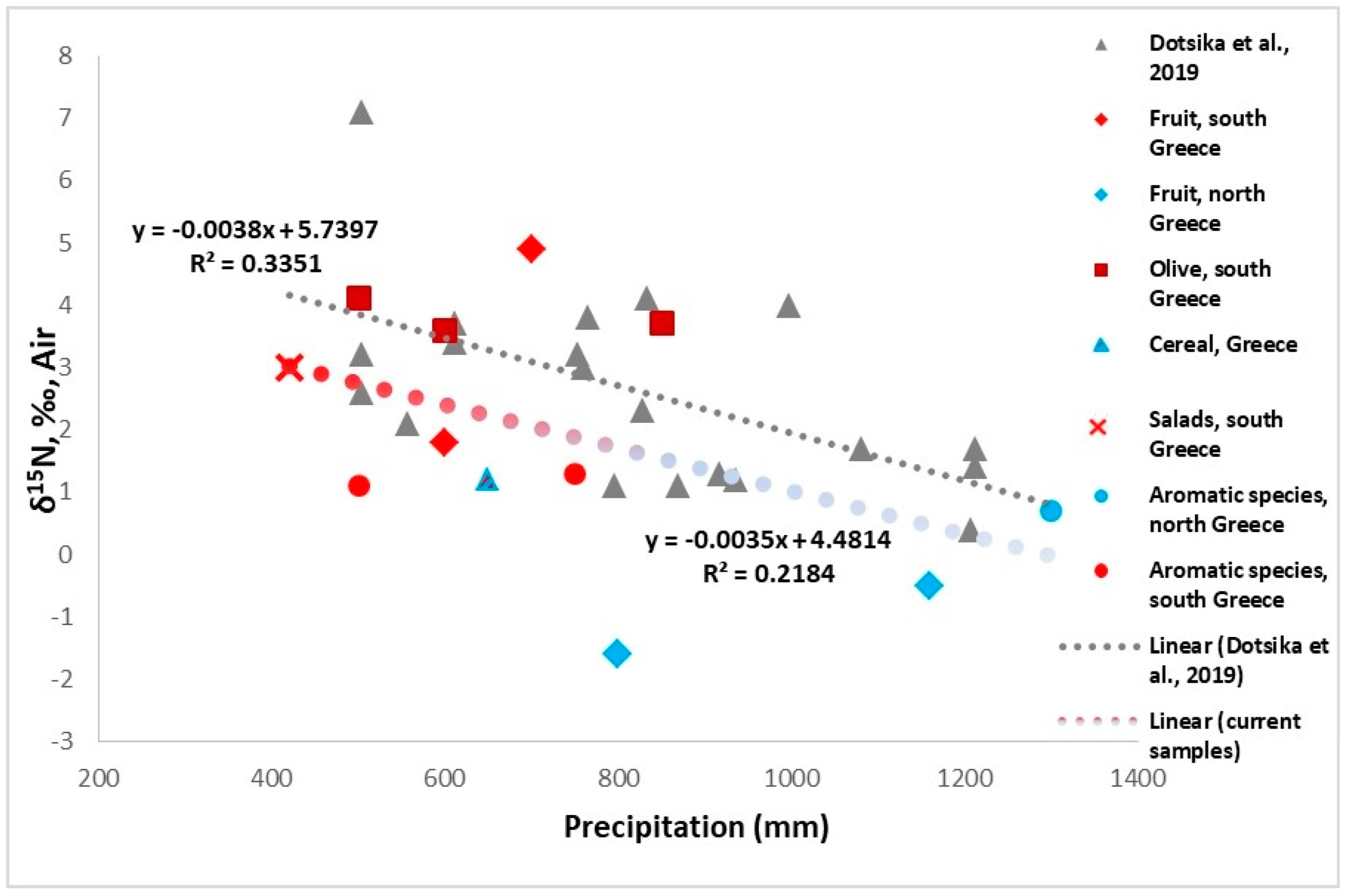
3.1.2. δ15N of Plants

The stable isotope ratio of nitrogen (δ15N) in all the studied plants ranges from -δ 4.0‰ to δ5.1‰ (except for citrus, 12.1‰; see Table 1 and Figure 3 and Figure 4). The observed difference between the samples, approximately δ10‰, cannot be fully explained by the differences in rainfall (Figure 1). It can be attributed to the agricultural regime, climate, altitude, distance from the coast, and different crops. Furthermore, it seems that in some plant species, the high δ15N (>4‰) could be attributed to the proximity to the sea (Ilia region and Sparta area) and/or in arid climates (Nemea area, Sparta area and Heraklion region) since the 15N isotope grows in drought [48,49,50,51,52,53,54,55,56,57,58,59].
In addition, a difference in nitrogen isotope values is observed between northern, central, and southern Greece, most likely indicating that climate significantly impacts the final δ15N values of plants. The nitrogen isotopic values in northern Greece (Kozani and Naousa regions) and central Greece (Fthiotida region) are less than δ2‰, while in Peloponnese (apart from one sample from Messinia of western Peloponnese) and in Crete the nitrogen isotopic values are more than δ2‰ (Figure 3). Dotsika and Diamantopoulos [48] demonstrated that the slope of the variation in δ15N with precipitation is equal to 0.38/100 mm for both Greek plants and herbivores (the calculated slope refers to a range of annual precipitations from 300 to 1200 mm).
The δ15N variation with rain intensity (precipitation) for the plants measured in this work equals 0.48/100 mm (see Figure 5; the data from the Ilia region are not included). This value differs from the previous work [48], possibly due to significant area variations. Even so, it demonstrates a small correlation between nitrogen and climate. The altitude differences between the Olympus Mt. area and the Attika region, as well as between the Olympus Mt. area and Kiato area, could explain the observed discrepancies. In contrast to the altitude differences, the variation in altitude between he Ilia, Messinia, and Fthiotida regions can be attributed to their distance from the coast, the use of fertilizers, and the cultivation of different crops.
The studied plants from the same locality, such as the Messinia, Ilia, and Fthiotida regions and Kiato area, show a difference between each other in nitrogen isotope value of more than δ1-2‰ (Figure 6). This difference is likely due to the use of fertilizers. The same plants from the same area (nearby fields) show different nitrogen isotope values, indicating the use of manuring/fertilization. Different types of fertilizers differentiate the nitrogen isotope [14,57]. Among the studied samples, only one plant showed a noteworthy higher δ15N value (δ12.1‰), which was probably due to the use of animal manure. It is well known that nitrogen in earth is obtained through the use of organic fertilizer inputs. This is explained by the N volatilization during the N mineralization process. The latter enhances heavy nitrogen isotope (δ15N) enrichment in the N sources available for plants, resulting in higher plant δ15N value [62]. In fact, animal manure presents nitrogen values higher than +δ8‰ [63], since animals eat plants (with δ15N values that reflect nitrogen isotopes of soil N (δ4–8‰), except for N-fixing plants, which demonstrate δ15N values similar to those of atmospheric N (δ0‰)), and thus, their wastes show δ15N enrichment due to the fractionation processes (volatilization of ammonia and denitrification or bacterial reworking of N). In contrast, synthetic fertilizers show lower nitrogen values compared to those of organic fertilizers [14,62]. The grains (barley and wheat) exhibit values of 2 ± 1.3‰, demonstrating the use of conventional fertilizers. Busa et al. [60] observed a significant difference between the nitrogen isotopic values for conventionally grown (2.1 ± 0.3‰) and organically grown barley (>3.4 ± 0.5‰) grains. The main reason for this difference is the type of fertilizer used.

3.1.3. δ34S of Plants

The sulfur isotope ratio (δ34S) of the studied plant products (fruits, nuts, cereals, herbal) ranged between −2.1 and 7.3‰ (median δ34S = 2.6‰, sd = 2.2‰; see Table 1). As mentioned above, the primary factors affecting the sulfur isotopes of plants include the soil, the fertilizer, and the atmospheric pollution [8]. The studied plants show δ34S values lower than 7.3‰. However, the geology of Greece is characterized by a highly complex structural system, and it is important to consider that regional soil differences can influence sulfur isotopes. Nevertheless, it can be argued that a standard deviation of more than 2‰ indicates a relatively homogenous sulfur isotope dataset that cannot be attributed solely to soil sulfur. Considering that no significant isotopic fractionation occurs during plant uptake and metabolism [2], probably these plants take the sulfur mainly from the fertilizers [14] and less from the oxidation of mineral soils [2]. The δ34S value of the most common fertilizer is between −10 and 20‰ [2,14].
The lowest δ34S value measured for lentils and tomatoes is −2‰. This value may be attributed to the elevated water uptake by these plants, as they grow in floodplains near river basins [64,65], where δ34S values range from −5‰ to +15‰ [12,13,14,15,16,17,18,19,20]. This cultivating practice can have an important influence on sulfur isotopes due to the geochemical and biological processes occurring in the area’s soil and water. So the lower δ34S value of −2‰ in lentils and tomatoes could indicate that the sulfur available to these plants has a lighter isotopic signature, likely resulting from the elevated water uptake in these areas. The water in floodplains may be enriched with lighter sulfur isotopes, which can be taken up by plants, influencing their δ34S values. This could also reflect biological processes such as sulfate reduction or other microbial activity in the soil, which might preferentially utilize lighter isotopes of sulfur. In this way, the geochemical processes in floodplains, combined with the water uptake by plants, can lead to distinct sulfur isotope signatures in crops like lentils and tomatoes.
The higher measured values of δ34S are >4‰, corresponding to fruits (from Kiato and Sparta areas), nuts, and some cereals. It appears that the type of fertilizers, the aerosol marine, and the soil claim an antagonistic role in the final sulfur value of the products. The potential influence of geological bedrock beneath the soil material in sulfur isotope is difficult to be assessed since the structural geology of Greece is too complex (Figure 7). The wild species from the Olympus Mt. area also present high values of sulfur isotope, depending on local soil sulfur sources and marine aerosol exposure. These terrestrial plants usually show δ34S values in the range from ~+δ 4.2‰, corresponding to inland areas, to ~+δ7.3‰, in the case of coastal regions, due to marine sulfur deposition. The standard deviation of δ1.5‰ is considered an adequately homogenous sulfur isotope dataset of the Olympus Mt. area soil sulfur.
Plants from different areas present distinct patterns of nitrogen and sulfur isotope ratios. Plants from the Naousa region and the Kiato’s coastal areas differ in their δ15N and δ34S, indicating an enrichment in them from the Northern regions towards the Southern ones (Figure 6). The δ15N and the δ34S isotopic data probably suggest that they have been influenced (i) by the climate mainly due to the enrichment of δ15N as a result of relatively low rain accumulation [48], (ii) by the marine aerosol in the case of δ34S dataset, (iii) by the fertilizers and (iv) by the soil reflecting the δ34S dataset (Figure 7). However, taking into account that the plants’ sulfur isotopic values across the country are not really complicated and fluctuated, despite its complex geology (Figure 7), it can thus reasonably be assumed that the “sea-spray effect”, along with rainfall, plays a crucial role in the homogenous range of sulfur isotopic values.

3.1.4. δ13C, δ15N, and δ34S of Marine Species

The fish samples studied come from both marine and freshwater environments. The relatively low carbon values of the marine fish samples state that they might have been caught from waters with significant freshwater influx. In fact, the marine coastal fish samples analyzed in this work include sea bass, groupers, and breams. The δ13C values of these species range from −13.1 to −18.9‰; this value characterizes the species that have been found in shallower waters near shorelines, typically in coastal regions where the depth of the water is less than 200 m. They are often associated with estuaries, bays, and reefs and can tolerate the dynamic conditions of these areas (Euryhaline zone), including changes in salinity, temperature, and depth. Inshore fish, also, such as sparidae (δ13C = −13.1‰ and δ15N = +6.3‰), enter coastal lagoons, estuaries, and salt marshes for spawning. The inshore fishes are commonly found in marine and brackish waters of temperate regions, like those in Greece.
The coastal species found in deeper waters, such as sole and red mullets, present δ13C between −18.3 and −19.5‰, δ15N between 9.6 and 12.7‰, and δ34S values ranging from 17.8 to 18‰. The marine pelagic fish, like mackerels, show δ13C = −17.8‰, δ15N = 10.5‰ and δ34S values = 17‰. Generally, these marine species come from the east coast of the mainland of Greece, and their δ34S values reflect the marine sulfate influence. These coastal species are the most common in archaeological fish assemblages [67,68].
The δ13C values of freshwater fish range from −18.7 to −20.5‰, δ15N values range from 7.5 to 13‰, and δ34S values range from 4.6 to 14‰. These freshwater fish originate from Northern Greece, a region known for its rivers and lakes. Most of these rivers form swamps and lakes before reaching the Aegean coast. This aquatic habitat is also preferred by bream because this fish thrives in slow-moving or still waters and ponds with vegetation- and oxygen-rich conditions. So, the freshwater hydrological system, in Northern Greece, falls largely into the “coastal zone”. The carp and various other cyprinids inhabit these warm, deep, slow-flowing, and still waters (Table 3). For comparison, the δ13C and δ15N values of recent [68] and older [52,69,70,71,72,73] freshwater fish and fauna from the Mediterranean Sea are depicted in Table 4. These findings demonstrate significant similarities between the aforementioned fish samples (see Table 3).

3.2. Isotopic Analysis in Modern Mammals

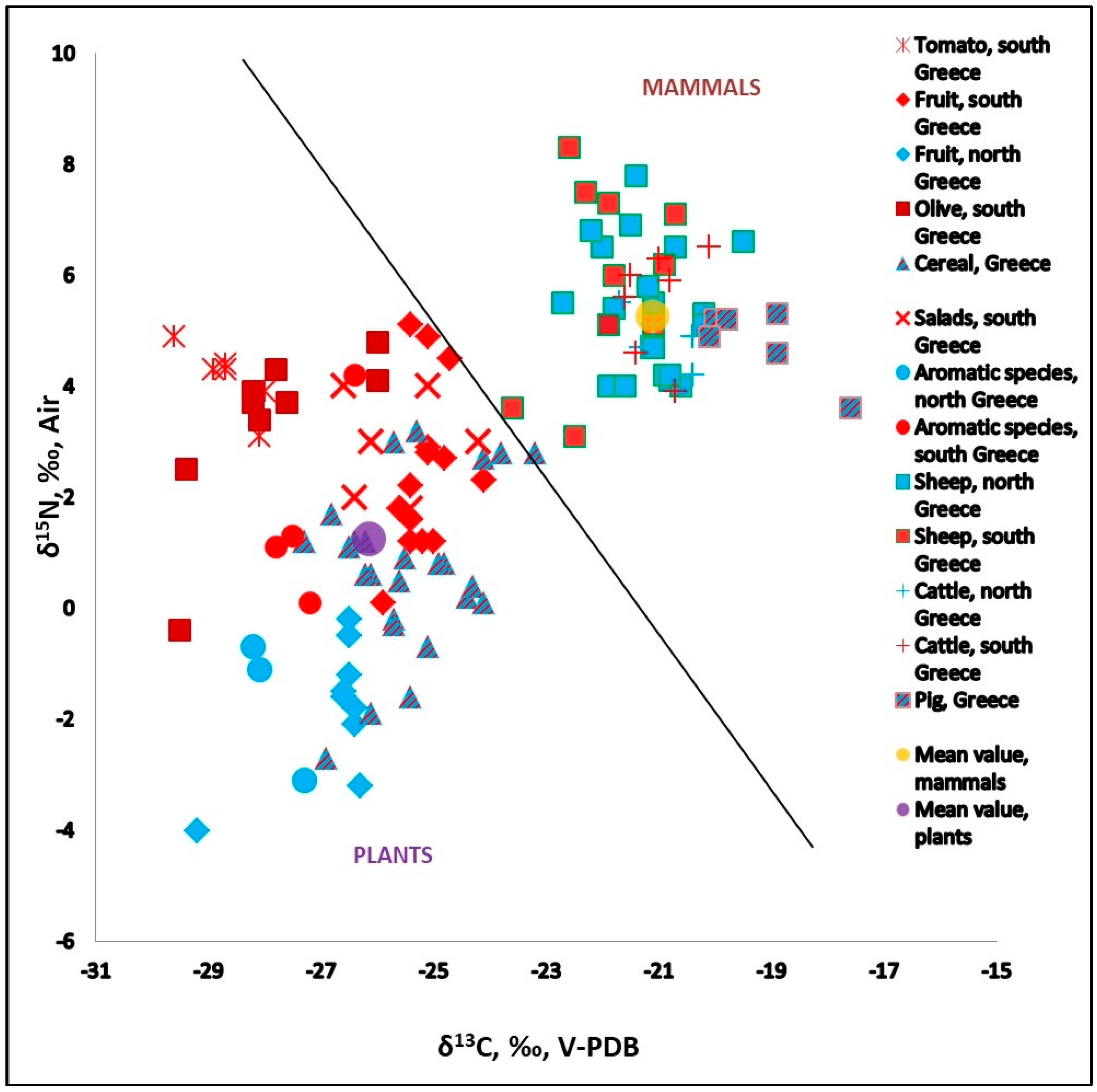
3.2.1. δ13C and δ15N Values of Various Mammals

The δ13C and δ15N values of various herbivores range from −23.6‰ to −19.6‰ and 3.1‰ to 8.3‰, respectively. The δ13C and δ15N values of those mammals from Greece confirm that they consumed a terrestrial C3 plant diet (Figure 8), including traces from a C4 diet (e.g., maize). The difference in carbon isotope values between plants and mammals is attributed to fractionation factors ranging from 1‰ to 5‰ [44,45,74]. In particular, the data indicate an offset for δ13Cco between bone collagen and diet of 5.3‰ (the difference in median between the carbon of plants and collagen values). This range falls into the offset, from 1‰ to 5‰ mentioned in previous studies [46,75,76]. Also, a statistical study conducted by Fernandes et al. [77] determined an offset at 4.8‰ for carbon collagen isotope with an uncertainty at 0.5‰. The statistical study of Fernandes et al. [77] assessed isotopic data collected by Froehle et al. [78] of measurements performed on omnivorous mammals during controlled feeding experiments [44,45,75,76,79].

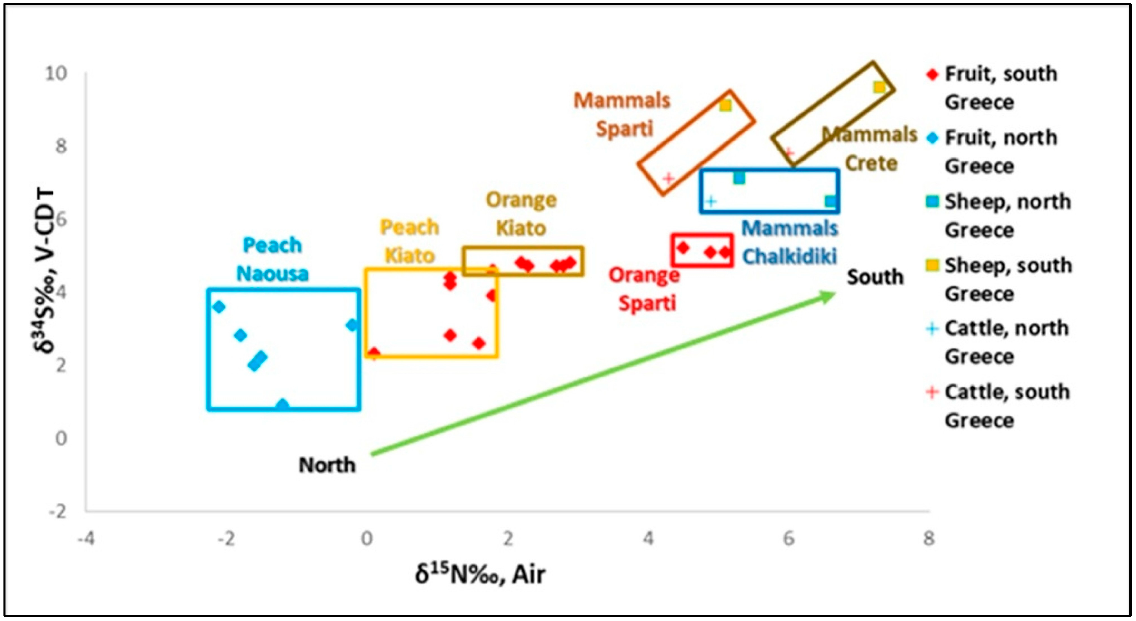
3.2.2. δ34S Values of Various Mammals

The δ34S values of various herbivores range between 4.0‰ and 9.7‰. Taking into account that the isotope fractionation between the dietary sulfate and the bone collagen averages 1‰ [21,34,35], the difference in δ34S values observed between the diet and the mammals’ collagen (more than 5‰) indicates that these mammals obtained their food from different geographical areas (Table 5). However, the animals (cattle) from the same area (Chalkidiki peninsula) demonstrate a difference in sulfur isotopes greater than 1‰, which is probably due to sulfide ore deposits. Herbivores primarily feed on grass, which constitutes the bulk of their diet. Fresh grass absorbs sulfur from the soil and atmosphere during growth. This sulfur can originate from natural sources or anthropogenic sources. Therefore, herbivores from the same area should present the same sulfur isotope, although herbivores from the entire Greek region should provide an sd > 2‰, especially because of the complex geology of Greece. Similarly to sulfur isotopic values in plants, the δ34S values in mammals demonstrate regional soil differences that can influence sulfur isotopes, which were not recorded in isotopic data. Sulfur isotopic values in Greek herbivorous mammals reflect a homogenous sulfur isotope dataset that could not be related to soil sulfur. In particular, animals (cattle, free-range) from the same area (Chalkidiki), present a difference in sulfur isotopes greater than 1‰ (sd = 1.8‰), which is probably due to different soil elements.
The local flora from the Chalkidiki peninsula can take up sulfur from atmospheric reservoirs, freshwater (δ34S values range between 21.4 and 10.1‰ [82]), thermal water (δ34S values range between 12.6 and 13.8‰) [78] and mainly sulfide minerals. It is well known that the Chalkidiki peninsula hosts enormous massive sulfide ore deposits and, thus, is a metalliferous area (e.g., [83,84,85]). The pyrite presents δ34S values ranging from −1 to 3‰. Therefore, the δ34S value of sulfur in Chalkidiki could range from −1 to +21.4‰. Considering the fractionation factors, plants are depleted in δ34S by −1 to −2‰ relative to their S source, and vegetation in Chalkidiki could show δ34S values between −3 and +20‰. In addition, considering that mammals are not fractionated in their diet [35,86], domestic animals raised in Chalkidiki that consume local vegetation could not present δ34S values greater than 20‰. Mammals from Chalkidiki have a δ34S value of less than 20‰. So, lower sulfur isotope values probably mean that the animals grazed on vegetation that obtains its sulfur mainly from δ34S-depleted minerals. On the other hand, δ34S values likely indicate that the animals grazed closer to δ34S-enriched geothermal water sources or grazed on coastal vegetation affected by sea spray, as in the present study. Furthermore, a difference between nitrogen and sulfur isotope values was also observed, which may also be explained by different husbandry methods and by climate: animals from the same area [i.e., Chalkidiki, standard deviation (cattle), δ34S, 1.8‰] present distinct patterns in nitrogen and sulfur isotope ratios.
The distribution of mammals from various regions of Greece is reported herein (Figure 9). Regardless of the origin, it has been observed that cattle present lower δ34S values compared to those values of lambs. Moreover, mammals (cattle and sheep) from the Chalkidiki peninsula and Crete Island differ in their δ15N and δ34S values by more than 1‰ (see Figure 9). The concurrent difference in these isotopes suggests divergence in the day-to-day raising methodology applied in animal husbandry (such as care production, nutrition, breeding, mobility, or grazing on different lands). This disparity in livestock practices is supported by the distinct sulfur isotopic values found in the various environments. In theory, there should be differences in the δ34S values of animals feeding predominantly on resources coming from different geological areas (e.g., plains near the city or mountains or resources coming from other countries).
However, the above analysis model is not valid when Chalkidiki is compared to the Sparta area: elevated sulfur isotopic values are observed from North to South while nitrogen values are reduced (Figure 9). Furthermore, sulfur enrichment between the north and south is observed, even when we compare plants and mammals (Figure 10). Nevertheless, the mammals that originate from the Sparta area always demonstrate an increase in sulfur isotopic values following a decrease in nitrogen values from north to south. According to Dotsika and Diamantopoulos [48], rainfall affects nitrogen isotopic values (the slope of the variation in δ15N with precipitation is equal to 0.38/100 mm for both Greek plants and herbivores). The isotopic results show that the lower nitrogen isotopic values in Sparta compared to those in Chalkidiki are due to higher rainfall in the former. The average rainfall at the A. Dimitriou and Elos stations (Sparta area) over the last 22 years was 650 mm and 505 mm, respectively. On the other hand, the average rainfall at the A. Prodromos and Arnaia stations (Chalkidiki peninsula) over the last 35 years was 420 mm and 440 mm, respectvely (Impact Investigation of variable rainfall in areas of the Greek territory, NTUA [87]). This indicates that the climate (rainfall) affects the values of the isotopes.
The average sulfur levels in pigs are higher than those in herbivores, which can be attributed to their omnivorous diets. However, the δ15N values of pigs (Table 2) do not align with those typically associated with a mixed diet [88]. Weber et al. [88] demonstrated a strong linear relationship between δ15N values in all tissues and the amount of marine protein consumed. When (at least) 25% of the dietary protein has a marine origin, then the δ15N values start to increase consistently among individuals consuming the same diet [89]. Additionally, adolescent pigs consistently showed lower δ15N values compared to piglets or sows consuming the same diet [88]. The observed high carbon values indicate minimal contributions from C4 plants in their diet (Table 2). In conclusion, higher δ34S values may indicate a small proportion of marine protein, such as fishmeal, in the diet or could result in the consumption of vegetation enriched in marine-derived sulfur. This suggests, in this case, that the studied pigs likely grew up closer to the coast.

4. Sulfur Isotope Analysis in Modern Terrestrial, Marine, and Freshwater Environments: Contribution of the Paleo Diet and Paleo Mobility Studies

In order to assess the paleo diet reconstruction, δ13C, δ15N, and δ34S isotopic values have been plotted (see Figure 11 and Figure 12), along with relevant conversions used in this (paleo) diet study (Table 6), illustrating the modern terrestrial, freshwater, and marine reservoirs, as derived from this research. It is noteworthy to mention herein that the findings are constrained by either a lack of sample size or a lack of samples from various locations, while all modern carbon isotopic values are calibrated to ancient ones [90] in order to compare them with available archaeological data. In fact, the geological complexity of Greece can lead to variations in isotopic signatures due to differences in local rock composition, soil chemistry, and water sources. These variations can make it difficult to establish clear baselines for ecological and nutritional reconstructions. However, to mitigate these challenges, we used multi-isotopic approaches, including carbon, nitrogen, and sulfur and compared the results with the data of archaeological specimens (Table 5). Furthermore, because the comparison between modern and ancient samples may overlook temporal changes in dietary practices and environmental conditions, potentially leading to misinterpretations of ancient diets, we compared modern samples and samples from archaeological and historical contexts with known environmental and dietary characteristics [68,69,70].
Findings document that all the fish species analyzed here are carnivores that consume herbivorous fish, crustaceans, and mollusks. The results show that recent marine fish, as a dietary resource, exhibit variable isotopic compositions, i.e., a total range of 6.4‰ for δ13C, 7.1‰ for δ15N and 4.7‰ for δ34S. The observed range of δ15N values indicates that the studied fish species live at different trophic levels, with the grouper existing at the highest level (each successive step in the food chain corresponds to an increase of about 3‰ in δ15N values, [46]). In principle, the increase in δ15N content during assimilation from one trophic level to another depends on the number of steps in the food web.
Moreover, the modern results were compared to the bibliographical data referring to the δ13C and δ15N of fish bones’ values from the archaeological sites (Table 4) [69,71]. Even if a correlation between the recent and the ancient fish species leads to the conclusion that both groups fall into the same range, a detailed comparison of each species emphasizes significant isotopic differences between them. The recent Sparidae specimen shows the highest δ13C values, −13.1‰ (δ15N = 6.3‰, δ34S = 18.5‰), whereas the recent Scombridae specimen exhibits the lowest δ13C values, −17.8‰ (δ15N = 10.5‰, δ34S = 17‰). The maximum difference between recent and old fish from the same specimen (Sparidae) is 0.5‰ for δ13C values and 3‰ for δ15N (not available data for δ34S), while for the Scombridae specimens, it is 3.3‰, for δ13C values and 1.5‰ for δ15N. In general, there are more significant differences between ancient individuals from the same species, e.g., for sparidae (median δ13C = −12.6‰, sd:3.7‰) and Scombridae (median δ13C = −14.4‰, sd:2.1‰), than between recent individuals from different species (median δ13C = −16.3‰, sd:2.3‰). Furthermore, in freshwater fish species, there are differences between ancient (median δ13C = −19.2‰, sd: 3.1‰; δ15N = 8.7‰, sd:1.3‰) and recent individuals (Cyprinidae) (median δ13C = −17.9‰, sd:0.9‰; δ15N = 8.0‰, sd: 3.0‰). The differences between marine and freshwater fish species are either due to the diversity in the trophic structure of marine ecosystems, probably reflecting the natural changes in local environmental conditions or even due to modern human activities (e.g., fishing, overfishing, aquaculture, or contamination). All these aspects can be considered as potential factors affecting the great range of the obtained isotopic results, which in turn reflect the changes in trophic structures and feeding strategies and, particularly, the feeding strategies adopted by various fish species.
The fish species living at low levels exhibit δ13C and δ15N values very close to those of terrestrial resources (see Figure 11 and Figure 12), which means that it is difficult to detect them isotopically. This indicates that it is difficult to detect a fish consumption of less than 10% of the total diet by weight, and so, the isotopic values of human collagen would be closer to a C3 terrestrial diet. Furthermore, zooarchaeological data (see Table 5) have been incorporated into Figure 11 and Figure 12. They concern stable sulfur isotope analysis from Greek remains: (a) the analysis of assemblages from the Bronze Age sites at Chamalevri (mammal samples, 13 Km from Rethymno) in Crete [48] and (b) the analysis of assemblages from Thessaly, central Greece, dating to the Early Iron Age [72] and the local archaeofauna (mainly ovicaprids) from the Classical site of Thebes (5th c. BC) [73]. Animal δ34S values range from 2 to 18.2‰ [51,72,73]. The data from Crete and Thebes [52,73] have shown that coastal sites, while having a terrestrial diet based on C-N isotopic values, show high δ34S values closer to marine values (≈+20‰) due to the sea spray effect. In contrast, the δ34S values of the mammals from Thessaly (Voulokaliva and Kephalosi coastal sites) have not been influenced by the “sea-spray” like in the case studies of Crete and Thebes [51,73].
At the same time, a comparison between recent and ancient mammals demonstrates that both groups drop in the same range. Nevertheless, minor isotopic differences among them might be attributed to intensive exploitation and the systematic cultivation of faunal (different fodder) and flora (cereals and legumes). On the other hand, there are major δ34S differences (Table 5) among ancient and recent herbivore individuals rather than between recent mammals of different species. The low standard deviation (SD: 1.47‰; see Table 5) of recent herbivores mammals reflects a homogenous sulfur isotope data set. This could be attributed to the regional differences caused by the complex structural geology of Greece (see Figure 7) and therefore is depicted in sulfur isotopes. The larger isotope sulfur differences between ancient and recent cattle from Crete Island are probably caused by the diversity in the trophic structure of terrestrial ecosystems and may reflect the natural changes in local environmental conditions or modern human activities. Considering the geological structure of Crete, higher values of sulfur isotopes would be expected, particularly in the central and the southern parts of the Island, where Richards et al. [81] analyzed archaeological faunal bones from Apodoulou (South Crete, Middle Minoan period). In these areas, the Messinian evaporites are more prevalent and have a wider geographical distribution. These evaporitic formations were deposited during the Messinian Salinity Crisis (MSC), which resulted in the extensive formation of evaporitic deposits throughout the Mediterranean Sea [89,91]. In other parts of Crete, such as the western provinces of Chania and Rethymno, evaporites are relatively rare. Instead, they are replaced by other deposits relevant to desiccation, such as shallow water carbonates, partly travertine- and microbial-mat-type deposits, and Lago Mare [91]. Therefore, in these areas, lower sulfur values are expected. However, contrary to what is observed, higher sulfur isotopic values are detected in Chamalevri (δ34S of sheep range from 12.6 to 13.5‰) compared to Apodoulou (δ34S of sheep range from 10.0 to 10.9‰) according to Richards et al. [81]. It appears that sulfur derived from the geological substrate (evaporite minerals) in the soil was not sufficient to outweigh the contributions of marine aerosols and rainfall. The closer proximity to the sea and the lower altitude of Chamalevri (80 m, 13 km from Rethymno) make it more susceptible to the influence of marine aerosols, which—in other words—may contribute to elevated sulfur values. In contrast, Apodoulou (430 m, 54 km from Rethymno), being further inland and at a higher elevation, experiences a reduced impact from marine aerosols. This suggests a competitive role of marine aerosols in relation to soil sulfur contributions in the distribution of sulfur at these locations.
In conclusion, a major problem with sulfur isotopic values is the degree of overlap between freshwater and terrestrial species. It appears that locations with complex surface geology, geography and topography, like Greece, produce a diverse terrestrial δ34S composition, which is reflected in terrestrial floral and faunal δ34S. Such diverse terrestrial δ34S values result in difficult discrimination between freshwater and terrestrial species. Nevertheless, until now, sulfur isotopic values of recent plants, mammals, and fishes, which could potentially help in the paleo diet, paleomobility, and paleoecology reconstruction, had been lacking from Greece.
The sulfur isotope is an important tool because it has the potential:
(a) To refine palaeodietary profiles by lending support to conclusions based upon δ13C and δ15N;
(b) To identify better the participation of marine protein in diets;
(c) To distinguish between freshwater and terrestrial dietary sources, enabling better recognition of the paleo diet human profile;
(d) To exclude potential foods with very different δ34S relative to those of humans;
(e) To provide information about human mobility and migration because the sulfur values are connected with the geological background of a geographical region;
(f) To detect other factors (such as regional soil differences, salinity, and aerosol) that can influence sulfur isotopes;
(g) To recognize agricultural practices (intensive exploitation and systematic cultivation) and the anthopogenetic factors (atmospheric pollution) that influence sulfur isotopes (such as atmospheric pollution);
(h) To trace animal husbandry (sulfur isotope values provide evidence of the impact of husbandry methods) practices (such as care production, nutrition, breeding, potential mobility, or grazing on different lands).
Sulfur isotopic analysis also has the potential to differentiate between local animals and those imported from or raised in other locations. Isotope analysis promises to be a useful addition to support archaeometric studies (palaeodietary, paleomobility, and migration examination).
It should be pointed out that the comparison between modern and ancient samples may not fully account for long-term environmental changes. Certainly, the cumulative effects of land use changes (urbanization, deforestation, agricultural expansion, changes in land management, and climate shifts) and other anthropogenic impacts (infrastructure and industry, biodiversity loss, ecosystem disintegration, desertification, increased CO2 emissions, changes in the hydrological cycle, population movements, and changes in the agricultural economy) could alter baseline isotopic signatures over time.
All the conversions used in this study are illustrated in Table 6. In order to compare modern carbon isotopic values with archaeological data, all the values have been calibrated to ancient ones [90].
Table 6. Values for converting data to Modern Hair Keratin (MKE) and to Modern Diet Equivalent (MDE). * δ34S values of fractions from pig tissues under a Controlled Diet [36]; ** δ34S values of fractions from ox and goat tissues under a Controlled Diet [19]; *** δ34S values of fractions from horses under a Controlled Diet (C3—plant diet; C4—plant diet).
Conversion Data to Modern Hair Keratin (MKE) and to Modern Diet Equivalent (MDE)δ13C (‰)
‰, V-PDB
δ15N (‰)
‰, V-AIR
δ34S
‰, V-CDT
Source
Convert modern bone collagen to modern (2010) hair keratin (MKE)−1.4−0.9 [51]
Convert ancient atmospheric δ13C to modern (2010) atmospheric equivalent δ13C−1.9- [90]
Convert ancient bone collagen to Modern Hair Keratin (MKE), including conversion to modern CO2, δ13C−3.3−0.9 [92]
Convert modern keratin equivalent (MKE) to Modern Diet Equivalent (MDE)−2.5−5.15 [50,51]
Convert modern bone collagen to modern hair keratin (MKE) +2.5 *
+0.4 to +4.0 **
* [34]
** [8]
Convert modern bone collagen to Modern Diet Equivalent (MDE) +1.5 *
−0.5 to +0.5 **
* [34]
** [8]
Convert modern keratin to Modern Diet Equivalent (MDE) −2 *
−5 to −2 **
+1 (C3-plant diet) to
– 4 (C4-plant diet) ***
* [34]
** [8]
*** [35]

5. Conclusions

This study presents an extensive and thorough collection of sulfur isotope values from modern samples originating from Greece. The samples include C3 and C4 plants, terrestrial animals (mammals), and aquatic life, i.e., fish. An analytical approach of the sulfur isotope values, along with carbon and nitrogen isotopes, provides valuable insights into the human diet, mobility, and residence for forensic studies.
The δ34S, δ13C, and δ15N analysis of various plants and animals from Greece revealed a clear imprint in δ34S values demonstrating differences between terrestrial and aquatic animals derived from dietary resources from marine and/or freshwater reservoirs. The sulfur isotopic values of plants suggest that they have been mainly influenced by the rainfall, the marine aerosol, and the type of fertilizers used. Despite the fact that the geological structure of Greece is rather complex, the results yielded were not expected, suggesting that geology affected sulfur values much less than other factors.
While variations in the δ34S values of animals that are fed mainly with resources originating from different geological regions (e.g., plains near cities or close to mountains, imported resources from other countries) might be expected, the results of the study do not prove this hypothesis. Thus, it can be assumed that the “sea spray effect” and rainfall both play a crucial role in the homogeneous range of sulfur isotopic values in Greece. Additionally, even if the data at first glance indicate that the regional geological setting plays an important role in the sulfur isotope fingerprinting, it appears to corroborate that the type of fertilizers, the aerosol marine, and the soil claim an antagonistic role in the final sulfur value of the products. Furthermore, the observed substantial overlaps reduce the effect of the application of sulfur to palaeodietary reconstruction. In various localities with a uniform surface geology, negligible variation in the geological source(s) of sulfur is observed, which is ultimately assimilated by terrestrial fauna. On the other hand, freshwater fish present more diverse sulfur sources in contrast to terrestrial fauna in areas with complicated surface geology, as the former exhibit different and variable δ34S profiles compared to the latter.
To the best of our knowledge, the sulfur isotopic dataset values of recent plants, mammals, and fish from Greece presented herein comprise a novel approach for the first time in the literature. It is an attempt to fill the knowledge gap, allowing a better understanding of the factors that influence the imprint of sulfur isotopes and, moreover, to give an understanding of a paleo diet, paleomobility, and paleoecology reconstruction.

Author Contributions

Conceptualization, E.D. and P.K.; methodology, A.-E.P.; software, G.D.; validation, L.G., S.B. and D.K.; formal analysis, D.K.; investigation, E.D.; resources, A.-E.P.; data curation, P.N.G.; writing—original draft preparation, P.K.; writing—review and editing, D.K.; visualization, E.D.; supervision, E.D.; project administration, E.D.; funding acquisition, P.K. All authors have read and agreed to the published version of the manuscript.

Funding

This research received no external funding.

Informed Consent Statement

No ethical issues are derived from this research since it is unrelated to animal testing.

Data Availability Statement

The data presented in this work are produced within analytical experiments at the Stable Isotope Unit in the National Centre of Scientific Research. All data generated or analyzed during this study are included in this published article.

Conflicts of Interest

The authors declare no conflicts of interest.

References

  1. Cernusak, L.A.; Ubierna, N.; Winter, K.; Holtum, J.A.M.; Marshall, J.D.; Farquhar, G.D. Environmental and physiological determinants of carbon isotope discrimination in terrestrial plants. New Phytol. 2013, 200, 950–965. [Google Scholar] [CrossRef] [PubMed]
  2. Tcherkez, G.; Tea, I. 32S/34S isotope fractionation in plant sulphur metabolism. New Phytol. 2013, 200, 44–53. [Google Scholar] [CrossRef]
  3. Chung, I.M.; Lee, T.J.; Oh, Y.-T.; Ghimire, B.K.; Jang, I.B.; Kim, S.H. Ginseng authenticity testing by measuring carbon, nitrogen, and sulfur stable isotope compositions that differ based on cultivation land and organic fertilizer type. J. Ginseng Res. 2017, 41, 195–200. [Google Scholar] [CrossRef] [PubMed]
  4. Evans, R.D. Physiological mechanisms influencing plant nitrogen isotope composition. Trends Plant Sci. 2001, 6, 121–126. [Google Scholar] [CrossRef]
  5. Barbour, M.M. Stable oxygen isotope composition of plant tissue: A review. Plant Biol. 2007, 34, 83–94. [Google Scholar] [CrossRef] [PubMed]
  6. Giannioti, Z.; Ogrinc, N.; Suman, M.; Camin, F.; Bontempo, L. Isotope ratio mass spectrometry (IRMS) methods for distinguishing organic from conventional food products: A review. TrAC Trends Anal. Chem. 2024, 170, 117476. [Google Scholar] [CrossRef]
  7. Trust, B.A.; Fry, B. Stable sulphur isotopes in plants: A review. Plant Cell Environ. 1992, 15, 1105–1110. [Google Scholar] [CrossRef]
  8. Tanz, N.; Schmidt, H.-L. δ34S-Value Measurements in Food Origin Assignments and Sulfur Isotope Fractionations in Plants and Animals. J. Agric. Food Chem. 2010, 58, 3139–3146. [Google Scholar] [CrossRef]
  9. Chalk, C.P.; Inácio, C.T.; Chen, D. Tracing S dynamics in agro-ecosystems using 34S. Soil Biol. Biochem. 2017, 114, 295–308. [Google Scholar] [CrossRef]
  10. Claypool, G.E.; Holser, W.T.; Kaplan, I.R.; Sakai, H.; Zak, I. The age curves of sulfur and oxygen isotopes in marine sulfate and their mutual interpretation. Chem. Geol. 1980, 28, 199–260. [Google Scholar] [CrossRef]
  11. Krouse, H.R.; Mayer, B. Sulphur and Oxygen Isotopes in Sulphate. In Environmental Tracers in Subsurface Hydrology; Cook, P.G., Herczeg, A.L., Eds.; Springer: Boston, MA, USA, 2000; pp. 195–231. [Google Scholar] [CrossRef]
  12. Hoefs, J. Stable Isotope Geochemistry; Springer: Berlin/Heidelberg, Germany, 2006. [Google Scholar]
  13. Nielsen, H.; Pilot, J.; Grinenko, L.N.; Grinenko, V.A.; Lein, A.Y.; Smith, J.W.; Pankina, R.G. Lithospheric Sources of Sulphur. In Stable Isotopes: Natural and Anthropogenic Sulphur in the Environment; Krouse, H.R., Grinenko, V.A., Eds.; Wiley: Hoboken, NJ, USA, 1991; pp. 65–132. [Google Scholar]
  14. Vitòria, L.; Otero, N.; Soler, A.; Canals, À. Fertilizer Characterization: Isotopic Data (N, S, O, C, and Sr). Environ. Sci. Technol. 2004, 38, 3254–3262. [Google Scholar] [CrossRef]
  15. Ault, W.U.; Kulp, J.L. Isotopic geochemistry of sulphur. Geochim. Cosm. Act. 1959, 16, 201–235. [Google Scholar] [CrossRef]
  16. Thode, H.G.; Monster, J.; Dunford, H.B. Sulphur isotope geochemistry. Geochim. Cosmochim. Acta 1961, 25, 159174. [Google Scholar] [CrossRef]
  17. Rees, M.C.; Minson, D.J. Fertilizer sulphur as a factor affecting voluntary intake, digestibility and retention time of pangola grass (Digitaria decumbens) by sheep. Br. J. Nutr. 1978, 39, 5–11. [Google Scholar] [CrossRef]
  18. Böttcher, F.; Barth, S.; Peinke, J. Small and large scale fluctuations in atmospheric wind speeds. Stoch. Environ. Res. Risk Assess. 2007, 21, 299–308. [Google Scholar] [CrossRef]
  19. Nriagu, J.O.; Coker, R.D.; Barrie, L.A. Origin of sulphur in Canadian Arctic haze from isotope measurements. Nature 1991, 349, 142–145. [Google Scholar] [CrossRef]
  20. Baryakhtar, I.V.; Ivanov, B.A. Vector field dynamic. Phys. Lett. A 1983, 98, 222–226. [Google Scholar] [CrossRef]
  21. Nehlich, O. The application of sulphur isotope analyses in archaeological research: A review. Earth-Sci. Rev. 2015, 142, 1–17. [Google Scholar] [CrossRef]
  22. Deegan, L.; Garritt, R. Evidence for spatial variability in estuarine food webs. Mar. Ecol. Prog. Ser. 1997, 147, 31–47. [Google Scholar] [CrossRef]
  23. Leakey, C.D.; Attrill, M.J.; Jennings, S.; Fitzsimons, M.F. Stable isotopes in juvenile marine fishes and their invertebrate prey from the Thames Estuary, UK, and adjacent coastal regions. Estuar. Coast. Shelf Sci. 2008, 77, 513–522. [Google Scholar] [CrossRef]
  24. Fry, B. Stable Isotope Ecology; Springer: New York, NY, USA, 2006. [Google Scholar]
  25. Amrani, A.; Said-Ahmad, W.; Shaked, Y.; Kiene, R.P. Sulfur isotope homogeneity of oceanic DMSP and DMS. Earth Atmos. Planet. Sci. 2013, 110, 18413–18418. [Google Scholar] [CrossRef] [PubMed]
  26. Thode, H.G. Sulphur isotopes in nature and the environment: An overview. In Stable Isotopes: Natural and Anthropogenic Sulphur in the Environment; Krouse, H.R., Grinenko, V.A., Eds.; Wiley: Hoboken, NJ, USA, 1991. [Google Scholar]
  27. Bataille, C.P.; Jaouen, K.; Milano, S.; Trost, M.; Steinbrenner, S.; Crubézy, É.; Colleter, R. Triple sulfur-oxygen-strontium isotopes probabilistic geographic assignment of archaeological remains using a novel sulfur isoscape of western Europe. PLoS ONE 2021, 16, e0250383. [Google Scholar] [CrossRef]
  28. Mahowald, N.M.; Muhs, D.R.; Levis, S.; Rasch, P.J.; Yoshioka, M.; Zender, C.S.; Luo, C. Change in atmospheric mineral aerosols in response to climate: Last glacial period, preindustrial, modern, and doubled carbon dioxide climates. J. Geophys. Res. Atmos. 2006, 111. [Google Scholar] [CrossRef]
  29. Drake, N.A.; Eckardt, F.D.; White, K.H. Sources of sulphur in gypsiferous sediments and crusts and pathways of gypsum redistribution in southern Tunisia. Earth Surf. Process. Landf. 2004, 29, 1459–1471. [Google Scholar] [CrossRef]
  30. Bocherens, H.; Drucker, D.G.; Taubald, H. Preservation of bone collagen sulphur isotopic compositions in an early Holocene river-bank archaeological site. Palaeogeogr. Palaeoclim. Palaeoecol. 2011, 310, 32–38. [Google Scholar] [CrossRef]
  31. Nehlich, O.; Fuller, B.T.; Jay, M.; Mora, A.; Nicholson, R.A.; Smith, C.I.; Richards, M.P. Application of sulphur isotope ratios to examine weaning patterns and freshwater fish consumption in Roman Oxfordshire, UK. Geochim. Cosmochim. Acta 2011, 75, 4963–4977. [Google Scholar] [CrossRef]
  32. Drucker, D.G.; Valentin, F.; Thevenet, C.; Mordant, D.; Cottiaux, R.; Delsate, D.; Van Neer, W. Aquatic resources in human diet in the Late Mesolithic in Northern France and Luxembourg: Insights from carbon, nitrogen and sulphur isotope ratios. Archaeol. Anthr. Sci. 2018, 10, 351–368. [Google Scholar] [CrossRef]
  33. Rodiouchkina, K.; Rodushkin, I.; Goderis, S.; Vanhaecke, F. A comprehensive evaluation of sulfur isotopic analysis (δ34S and δ33S) using multi-collector ICP-MS with characterization of reference materials of geological and biological origin. Anal. Chim. Acta 2022, 1240, 340744. [Google Scholar] [CrossRef]
  34. Webb, E.C.; Lewis, J.; Shain, A.; Kastrisianaki-Guyton, E.; Honch, N.V.; Stewart, A.; Miller, B.; Tarlton, J.; Evershed, R.P. The influence of varying proportions of terrestrial and marine dietary protein on the stable carbon-isotope compositions of pig tissues from a controlled feeding experiment. Sci. Technol. Archaeol. Res. 2017, 3, 28–44. [Google Scholar] [CrossRef]
  35. Richards, M.P.; Fuller, B.T.; Sponheimer, M.; Robinson, T.; Ayliffe, L. Sulphur isotopes in palaeodietary studies: A review and results from a controlled feeding experiment. Int. J. Osteoarchaeol. 2003, 13, 37–45. [Google Scholar] [CrossRef]
  36. Ehleringer, J.R. Interpreting Stable Isotope Ratios in Plants and Plant-Based Foods. Ιn Food Forensics; Carter, J.F., Chesson, L.A., Eds.; CRC Press: Boca Raton, FL, USA, 2017; pp. 46–62. [Google Scholar]
  37. Farquhar, G.D.; Ehleringer, J.R.; Hubick, K.T. Carbon Isotope Discrimination and Photosynthesis. Annu. Rev. Plant Biol. 1989, 40, 503–537. [Google Scholar] [CrossRef]
  38. Smith, B.N.; Epstein, S. Two categories of 13C/12C ratios for higher plants. Plant Physiol. 1971, 47, 380–384. [Google Scholar] [CrossRef]
  39. Walker, P.L.; Deniro, M.J. Stable nitrogen and carbon isotope ratios in bone collagen as indices of prehistoric dietary dependence on marine and terrestrial resources in Southern California. Am. J. Phys. Anthr. 1986, 71, 51–61. [Google Scholar] [CrossRef] [PubMed]
  40. Richards, M.P.; Schulting, R.J. Touch not the fish: The Mesolithic-Neolithic change of diet and its significance. Antiquity 2006, 80, 444–456. [Google Scholar] [CrossRef]
  41. Krueger, H.W.; Sullivan, C.H. Models for carbon isotope fractionation between diet and bone. In Stable Isotopes in Nutrition; Turnlund, J.R., Johnson, P.E., Eds.; ACS Symposium Series: Washington, DC, USA, 1984; Volume 258, pp. 205–220. [Google Scholar]
  42. Lee-Thorp, J.A. On isotopes and old bones. Archaeometry 2008, 50, 925–950. [Google Scholar] [CrossRef]
  43. Ambrose, S.H.; Norr, L. Experimental evidence for the relationship of the carbon isotope ratios of whole diet and dietary protein to those of bone collagen and carbonate. In Prehistoric Human Bone: Archaeology at The Molecular Level; Lambert, J., Grupe, G., Eds.; Springer: Berlin/Heidelberg, Germany, 1993; pp. 1–37. [Google Scholar]
  44. Ambrose, S.H. Preparation and characterization of bone and tooth collagen for isotopic analysis. J. Archaeol. Sci. 1990, 17, 431–451. [Google Scholar] [CrossRef]
  45. Tieszen, L.; Fagre, T. Effect of Diet Quality and Composition on the Isotopic Composition of Respiratory CO2, Bone Collagen, Bioapatite, and Soft Tissues. In Prehistoric Human Bone; Lambert, J., Grupe, G., Eds.; Springer Nature: Dordrecht, The Netherlands, 1993; pp. 157–171. [Google Scholar] [CrossRef]
  46. Fernández, R.D.; Arenas, R. The Late Devonian Variscan suture of the Iberian Massif: A correlation of high-pressure belts in NW and SW Iberia. Tectonophysics 2015, 654, 96–100. [Google Scholar] [CrossRef]
  47. Chartrand, M.; Gilles, S.-J. Forensic Attribution of CBRNE Materials: (A Chemical Fingerprint Database 2015); Government of Canada: Ottawa, ON, Canada, 2015; Available online: http://cradpdf.drdc-rddc.gc.ca/PDFS/unc200/p801299_A1b.pdf (accessed on 12 May 2024).
  48. Dotsika, E.; Diamantopoulos, G. Influence of Climate on Stable Nitrogen Isotopic Values of Contemporary Greek Samples: Implications for Isotopic Studies of Human Remains from Neolithic to Late Bronze Age Greece. Geosciences 2019, 9, 217. [Google Scholar] [CrossRef]
  49. Heaton, T.H.E. The 15N/14N ratios of plants in South Africa and Namibia: Relationship to climate and coastal/saline environments. Oecologia 1987, 74, 236–246. [Google Scholar] [CrossRef]
  50. O’Connell, T.C.; Hedges, R.E. Investigations into the effect of diet on modern human hair isotopic values. Am. J. Phys. Anthr. 1999, 108, 409–425. [Google Scholar] [CrossRef]
  51. O’Connell, T.C.; Hedges, R.E.M.; Healey, M.A.; Simpson, A.H.R.W. Isotopic Comparison of Hair, Nail and Bone: Modern Analyses. J. Archaeol. Sci. 2001, 28, 1247–1255. [Google Scholar] [CrossRef]
  52. Adams, J.; Brickley, M.; Buteux, S.; Adams, T.; Richards, M.P. Martin’s Uncovered: Investigations in the Churchyard of St Martin’s-in-the-Bull Ring. Birmingham, 2001; Oxbow Books: Oxford, UK, 2006; pp. 147–151. [Google Scholar]
  53. Longin, R. New Method of Collagen Extraction for Radiocarbon Dating. Nature 1971, 230, 241–242. [Google Scholar] [CrossRef]
  54. Tykot, R.H. Stable Isotopes and Diet: You Are What to Eat. In Proceedings of the International School of Physics “Enrico Fermi”; Martini, M., Milazzo, M., Piacentini, M., Eds.; IOS Press: Amsterdam, The Netherlands, 2004; pp. 433–443. [Google Scholar]
  55. Nehlich, O.; Richards, M.P. Establishing collagen quality criteria for sulphur isotope analysis of archaeological bone collagen. Archaeol. Anthropol. Sci. 2009, 1, 59–75. [Google Scholar] [CrossRef]
  56. Rainfall Map of Greece. Available online: https://www.geogreece.gr/rain.php (accessed on 5 September 2024).
  57. Szpak, P.; Longstaffe, F.J.; Macdonald, R.; Millaire, J.-F.; White, C.D.; Richards, M.P. Plant sulfur isotopic compositions are altered by marine fertilizers. Archaeol Anthropol. Sci. 2019, 11, 2989–2999. [Google Scholar] [CrossRef]
  58. Dotsika, E.; Michael, D.E.; Iliadis, E.; Karalis, P.; Diamantopoulos, G. Isotopic reconstruction of diet in Medieval Thebes (Greece). J. Archaeol. Sci. Rep. 2018, 22, 482–491. [Google Scholar] [CrossRef]
  59. Winde, V.; Böttcher, M.E.; Voss, M.; Mahler, A. Bladder wrack (Fucus vesiculosus) as a multi-isotope bio-monitor in an urbanized fjord of the western Baltic Sea. Isot. Environ. Health Stud. 2017, 53, 563–579. [Google Scholar] [CrossRef]
  60. Buša, L.; Bērtiņš, M.; Vīksna, A.; Legzdiņa, L.; Kobzarevs, D. Evaluation of carbon, nitrogen, and oxygen isotope ratio measurement data for characterization of organically and conventionally cultivated spring barley (Hordeum vulgare L.) grain. Grain 2021, 193, 1364–1372. [Google Scholar] [CrossRef]
  61. Siqueira-Neto, M.; Popin, G.V.; Piccolo, M.C.; Corbeels, M.; Scopel, E.; Camargo, P.B.; Bernoux, M. Impacts of land use and cropland management on soil organic matter and greenhouse gas emissions in the Brazilian Cerrado. Eur. J. Soil Sci. 2021, 72, 1431–1446. [Google Scholar] [CrossRef]
  62. Bateman, A.S.; Kelly, S.D. Fertilizer nitrogen isotope signatures. Isot. Environ. Health Stud. 2007, 43, 237–247. [Google Scholar] [CrossRef]
  63. Šturm, M.; Lojen, S. Nitrogen isotopic signature of vegetables from the Slovenian market and its suitability as an indicator of organic production. Isot. Environ. Health Stud. 2011, 47, 214–220. [Google Scholar] [CrossRef]
  64. Singh, R.; Patel, S.-T.; Tiwari, A.-K.; Singh, G.-S. Assessment of flood recession farming for livelihood provision, food security and environmental sustainability in the Ganga River Basin. Curr. Res. Environ. Sustain. 2021, 3, 100038. [Google Scholar] [CrossRef]
  65. Ray, L.I.P.; Swetha, K.; Singh, A.; Singh, N. Water productivity of major pulses—A review. Agric. Water Manag. 2023, 281, 108249. [Google Scholar] [CrossRef]
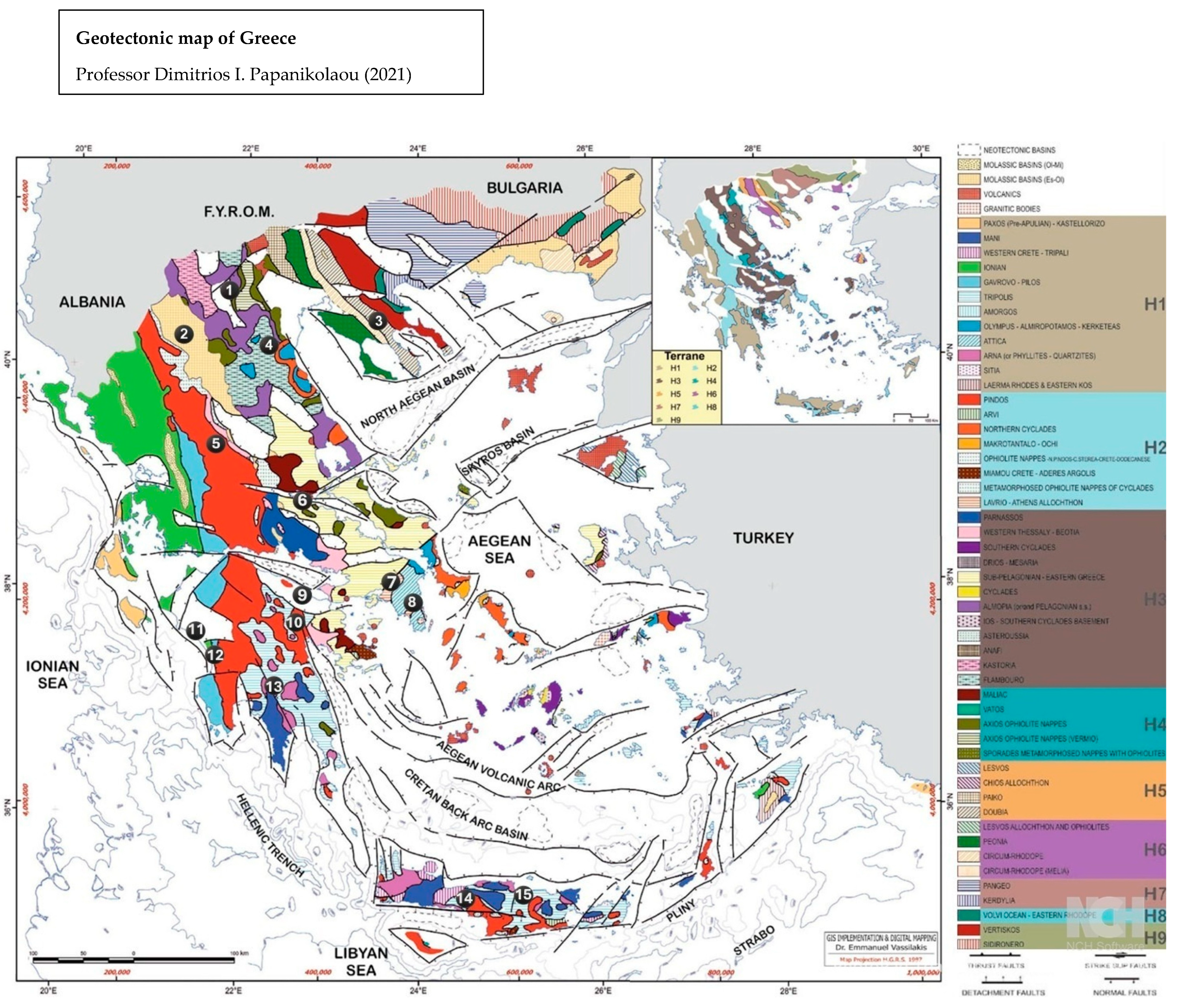
  66. Papanikolaou, D. The Geology of Greece; Regional Geology Reviews Series; Springer: Dordrecht, The Netherlands, 2021. [Google Scholar] [CrossRef]
  67. Economidis, S.P.; Banarescu, P. The distribution and origins of freshwater fishes in the Balkan Peninsula, Especially in Greece. Hydrobiology 1991, 76, 257–284. [Google Scholar] [CrossRef]
  68. Garcia-Guixé, E.; Subirà, M.E.; Marlasca, R.; Richards, M.P. δ13C and δ15N in ancient and recent fish bones from the Mediterranean Sea. J. Nord. Archaeol. Sci. 2010, 17, 83–92. [Google Scholar]
  69. Vika, E.; Theodoropoulou, T. Re-investigating fish consumption in Greek antiquity: Results from δ13C and δ15N analysis from fish bone collagen. J. Archaeol. Sci. 2012, 39, 1618–1627. [Google Scholar] [CrossRef]
  70. Papathanassiou, A.; Sherry, C.F.; Richards, P.M. Archaeodiet in the Greek World: Dietary Reconstruction from Stable Isotope Analysis; ASCSA Publications: Athens, Greece, 2015; 224p. [Google Scholar]
  71. Richards, M.; Karavanić, I.; Pettitt, P.; Miracle, P. Isotope and faunal evidence for high levels of freshwater fish consumption by Late Glacial humans at the Late Upper Palaeolithic site of Šandalja II, Istria, Croatia. J. Archaeol. Sci. 2015, 61, 204–212. [Google Scholar] [CrossRef]
  72. Panagiotopoulou, E. Reconstructing Diet, Tracing Mobility: Ιsotopic Approach to Social Change During the Transition from the Bronze to the Early Iron Age in Thessaly, Greece. Ph.D. Thesis, University of Groningen, Groningen, The Netherlands, 2018. [Google Scholar]
  73. Vika, E. Strangers in the grave? Investigating local provenance in a Greek Bronze Age mass burial using δ34S analysis. J. Archaeol. Sci. 2009, 36, 2024–2028. [Google Scholar] [CrossRef]
  74. Bocherens, H.; Drucker, D. Trophic level isotopic enrichment of carbon and nitrogen in bone collagen: Case studies from recent and ancient terrestrial ecosystems. Int. J. Osteoarchaeol. 2003, 13, 46–53. [Google Scholar] [CrossRef]
  75. Jim, S.; Ambrose, S.H.; Evershed, R.P. Stable carbon isotopic evidence for differences in the dietary origin of bone cholesterol, collagen and apatite: Implications for their use in palaeodietary reconstruction. Geochim. Cosmochim. Acta 2003, 68, 61–72. [Google Scholar] [CrossRef]
  76. Warinner, C.; Tuross, N. Alkaline cooking and stable isotope tissue-diet spacing in swine: Archaeological implications. J. Archaeol. Sci. 2009, 36, 1690–1697. [Google Scholar] [CrossRef]
  77. Fernandes, R.; Nadeau, M.-J.; Grootes, P.M. Macronutrient-based model for dietary carbon routing in bone collagen and bioapatite. Archaeol. Anthropol. Sci. 2012, 4, 291–301. [Google Scholar] [CrossRef]
  78. Froehle, A.W.; Kellner, C.M.; Schoeninger, M.J. FOCUS: Effect of diet and protein source on carbon stable isotope ratios in collagen: Follow up to Warinner and Tuross (2009). J. Archaeol. Sci. 2010, 37, 2662–2670. [Google Scholar] [CrossRef]
  79. Howland, M.R.; Corr, L.T.; Young, S.M.M.; Jones, V.; Jim, S.; Van Der Merwe, N.J.; Mitchell, A.D.; Evershed, R.P. Expression of the dietary isotope signal in the compound-specific δ13C values of pig bone lipids and amino acids. Int. J. Osteoarchaeol. 2003, 13, 54–65. [Google Scholar] [CrossRef]
  80. Richards, M.P.; Fuller, B.T.; Hedges, R.E.M. Sulphur isotopic variation in ancient bone collagen from Europe: Implications for human palaeodiet, residence mobility, and modern pollutant studies. Earth Planet. Sci. Lett. 2001, 1919, 185–190. [Google Scholar] [CrossRef]
  81. Richards, M.; Smith, C.; Nehlich, O.; Grimes, V.; Weston, D.; Mittnik, A.; Krause, J.; Dobney, K.; Tzedakis, Y.; Martlew, H. Finding Mycenaeans in Minoan Crete? Isotope and DNA analysis of human mobility in Bronze Age Crete. PLoS ONE 2022, 17, e0272144. [Google Scholar] [CrossRef]
  82. Dotsika, E.; Poutoukis, D.; Raco, B.; Psomiadis, D. Stable isotope composition of Hellenic bottled waters. J. Geochem. Explor. 2010, 107, 299–304. [Google Scholar] [CrossRef]
  83. Gamaletsos, P.; Godelitsas, A.; Dotsika, E.; Tzamos, E.; Göttlicher, J.; Filippidis, A. Geological sources of As in the environment of Greece: A review. In Threats to the Quality of Groundwater Resources: Prevention and Control. The Handbook of Environmental Chemistry; Scozzari, A., Dotsika, E., Eds.; Springer: Berlin/Heidelberg, Germany, 2013; pp. 77–113. [Google Scholar] [CrossRef]
  84. Siron, C.R.; Rhys, D.; Thompson, J.F.; Baker, T.; Veligrakis, T.; Camacho, A.; Dalampiras, L. Structural Controls on Porphyry Au-Cu and Au-Rich Polymetallic Carbonate-Hosted Replacement Deposits of the Kassandra Mining District, Northern Greece. Econ. Geol. 2018, 113, 309–345. [Google Scholar] [CrossRef]
  85. Höss, A.; Haase, K.M.; Keith, M.; Klemd, R.; Melfos, V.; Gerlach, L.; Pelloth, F.; Falkenberg, J.J.; Voudouris, P.; Strauss, H.; et al. Magmatic and hydrothermal evolution of the Skouries Au-Cu porphyry deposit, northern Greece. Ore Geol. Rev. 2024, 173, 106233. [Google Scholar] [CrossRef]
  86. Peterson, B.J.; Howarth, R.W.; Garritt, R.H. Multiple Stable Isotopes Used to Trace the Flow of Organic Matter in Estuarine Food Webs. Science 1985, 227, 1361–1363. [Google Scholar] [CrossRef]
  87. Anagnostopoulou, F. Investigation of Climatic Variable’s Spatial Distribution in Greece. Postgraduate Thesis, NTUA, Athens, Greece, 2006. Available online: https://www.itia.ntua.gr/en/docinfo/872 (accessed on 15 May 2024).
  88. Weber, Y.; De Jonge, C.; Rijpstra, W.I.C.; Hopmans, E.C.; Stadnitskaia, A.; Schubert, C.J.; Lehmann, M.F.; Damsté, J.S.S.; Niemann, H. Identification and carbon isotope composition of a novel branched GDGT isomer in lake sediments: Evidence for lacustrine branched GDGT production. Geochim. Cosmochim. Acta 2015, 154, 118–129. [Google Scholar] [CrossRef]
  89. Frydas, D.; Keupp, H.; Bellas, S. Stratigraphical investigations based on calcareous and siliceous phytoplankton assemblages from the Upper Cenozoic deposits of Messara Basin, Crete, Greece. Z. Dtsch. Ges. Geowiss. 2008, 159, 415–438. [Google Scholar] [CrossRef]
  90. Graven, H.; Allison, C.E.; Etheridge, D.M.; Hammer, S.; Keeling, R.F.; Levin, I.; Meijer, H.A.J.; Rubino, M.; Tans, P.P.; Trudinger, C.M.; et al. Compiled records of carbon isotopes in atmospheric CO2 for historical simulations in CMIP6. Geosci. Model Dev. 2017, 10, 4405–4417. [Google Scholar] [CrossRef]
  91. Bellas, S.M.; Keupp, H. Contribution to the late neogene stratigraphy of the ancient gortys area (southern central Crete, Greece). Bull. Geol. Soc. Greece 2017, 43, 579. [Google Scholar] [CrossRef]
  92. Bird, Μ.Ι.; Crabtree, A.S.; Haig, J.; Ulm, S.; Wurster, C.M. A global carbon and nitrogen isotope perspective on modern and ancient human diet. Anthropology 2021, 118, e2024642118. [Google Scholar] [CrossRef] [PubMed]
Figure 2. Carbon values (δ13C) versus temperature. The inserted figure illustrates a temperature map of Greece.
Applsci 15 04351 g002
Figure 3. δ15N versus δ13C in different plants from Greece.
Applsci 15 04351 g003
Figure 4. The δ15N versus δ13C of various aromatic species and wild olives.
Applsci 15 04351 g004
Figure 5. δ15N of Greek plants versus precipitation (mean values) [48].
Applsci 15 04351 g005
Figure 6. Median of δ34S vs. δ15Ν isotopic data for plants from various localities of Greece.
Applsci 15 04351 g006
Figure 7. Geological map of Greece illustrating the sampling areas within particular massifs, units, and belts, as described briefly below (names of sampling locations are captioned in Figure 1; modified after Papanikolaou (2021) [66]). The geotectonic units and the tectonostratigraphic terranes are shown in the corresponding legend at the rightmost part of the map. According to Papanikolaou (2021) and references therein [66], the Rhodope Massif mainly consists of metamorphic and igneous rocks, such as gneisses, marbles, chlorite mica and mica schists, amphibolites, migmatites, granites, granodiorites, rhyolites, andesites, and dacites. Apart from metamorphic rocks (mica schists and amphibolitic schists and amphibolites), the Serbo-Macedonian Massif comprises massive outcrops of ophiolites and granites, granodiorites and diorites. The Circum-Rhodope Unit includes sandstones, quartzites, and schists, as well as volcano-sedimentary formations, such as limestones, marbles, crystalline limestones, flysch, cherts, schists, phyllites, and gneisses. The Axios/Vardar Belt is mainly observed in the form of ophiolite complexes, while volcanic schists, phyllites, marbles, cherts, sandstones, and limestones can be observed. The Peonia, Paikon, and Almopia Units can be distinguished. The Axios Belt also has clear volcanic activity features. The Pelagonian Unit is composed of gneisses, gneisses–schists, amphibolites, and granite intrusions. Marbles, phyllites, schists, and sandstones as well as limestones and dolomites are also present. Massive ophiolite tectonic nappes can be observed. The Attic–Cycladic Massif consists of marbles, dolomites, and mica and amphibolitic schists. The metamorphic evolution of the Attic–Cycladic Massif is mainly characterized by massive granitic intrusions. The Parnassos Unit is characterized by the presence of massive carbonates (limestones and dolomites). These shallow-water carbonate platforms host the three bauxitic stratigraphic horizons, B1, B2, and B3. The Pindos Unit is mainly composed of limestones, dolomites, volcano-sedimentary formations, radiolarites marls, pelites, sandstones, and cherts. The massive ophiolitic sequence in Greece is thrust onto the Pindos unit by obduction. Limestones and dolomites are the main formations in the Gavrovo–Tripolis Unit. An HP metamorphic unit—also known as a “Phyllite-Quartzite (PQ) nappe”—is occurring beneath the Gavrovo–Tripolis carbonate series. The Ionian Unit is mainly characterized by the presence of a carbonate stratigraphic sequence (neritic and pelagic limestones, dolomites, slates, and cherts) overlying the evaporites. This unit is thrust onto the Paxos (or Pre-Apulian) Unit, and it is also associated with a metamorphic “Plattenkalk” (platy-like limestones) series (also known as “Mani Unit” or Talea Ori). The Paxos Unit is a typical shallow-water carbonate autochthonous platform overlying evaporites (e.g., gypsum). It can only be observed in the Paxos, Lefkada, Kefalonia, and Zakynthos Islands.
Applsci 15 04351 g007
Figure 8. δ15N versus δ13C of the studied plants and mammals from different localities in Greece.
Applsci 15 04351 g008
Figure 9. Median of δ15Ν vs. δ34S isotopic data for (1) cattle from Chalkidiki; (2) cattle from Crete; (3) sheep from Chalkidiki; (4) sheep from Crete; (5) cows from Sparta; and (6) sheep from Sparta.
Applsci 15 04351 g009
Figure 10. Median of δ34S vs. δ15Ν data for mammals from different areas of Greece.
Applsci 15 04351 g010
Figure 11. The boxes, δ34S versus δ15N, indicate terrestrial (brown—mammals; green–plants), freshwater (light blue), and marine (deep blue) reservoirs. The black box represents C4 plants [72,73,80,81].
Applsci 15 04351 g011
Figure 12. The boxes, δ34S versus δ13C values, indicate terrestrial (brown—mammals; green—plants), freshwater (light blue), and marine (deep blue) reservoirs. The black boxes are C4 plants. All modern carbon isotopic values have been calibrated to ancient ones [72,73,80,81].
Applsci 15 04351 g012
Table 4. Stable isotopes of the δ13C, δ15N, and δ34S of fish and faunal, old and recent from Greece.
Fish/Faunal Ageδ13C.
‰. V-PDB
δ15N.
‰. V-Air
δ34S.
‰. V-CD
Authors
Pandora, Pagellus erythrinus (bones)Recent−13.1 to −14.110.3 to 10.1 [68]
Moray eel, Muraena Helena (bones)Recent−13.710.8
Barracuda, Sphyraena sphyraena (bones) Recent−13.7 to −147.9 to 7.8
Dusky grouper, Epinephelus marginatus (bones)Recent−8.4 to −8.311.4 to 10.7
Marine fish (bones)Ancient−10.1 to −19.211.6 to 6.1 [69]
Freshwater fish (bones)Ancient−11.9 to −20.810.9 to 4.9
Marine fish (bones)Ancient−11 to −1419 to 7 [71]
Marine fish (bass, bones)Ancient−11.4 to −10.311 to 8.44 [69]
Faunal (bones)Ancient−18.3 to −20.57 to 4.29.9 το 14.7[73]
Faunal (bones)Ancient−18.5 to −20.18.2 to 2.28.2 to 2.1[71]
Faunal (bones)Ancient−19.9 to −20.43.9 to 5.715 to 18.2[52]
Table 5. δ 34S of recent and archaeological mammals.
SpeciesAgeδ34S,
‰. V-CD
sdAuthors
All herbivores mammal samplesRecent7.501.47This work
All herbivores mammal samplesOld, from Greece12.454.53[72,73]
All herbivores mammal samplesClassical site, Thebes13.302.18[73]
All herbivores mammal samplesEarly Iron Age, Thessaly7.902.50[80]
All herbivores mammal samplesMinoan, Chamalevri17.71.72[80]
Cattle, from Crete
(one sample)
Minoan, Chamalevri18.20 [80]
All herbivores mammal samples Earl Minoan to Roman, Crete11.602,45[81]
Sheep, Ovi sariesMiddle to Late Minoan, Chamalevri12.602.72
Sheep, Ovi sariesMiddle Minoan, Apodoulou 10.400.63
Cattle, from CreteRecent9.602.16This work
Disclaimer/Publisher’s Note: The statements, opinions and data contained in all publications are solely those of the individual author(s) and contributor(s) and not of MDPI and/or the editor(s). MDPI and/or the editor(s) disclaim responsibility for any injury to people or property resulting from any ideas, methods, instructions or products referred to in the content.

