Regional Seismicity of the Northeastern Tibetan Plateau Revealed by Crustal Magnetic Anomalies

Abstract

The northeastern Tibetan Plateau (NETP) is located at the front of the northeastward expansion of the Tibetan Plateau and is a tectonically active region with complex faults and intense seismicity. In this study, based on the high-order geomagnetic field model EMM2017, the crustal magnetic anomalies and Curie point depths (CPDs) in the NETP and adjacent areas were investigated. The relationship between the magnetic anomalies, CPDs, and seismic activity was assessed. The results show that strong earthquakes occur mainly in areas where the magnetic anomalies are negative or have a strong-to-weak transition. The CPD is located at 18–42 km. In the NETP, a shallow CPD corresponds to high heat flow. In contrast, in surrounding areas, a deep CPD corresponds to low heat flow. The northeast area from Bayan Har to the Qilian orogenic belt, and the region with a deep CPD in the Qaidam Basin, record the northeastward flow of the Tibetan Plateau. High-magnitude earthquakes are associated with depth changes in the CPD and areas with a shallow CPD. The frequent seismic activity in the NETP can be attributed to the northeastward flow of the Tibetan Plateau caused by a deep heat flux. The results can be used as a reference for the prediction of strong regional earthquakes.

1. Introduction

Earthquakes are the most dangerous of all natural disasters. Strong earthquakes can result in severe and extensive structural and non-structural damage to the built environment [1,2]. Due to the considerable loss of life and damage caused by strong earthquakes, a variety of studies have been conducted, such as in building earthquake warning systems, as well as in the strengthening of structures and disaster management systems. With the advent of remote sensing satellites (e.g., the DEMETER, Swarm, and CSES-01 satellites), the number of statistical studies related to earthquake precursors has increased significantly. However, there have still been no reliable scientific reports on successful earthquake prediction.

The northeastern Tibetan Plateau (NETP) is unique in its geographical location and tectonic activity. It is located in the northernmost part of the Tibetan Plateau at the junction of the Tibetan Plateau, Tarim Basin, Alxa–Ordos Block, and Sichuan Basin (Figure 1). The topography changes rapidly, and the crustal structure is complex due to the collision between the Indian and Eurasian plates being blocked by the Yangtze and Ordos blocks [3]. The NETP is undergoing intense northeast-directed crustal deformation, crustal shortening, and lithospheric thickening, and it is characterized by the highest level of seismicity in mainland China [4,5]. There have been nearly 60 earthquakes of Ms ≥ 6.0 in the region in historic times [6]. As such, the NETP is an ideal region for investigating the block interactions, as well as seismotectonics.

The crustal magnetic field (i.e., crustal magnetic anomalies) is generated by magnetic rocks between Earth’s surface and the Curie isothermal surface (also called the Curie surface) [7]. The field is affected by factors such as geological structures, rock magnetic properties, temperature, and stress [8]. Crustal magnetic anomalies record changes in these factors [9,10]. Crustal magnetic anomaly data have been used to estimate the Curie point depth (CPD) [11,12,13,14], which is the depth at which ferromagnetic minerals are transformed into a paramagnetic state due to the increasing temperature. The interface between these phases is termed the Curie surface. Magnetite is the dominant crustal magnetic mineral as a result of its magnetic susceptibility and abundance, and it has a Curie point of 580 °C. Therefore, the CPD is often interpreted to be the depth of the 580 °C isotherm. For this reason, the CPD provides robust constraints on the thermal structure of the crust [11]. Moreover, the thermal structure may contribute to the generation and occurrence of earthquakes [14]. Information regarding crustal magnetic anomalies and the CPD obtained from crustal magnetic anomaly data can provide important insights into seismic activity and regional tectonism.

Previous studies have used crustal magnetic anomalies to study earthquake activity. Wei et al. (2012) found that magnetic anomalies in China have a close relationship with seismic structures [15]. Yan et al. (2016) studied magnetic anomalies in the areas of the 2008 Wenchuan earthquake (Ms = 7.8; Sichuan) and Longmenshan Fault [16]. Wen et al. (2021) used the NGDC-720 geomagnetic field model to study the relationship between crustal magnetic anomalies and strong earthquake activity in the southern part of the China North–South Seismic Belt [17]. In addition, the CPD is closely related to seismicity [18,19,20,21]. However, different tectonic units exhibit different relationships between the CPD and seismicity [21]. The NETP is a tectonically active region with complex faults and intense seismicity. So far, works on revealing the regional seismicity of the NETP according to the crustal magnetic anomalies are still lacking.

Satellite, ground, oceanic, and aeromagnetic surveys have been used to observe the geomagnetic field [7]. In particular, magnetic surveys by satellites (e.g., Ørsted, CHAMP, SAC-C, SWARM, CSES-01, and MACAU-01) have accumulated a large amount of geomagnetic field data [22], leading to a series of high-quality geomagnetic field models being developed [23,24,25]. In 2017, the geomagnetic field model EMM2017 was established by combining data from satellite, ground, oceanic, and aeromagnetic surveys (https://www.ncei.noaa.gov/products/enhanced-magnetic-model (accessed on 1 January 2025)). In that model, the order of the spherical harmonic functions is up to 790, and the resolvable spatial wavelength is as fine as 51 km. This model provides valuable data for the analysis of regional crustal magnetic anomalies.

The NETP is a region where different tectonic blocks collide and intersect, and large earthquakes occur frequently. However, the mechanisms that generate the earthquakes remain unclear. In this study, we investigated the relationship between crustal magnetic anomalies and seismic activity in the NETP and adjacent areas using the EMM2017 model. We inverted the CPD through a spectral analysis of the magnetic anomalies and compared it with the regional heat flow, crustal structure, and seismicity.

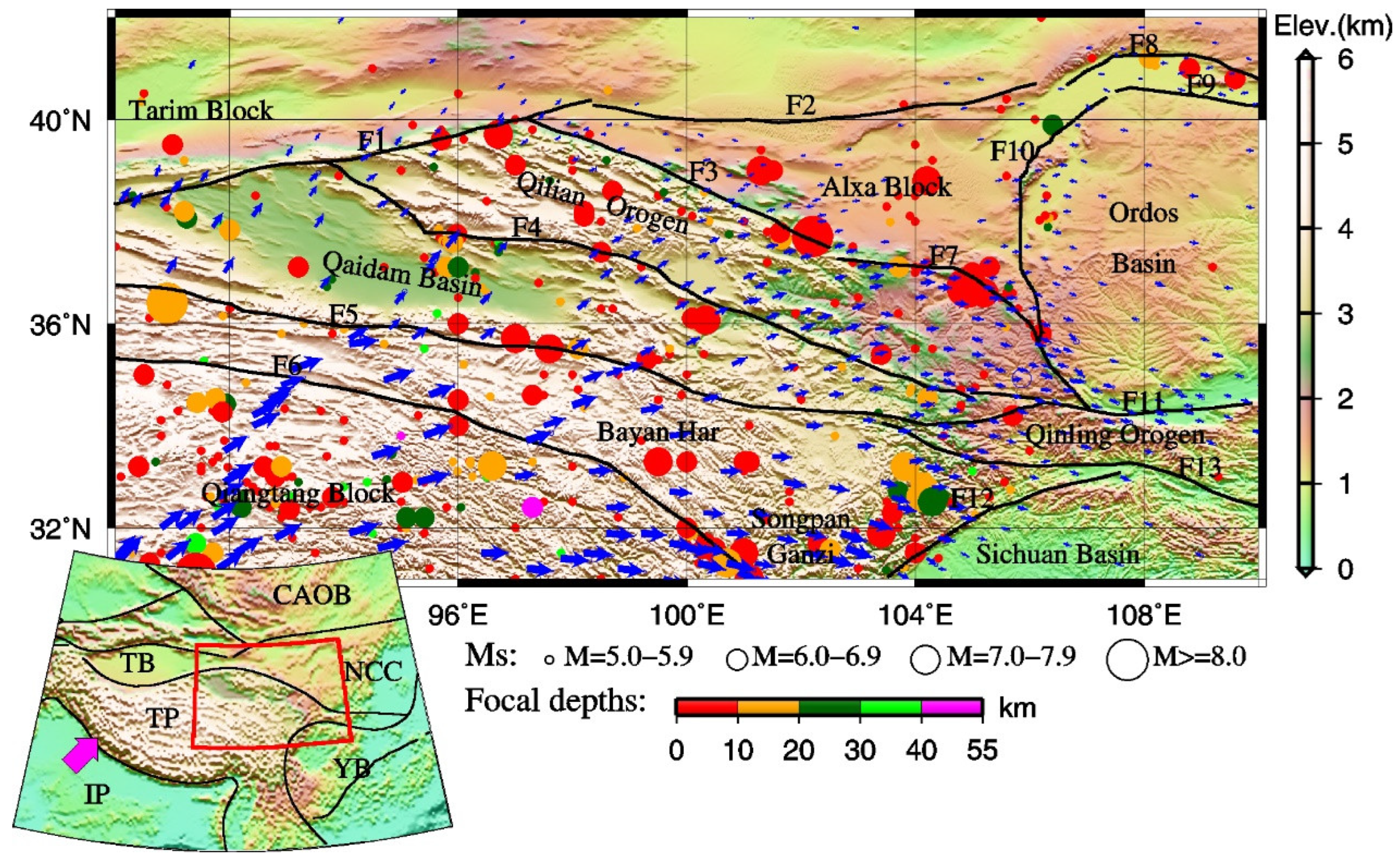
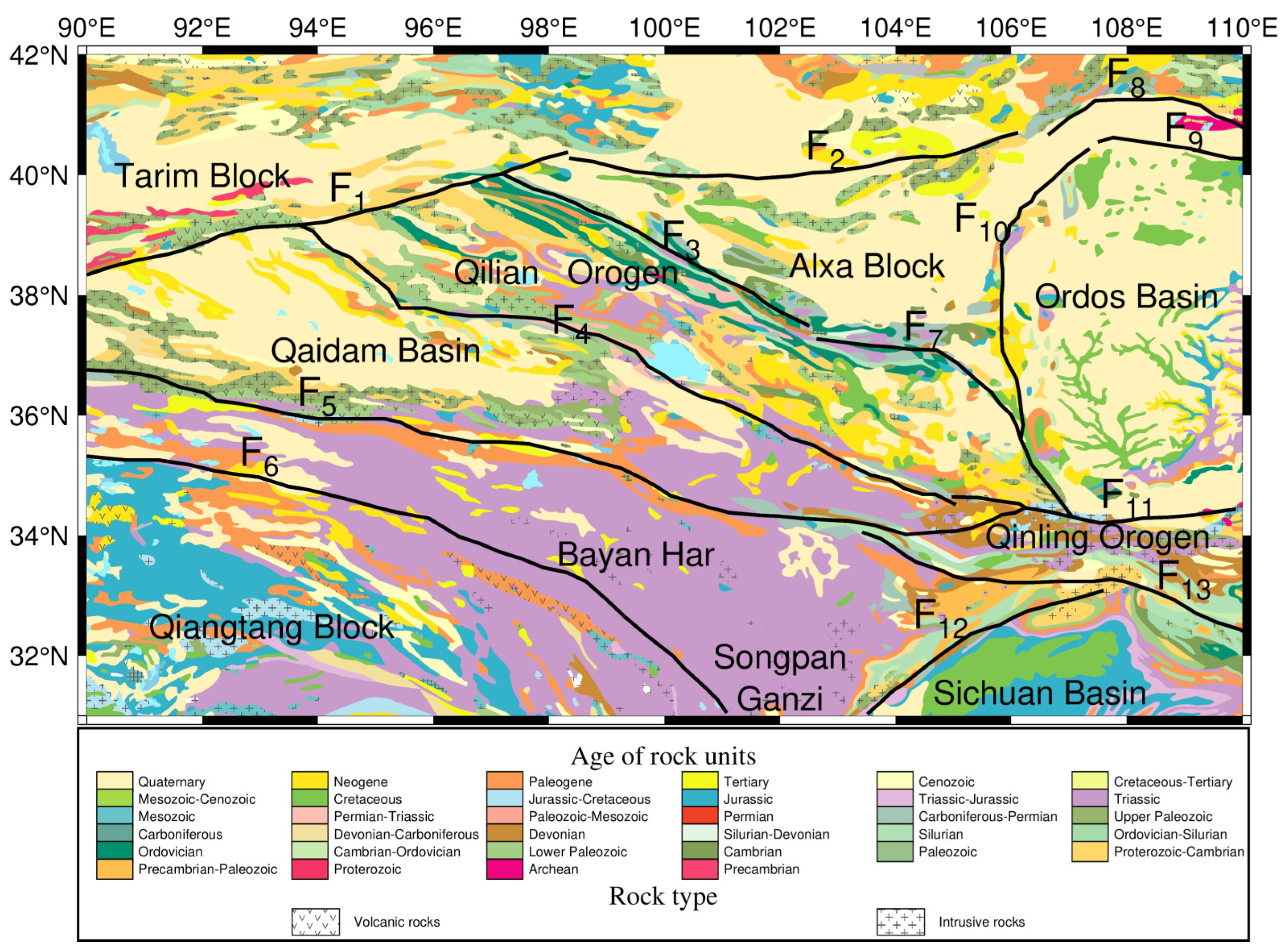
2. Geological Setting

The NETP is bounded by the Jinsha River suture to the south, the Altyn Tagh Fault to the north, and the North Qilian–Haiyuan Fault to the northeast. It is an area of collisions between blocks, intracontinental convergence, and strong crustal deformation. The northern part of the NETP comprises the relatively stable Tarim and Alax blocks, the eastern NETP is the Ordos Basin, the southeastern NETP is the South China Block, and the southern NETP is the Qiangtang Block. Several secondary blocks (i.e., the Qilian, Qaidam, Bayan Har, and Qinling blocks) converge on the NETP, resulting in remote effects (complex and strong–moderate deformation) as a result of continent–continent collisions that have occurred during the Cenozoic. Northeastward compression has resulted in the formation of a series of strike-slip faults, such as the Altyn Tagh, Haiyuan, Kunlun, and Longmengshan faults. The tectonics of this area are closely related to the India–Asia collision that began at ca. 70–50 Ma [26]. Continent–continent collision has resulted in significant crustal thickening.

The NETP and the adjacent regions consist of several tectonic units, including the widely spread Precambrian units, Caledonian units, Variscan units, Indosinian units, and Yanshanian units, as well as basins and igneous units [4]. As shown in Figure 2, the tectonic units, sedimentary basins, and igneous units are divided by suture zones and fault belts. As the northern boundary of the Tibetan plateau, the Qilian orogen, which was developed at the southern margin of the North China craton before it was offset by the Altyn Tagh fault in the Cenozoic, consists of complexly deformed early Palaeozoic arcs [26], and it is undergoing ∼NNE–SSW horizontal shortening at a rate of about 12 mm yr⁻¹ [27]. The Qaidam basin in the south comprises a broad early Palaeozoic arc and a younger and narrower late Permian-to-Triassic arc [26]. The Songpan-Ganzi block, to the south of the eastern Kunlun fault, was an accretionary prism formed during the northward subduction of the oceanic Qiangtang lithosphere beneath the Tarim-North China block [4].

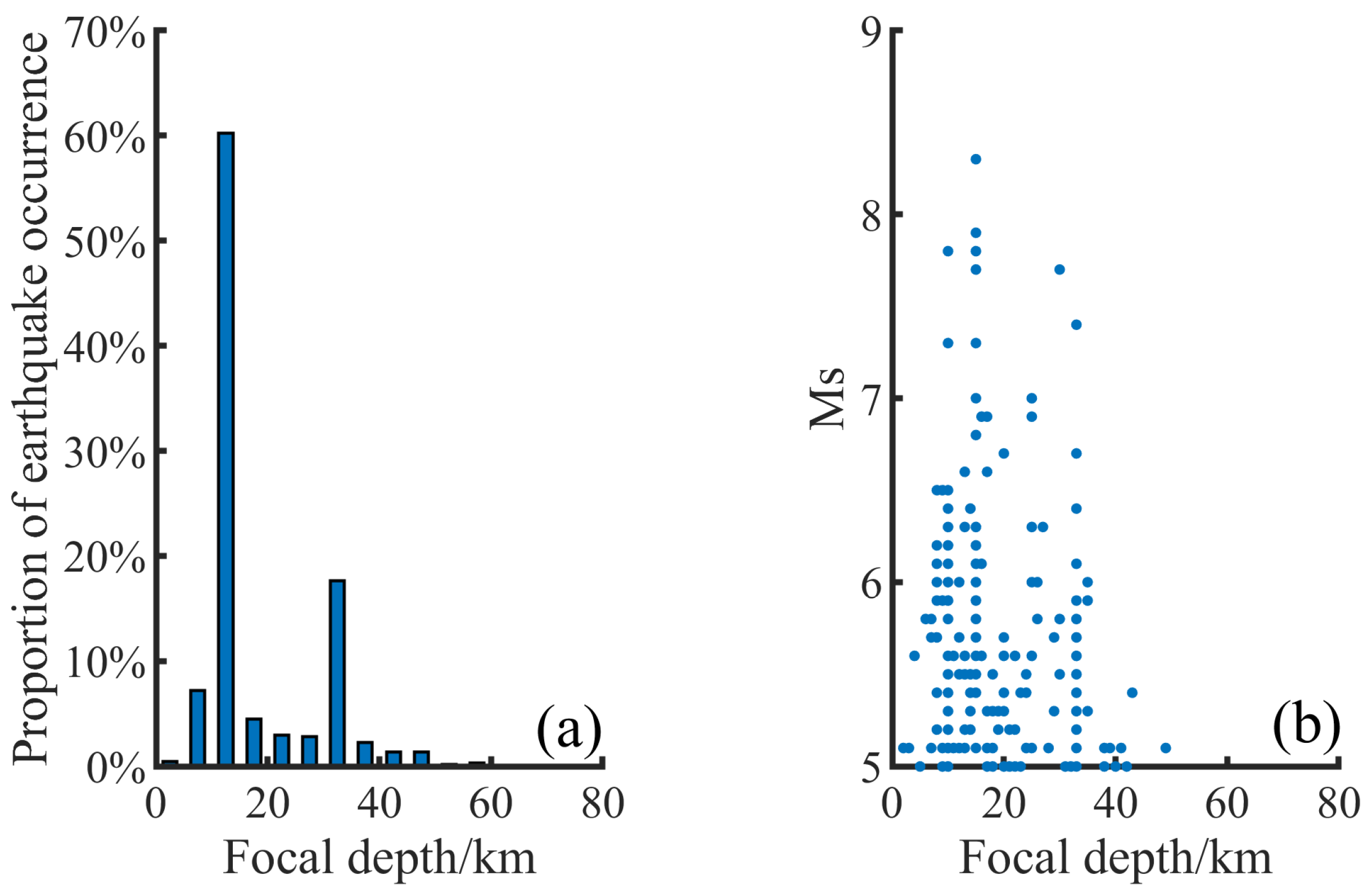
3. Regional Seismicity

The NETP is characterized by the highest level of seismicity in mainland China. The northern part of the China North–South Seismic Belt is located in this region, and large active faults and frequent seismic activity are indicative of strong tectonic deformation. We compiled seismic data for earthquakes of Ms ≥ 5 since 1900 from the China Earthquake Networks Center, National Earthquake Data Center, and United States Geological Survey (

Table 1. The earthquakes occurring in the study areas of Ms ≥ 5.0 since 1900.

NO.	Date	Lon./(°)	Lat./(°)	Ms	Depth/(km)	NO.	Date	Lon./(°)	Lat./(°)	Ms	Depth/(km)
1	16 December 1920	36.89	105.61	8.5	15	191	12 September 2000	35.33	99.3	5.1	10
2	25 December 1920	37.24	105.48	6.8	15	192	12 September 2000	35.39	99.34	6.1	10
3	24 March 1923	31.3	100.75	7	15	193	13 September 2000	34.14	95.12	5	33
4	22 May 1927	37.65	102.49	8.0	15	194	20 September 2000	35.42	99.55	5.1	33
5	7 March 1928	37.67	102.13	6.2	15	195	28 October 2000	32.67	92.23	5.1	33
6	13 July 1930	37.97	98.26	6.5	10	196	30 October 2000	32.74	92.24	5.2	33
7	25 December 1932	39.5	96.62	7.9	15	197	26 November 2000	35.87	90.55	5.4	33
8	25 August 1933	32.01	103.68	7.3	15	198	10 July 2001	39.02	97.99	5	33
9	20 January 1934	41.14	108.62	6.3	15	199	25 July 2001	33.17	95.6	5.5	33
10	26 July 1935	33.17	100.94	6.2	15	200	14 November 2001	35.65	93.96	5	10
11	7 February 1936	35.44	103.19	6.8	15	201	14 November 2001	35.75	94.02	5.1	10
12	7 January 1937	35.43	97.76	7.8	15	202	14 November 2001	35.61	93.98	5.2	10
13	17 March 1947	33.48	99.53	7.3	15	203	14 November 2001	35.6	94.49	5.3	10
14	18 June 1950	34.95	99.77	5.8	30	204	14 November 2001	35.65	93.88	5.4	10
15	21 August 1950	33.04	91.48	6	15	205	14 November 2001	35.73	93.38	5.6	10
16	17 September 1950	32.44	93.96	5.6	15	206	14 November 2001	35.95	90.54	8.1	10
17	30 October 1950	33.17	95.85	5.7	15	207	18 November 2001	35.71	93.69	5.4	10
18	1 August 1951	31.54	95.31	5.5	15	208	18 November 2001	35.73	93.69	5.6	10
19	18 November 1951	31.06	91.26	7.7	30	209	19 November 2001	35.76	93.67	5.4	10
20	26 December 1951	39.49	95.53	6.2	15	210	30 November 2001	36.07	91.12	5.2	10
21	26 December 1951	31.24	90.78	6.3	15	211	1 December 2001	35.58	93.93	5.1	10
22	23 January 1952	39.73	95.44	6	35	212	8 December 2001	35.73	92.77	5.3	10
23	3 February 1952	33.98	93.8	5.5	15	213	7 February 2002	37.93	92.15	5	18
24	6 February 1952	39.59	98.66	5.8	15	214	22 May 2002	36.99	95.34	5	10
25	15 June 1952	31.37	90.92	5.9	15	215	29 June 2002	34.13	94.5	5.6	33
26	14 September 1952	34.35	91.86	6	15	216	27 September 2002	33.36	93.57	5.1	33
27	1 October 1952	36.52	92.1	5.7	15	217	19 October 2002	35.65	93.13	5.1	33
28	5 October 1952	37.01	93.2	6.1	15	218	26 October 2002	35.14	96.1	5.4	33
29	31 October 1952	33.22	101.16	6.2	15	219	14 December 2002	39.74	97.44	5.6	22
30	23 April 1953	31.05	96.87	6	10	220	11 February 2003	32.51	93.79	5.1	33
31	11 February 1954	38.96	101.22	7	25	221	17 April 20038	37.53	96.48	6.4	14
32	31 July 1954	38.62	104.15	6.9	25	222	3 May 2003	37.48	96.54	5.1	10
33	7 February 1958	31.46	104.01	6	25	223	20 May 2003	32.68	93.09	5.2	33
34	30 April 1958	38.37	103.97	5.5	30	224	24 May 2003	32.61	92.34	5.1	49
35	27 April 1959	33.22	92.72	5.9	15	225	24 May 2003	32.59	92.43	5.1	33
36	21 August 1959	39.22	104.28	5.4	15	226	3 July 2003	35.71	93.71	5	10
37	28 September 1960	32.44	95.86	5.6	15	227	18 July 2003	38.91	98.57	5	10
38	9 November 1960	32.71	103.63	6.3	25	228	6 October 2003	38.86	100.01	5	10
39	4 December 1961	33.34	95.25	6.1	16	229	10 October 2003	39.58	98.22	5.1	10
40	21 May 1962	36.93	95.93	6.6	17	230	25 October 2003	38.35	101.04	5.2	10
41	17 December 1962	37.95	106.19	5.7	20	231	25 October 2003	38.4	100.95	5.8	10
42	19 April 1963	35.61	96.99	6.7	20	232	25 October 2003	38.38	100.98	5.8	10
43	15 August 1967	31.08	93.64	5.7	20	233	13 November 2003	34.71	103.83	5.1	10
44	30 August 1967	31.59	100.26	5.8	10	234	12 December 2003	37.63	94.59	5.1	10
45	30 August 1967	31.63	100.26	6.4	10	235	24 February 2004	37.49	96.83	5.1	41
46	22 December 1968	36.31	101.77	5.6	25	236	6 March 2004	33.29	91.95	5	38
47	24 March 1971	35.45	98.14	6	10	237	7 March 2004	31.64	91.24	5.6	11
48	3 April 1971	32.16	95.04	5.8	15	238	16 March 2004	37.56	96.67	5.2	14
49	22 May 1971	32.3	92.1	5.6	10	239	4 May 2004	37.47	96.91	5.2	10
50	22 July 1972	31.36	91.44	5.9	10	240	4 May 2004	37.51	96.76	5.5	14
51	30 August 1972	36.62	96.56	5.5	18	241	10 May 2004	37.49	96.6	5.6	10
52	15 January 1973	40.43	91.07	5.1	13	242	24 August 2004	32.54	92.19	5.5	10
53	6 February 1973	31.7	100.02	5.1	33	243	7 September 2004	34.68	103.78	5.2	10
54	6 February 1973	31.4	100.58	7.4	33	244	10 December 2004	35.68	93.18	5	10
55	7 February 1973	31.46	100.29	5.8	33	245	3 March 2009	31.8	104.79	5.1	10
56	23 March 1973	31.88	100.06	5.4	33	246	12 March 2009	32.39	105.1	5.3	10
57	9 June 1973	39.42	95.41	5	33	247	29 June 2009	31.43	104.01	5.3	10
58	16 June 1973	37.71	95.64	5.4	33	248	16 July 2009	38.87	101.31	5.1	15
59	21 July 1973	35.55	96.06	5.2	33	249	28 August 2009	37.69	95.78	5	10
60	11 August 1973	33	104.02	6.1	33	250	28 August 2009	37.65	95.71	5.6	4
61	9 September 1973	31.48	100	5.2	33	251	28 August 2009	37.68	95.77	5.6	16
62	9 September 1973	31.65	100.01	5.5	33	252	28 August 2009	37.7	95.72	6.3	13
63	9 October 1973	31.69	99.76	5	33	253	29 August 2009	37.64	95.72	5.2	10
64	15 January 1974	32.91	104.2	5.7	33	254	30 August 2009	37.67	95.65	5.4	10
65	22 September 1974	33.58	102.45	5.1	33	255	31 August 2009	37.64	95.89	5.3	10
66	16 November 1974	33.05	103.98	5.2	33	256	28 August 2009	37.61	95.83	5.8	6
67	4 January 1975	38.53	97.51	5.4	33	257	1 September 2009	37.68	95.88	5	10
68	14 March 1975	34.01	95.48	5.1	33	258	17 September 2009	37.64	95.94	5.1	10
69	5 May 1975	33.09	92.92	6.1	33	259	18 September 2009	37.65	95.59	5	5
70	7 November 1975	33.29	95.33	5.2	33	260	18 September 2009	37.65	95.6	5.1	7
71	16 August 1976	32.93	104.26	5	33	261	2 October 2009	39.49	96.07	5	10
72	16 August 1976	32.75	104.16	6.9	16	262	19 October 2009	31.97	104.61	5.1	38
73	19 August 1976	32.89	104.19	5.4	33	263	23 October 2009	34.9	99.46	5.1	39
74	21 August 1976	32.57	104.25	6.4	33	264	29 October 2009	32.52	105.24	5.2	14
75	23 August 1976	32.49	104.18	6.7	33	265	4 November 2009	37.65	95.76	5.1	3
76	1 September 1976	32.46	104.15	5.1	18	266	13 December 2009	41.72	94.32	5.4	10
77	20 September 1976	32.77	104.12	5	42	267	21 December 2009	37.53	96.64	5	10
78	22 September 1976	40.03	106.33	5.7	29	268	1 March 2010	32.3	105.17	5	38
79	17 December 1967	33.34	93.91	5.1	33	269	24 March 2010	32.52	92.83	5.4	20
80	1 January 1977	38.15	91.01	6.3	27	270	24 March 2010	32.51	92.71	5.7	7
81	19 January 1977	37.02	95.7	5.9	33	271	13 April 2010	33.17	96.55	6.9	17
82	19 October 1977	39.16	91.04	5.1	33	272	14 April 2010	33.07	96.62	5	10
83	7 December 1977	35.6	94.52	5	33	273	14 April 2010	33.13	96.55	5.2	10
84	12 July 1978	31.91	103.04	5.3	33	274	14 April 2010	32.93	96.86	5.4	23
85	16 August 1978	38.38	101.36	5	33	275	14 April 2010	33.2	96.45	6.1	8
86	17 November 1978	37.29	97.09	5	33	276	17 April 2010	32.51	92.83	5.3	35
87	2 February 1979	39.72	90.75	5	33	277	25 May 2010	31.15	103.55	5	10
88	29 March 1979	32.15	96.96	5.8	33	278	29 May 2010	33.17	96.07	5.8	7
89	24 August 1979	41.15	108.13	5.9	33	279	3 June 2010	33.3	96.09	5.1	10
90	28 September 1979	38.21	90.46	5	22	280	3 June 2010	33.34	96.15	5.5	24
91	2 December 1979	38.49	90.15	5.2	33	281	7 September 2010	33.28	96.31	5.1	2
92	6 March 1980	35.99	91.84	5	33	282	10 April 2011	31.37	100.76	5.4	43
93	1 June 1980	38.9	95.64	5.2	33	283	15 May 2011	32.5	105.42	5	10
94	12 July 1980	36.83	93.78	5.4	24	284	26 June 2011	32.45	95.95	5.3	29
95	9 June 1981	34.5	91.44	6	10	285	11 August 2011	37.66	95.69	5	10
96	7 November 1981	31.33	103.97	5.1	33	286	31 October 2011	32.53	105.32	5	40
97	15 June 1982	31.91	99.93	5.6	10	287	1 November 2011	34.54	104.17	5	32
98	27 March 1983	34.24	92.6	5	33	288	3 May 2012	40.51	98.53	5.2	10
99	15 June 1983	34.23	92.94	5.2	33	289	11 May 2012	37.74	102.05	5	10
100	25 December 1983	37.94	91.12	5	31	290	26 November 2012	40.41	90.36	5	10
101	5 January 1984	37.97	102.19	5.5	12	291	18 January 2013	31.06	99.55	5.4	8
102	17 February 1984	37.69	100.8	5.3	10	292	30 January 2013	32.92	94.68	5.2	22
103	14 June 1984	36.92	96.48	5	33	293	11 February 2013	38.48	92.37	5.3	17
104	28 July 1984	34.19	92.97	5.3	33	294	5 June 2013	37.6	95.93	5.1	9
105	23 November 1984	37.99	106.36	5.2	33	295	21 July 2013	34.51	104.26	5.9	8
106	16 January 1985	32.88	95.36	5	33	296	22 July 2013	34.53	104.18	5.4	10
107	24 June 1985	33.91	104.38	5	33	297	19 September 2013	37.75	101.51	5	21
108	11 August 1985	36.13	95.63	5.2	33	298	4 October 2013	32.01	104.48	5	10
109	20 August 1985	41.66	90.35	5.4	33	299	27 April 2014	38.41	93.04	5.1	17
110	20 August 1986	34.57	91.63	6.4	33	300	9 June 2014	32.5	105.18	5	17
111	26 August 1986	37.69	101.72	8.1	23	301	2 October 2014	36.37	97.77	5.1	12
112	26 August 1986	37.68	101.59	5.4	10	302	15 April 2015	39.75	106.4	5.4	10
113	26 August 1986	37.72	101.5	6	8	303	12 October 2015	34.3	98.23	5.1	11
114	16 August 1986	37.75	101.64	5.3	18	304	22 November 2015	37.99	100.35	5.1	13
115	16 September 1986	37.76	101.73	5.3	19	305	13 January 2016	32.65	91.63	5.2	10
116	9 November 1986	33.99	96.32	5	10	306	20 January 2016	37.64	101.59	5	10
117	20 November 1986	32.58	93.01	5	33	307	20 January 2016	37.67	101.64	5.9	9
118	20 November 1986	32.65	93.12	5.1	33	308	23 February 2016	32.06	95.04	5.1	10
119	22 November 1986	32.19	94.59	5	33	309	11 May 2016	32.02	95.03	5.2	8
120	20 December 1986	36.75	93.66	5.3	33	310	13 August 2016	37.71	101.55	5.2	21
121	7 January 1987	34.26	103.41	5.4	33	311	17 October 2016	32.9	94.88	5.9	35
122	25 February 1987	38.14	91.22	5	33	312	17 November 2016	32.69	96.15	5	10
123	25 February 1987	38.1	91.18	5.8	26	313	4 December 2016	32.42	92.12	5.2	10
124	10 August 1987	38.12	106.36	5.3	10	314	14 December 2016	38.58	90.05	5.1	10
125	3 January 1988	38.11	106.34	5.2	14	315	8 August 2017	33.19	103.86	6.5	9
126	10 January 1988	38.17	106.36	5.1	10	316	30 September 2017	32.28	105.04	5.1	10
127	5 November 1988	34.35	91.88	6.2	8	317	12 October 2017	32.07	95.05	5.1	10
128	25 November 1988	34.33	91.93	5.6	25	318	31 October 2017	34.91	103.29	5	10
129	26 December 1988	39.01	99.94	5.1	10	319	14 December 2017	35.15	101.88	5	9
130	1 March 1989	31.49	102.46	5	33	320	6 April 2018	34.56	96.52	5	18
131	13 May 1989	35.22	91.58	5.3	33	321	17 June 2018	38.86	94.92	5	10
132	22 September 1989	31.58	102.43	6.1	15	322	3 August 2018	34.94	92.16	5.2	19
133	2 November 1989	36.04	106.23	5	10	323	12 September 2018	32.72	105.66	5	10
134	14 January 1990	37.82	91.97	6	12	324	20 February 2019	38.47	97.21	5	10
135	5 February 1990	32.08	98.32	5	10	325	27 April 2019	39.14	97.4	5	20
136	26 April 1990	36.05	100.33	6.2	10	326	16 September 2019	38.57	100.25	5.1	17
137	26 April 1990	36.24	100.25	6.3	10	327	27 October 2019	35.07	102.68	5.3	10
138	26 April 1990	36.04	100.27	6.3	10	328	9 December 2019	31.72	104.32	5	10
139	26 April 1990	35.99	100.25	6.5	8	329	24 January 2020	32	95.06	5.2	10
140	7 May 1990	36.03	100.34	5.3	33	330	1 April 2020	33.13	98.91	5.4	10
141	15 May 1990	36.11	100.12	5.3	14	331	21 October 2020	31.92	104.23	5.2	10
142	2 June 1990	32.43	92.8	5.2	13	332	22 October 2020	31.95	104.24	5.3	10
143	2 October 1990	32.53	94.03	5	32	333	19 March 2021	31.92	92.92	5.7	8
144	20 October 1990	37.09	103.78	5.7	12	334	22 March 2021	31.97	92.91	5	10
145	2 January 1991	38.15	99.96	5.1	13	335	6 April 2021	31.87	92.91	5	10
146	13 January 1991	40.56	105.79	5.6	16	336	21 May 2021	34.58	98.3	5.2	10
147	15 June 1991	38.93	105.6	5.1	28	337	21 May 2021	34.62	98.47	5.5	10
148	2 September 1991	37.44	95.4	5.5	10	338	21 May 2021	34.48	99.08	5.5	10
149	14 September 1991	40.17	105.05	5.1	25	339	21 May 2021	34.6	98.25	7.3	10
150	20 September 1991	36.19	100.06	5.5	13	340	22 May 2021	34.95	97.47	5.1	10
151	30 September 1991	37.77	101.32	5.3	20	341	22 May 2021	34.55	98.94	5.1	10
152	12 January 1992	39.67	98.3	5.2	22	342	22 May 2021	34.75	98.09	5.2	10
153	23 January 1992	34.57	93.16	5.2	33	343	27 May 2021	34.47	99.11	5.1	10
154	16 May 1992	36.08	99.87	5	17	344	30 May 2021	34.59	98.33	5	10
155	21 June 1992	38.31	99.42	5	20	345	30 May 2021	34.62	98.2	5.1	10
156	20 December 1992	37.06	96.48	5	20	346	3 June 2021	34.69	97.8	5	10
157	27 April 1993	32.98	96.05	5	33	347	16 June 2021	38.21	93.72	5.5	10
158	4 September 1993	37.21	94.53	5	17	348	8 July 2021	34.68	97.92	5.1	10
159	4 September 1993	37.19	94.61	5.1	18	349	13 August 2021	34.59	97.42	5.4	14
160	5 September 1993	37.19	94.64	5.1	17	350	13 August 2021	34.58	97.54	5.8	8
161	26 October 1993	38.48	98.66	5.9	8	351	25 August 2021	38.91	95.53	5.3	10
162	3 January 1994	36.03	100.1	5.7	8	352	26 August 2021	38.88	95.5	5.5	15
163	15 February 1994	36.1	100.16	5.6	20	353	18 December 2021	38.93	92.61	5.5	10
164	29 June 1994	32.57	93.67	5.9	10	354	19 December 2021	38.95	92.73	5.3	10
165	30 June 1994	32.54	93.68	5.1	33	355	29 December 2021	37.01	94.67	5	10
166	24 August 1994	34.25	91.81	5.5	33	356	7 January 2022	37.73	101.13	5.1	10
167	4 September 1994	35.94	100.08	5.2	10	357	7 January 2022	37.82	101.28	6.6	13
168	7 September 1994	38.49	90.35	5.2	33	358	8 January 2022	37.78	101.24	5.1	12
169	23 September 1994	36.05	100.15	5.3	33	359	8 January 2022	37.77	101.26	6.9	10
170	10 October 1994	36.06	100.16	5.1	33	360	12 January 2022	37.72	101.51	5	10
171	28 December 1994	35.83	90.74	5.2	33	361	12 January 2022	37.7	101.41	5.3	10
172	12 June 1995	39.22	95.29	5.1	24	362	12 January 2022	37.69	101.49	5.2	10
173	9 July 1995	35.98	100.07	5.1	33	363	23 January 2022	38.44	97.37	5.8	8
174	21 July 1995	36.43	103.12	5.6	13	364	17 March 2022	39.02	97.66	5.1	9
175	5 November 1995	32.9	92.2	5.1	24	365	26 March 2022	38.5	97.33	6	10
176	18 December 1995	34.51	97.35	5.7	33	366	15 April 2022	38.52	97.33	5.4	10
177	20 December 1995	34.49	97.47	5	33	367	10 June 2022	32.24	101.85	5.2	15
178	3 May 1996	40.77	109.66	6	26	368	10 June 2022	32.25	101.82	6	13
179	1 June 1996	37.36	102.8	5.2	10	369	10 June 2022	32.27	101.82	5.8	10
180	20 November 1996	39.6	96.68	5.8	33	370	24 June 2022	41.73	90.67	5.1	25
181	6 January 1997	37.04	97.84	5	33	371	14 August 2022	33.14	92.85	5.9	10
182	9 February 1997	35.69	95.82	5.5	10	372	19 October 2022	37.69	92.3	5.5	11
183	29 May 1999	32.89	93.77	5.4	33	373	22 December 2022	35.56	99.14	5	9
184	27 September 1999	34.62	101.44	5	33	374	24 October 202	39.43	97.28	5.5	10
185	5 January 2000	32.22	92.7	5.5	33	375	1 December 2023	39.3	97.27	5	9
186	12 February 2000	34	90.85	5.1	33	376	18 December 2023	35.7	102.79	6.2	10
187	15 April 2000	32.96	95.48	5.2	33	377	5 March 2024	33.52	93.01	5.3	10
188	6 June 2000	37.01	103.79	5.6	10	378	7 March 2024	33.58	93.01	5.5	10
189	10 July 2000	32.8	92.2	5.4	33	379	4 April 2024	38.39	90.93	5.5	10
190	12 September 2000	35.36	99.38	5	10

and Figure 3). There have been 379 earthquakes of Ms ≥ 5 and a focal depth of >0 km. A total of 62 strong earthquakes of Ms ≥ 6.0 occurred during 1900–2024, including the 1920 Haiyuan earthquake (Ms 8.5), 1927 Gulang earthquake (Ms 8.0), and 2010 Yushu earthquake (Ms 7.1). More than 60% of the seismic focal depths in the study area are between 10 and 20 km (Figure 3a). However, the mechanisms that generate these earthquakes are unclear. A study of the CPD inferred from magnetic anomalies on the NETP and adjacent regions might provide important insights into the mechanisms of crustal deformation, tectonic processes, and seismotectonics.

4. Methodology

4.1. Data Sources

In this study, crustal magnetic anomaly data were extracted from the EMM2017 model. The model was compiled from satellite, marine, aeromagnetic, and ground magnetic surveys. EMM2017 is a hybrid model where the core field is represented by spherical harmonics up to degree 15, while the crustal field is represented by spherical harmonics from degrees 16 to 790. The core field was based on the Swarm satellite magnetic data. The crustal field was derived from the latest (2017) release of EMAG2-v3, the Earth Magnetic Anomaly Grid at 2-arcminute resolution, version 3. By relying only on observations rather than using prior geological structures or ocean age information for constructing the underlying EMAG2-v3, EMM2017 can obtain more accurate information of magnetic anomalies [25]. It is of a higher spatial resolution (51 km) than previous models (e.g., EMM2015, 56 km).

Conventional spherical harmonic (SH) modeling approaches exhibit two principal constraints in achieving enhanced spatial resolution: (i) inherent limitations in terrestrial station distribution density and spatial homogeneity; (ii) prohibitive computational demands associated with high-degree expansions. Theoretical studies demonstrate that SH models truncated at degree 720 (N_max = 720) yield a theoretical spatial resolution threshold of 56 km (equivalent to πa/N_max, where a denotes Earth’s radius), requiring the inversion of 519,840 independent Gauss coefficients. Extending the resolution to 5 km scales mandates N_max ≈ 8000, yielding coefficient matrices comprising approximately 6.4 × 10⁷ elements—a configuration inducing prohibitively high computational overhead. In response to these constraints, regional modeling techniques (such as rectangular harmonic analysis, spherical cap harmonics, and equivalent source dipole inversion) have been developed. Notwithstanding these inherent limitations, a global SH model (e.g., EMM2017) maintains critical scientific utility through their mature algorithmic framework for assimilating satellite, marine, aeromagnetic, and ground magnetic surveys, while it can be evaluated at any desired location to provide the magnetic field vector, its direction, and its magnitude.

Given that the EMM2017 model was established using spherical harmonic analysis theory, a convenient way of representing geomagnetic fields is to expand the scalar magnetic potential into spherical harmonic functions [7]:

$$U(r,\theta ,\lambda )=a{\displaystyle \sum _{n=1}^{\infty }{\displaystyle \sum _{m=0}^n{(\frac{a}{r})}^{(n+1)}}}(g_n^m\cos m\lambda +h_n^m\sin m\lambda )P_n^m(\cos \theta ),$$

(1)

where λ and θ are the longitude and colatitude, respectively; a is the Earth’s radius (6371.2 km); P${}_n^m(\cos \theta )$ is the Schmidt quasi-normalized associated Legendre function of degree n and order m; g${}_n^m$ and h${}_n^m$ are spherical harmonic coefficients; and N is the truncation level. In this study, N was set to degree 790, and the grid resolution was 0.1° × 0.1°.

Three components of the magnetic field in rectangular coordinates (i.e., northward X, eastward Y, and vertical Z) can be obtained through differentiation (X = ∂U/r∂θ, Y = −∂U/rsinθ∂λ, and Z = ∂U/∂r). Setting the harmonic degrees to ≥16, the northern component ΔX, eastern component ΔY, and vertical component ΔZ of the lithospheric field can be calculated directly and expressed as follows:

$$\Delta X={\displaystyle \sum _{n=16}^N{\displaystyle \sum _{m=0}^n{(\frac{a}{r})}^{(n+2)}}}(g_n^m)\cos m\lambda +h_n^m\sin m\lambda ){\displaystyle \frac{\partial P_n^m(\cos \theta )}{\partial \theta }}$$

(2)

$$\Delta Y={\displaystyle \sum _{n=16}^N{\displaystyle \sum _{m=0}^n{(\frac{a}{r})}^{(n+2)}}}{\displaystyle \frac{m}{\sin \theta }}[(g_n^m)\sin (m\lambda )-h_n^m\sin (m\lambda )]P_n^m(\cos \theta )$$

(3)

$$\Delta Z=-{\displaystyle \sum _{n=16}^N{\displaystyle \sum _{m=0}^n(n+1){(\frac{a}{r})}^{(n+2)}}}[(g_n^m)\cos (m\lambda )+h_n^m\sin (m\lambda )]P_n^m(\cos \theta ).$$

(4)

The horizontal component ΔH, total intensity ΔF, declination ΔD, and inclination ΔI of the crustal magnetic field can be obtained using an indirect method. According to the relationship of the magnetic components, $H=\sqrt{X^2+Y^2}$, $F=\sqrt{X^2+Y^2+Z^2}$, D = arctan (Y/X), and I = arctan (Z/H), we first calculated the total field (n = 1–790) of each rectangular component and that of Earth’s core (n = 1–15). We then subtracted the core field from the total field, such that the remaining part is the crustal magnetic field.

4.2. Inversion of the CPD

We used the wavenumber domain centroid method [28] to calculate the CPD. In this method, Z_t, Z₀, and Z_b are the top, centroid, and bottom depths of the magnetic source, respectively. The CPD is Z_b, which can be calculated if Z₀ and Z_t can be accurately determined:

$$\ln [{\left|k\right|}^{(\beta -1)/2}\times A_{\Delta T}(\left|k\right|)]\approx \ln B-\left|k\right|Z_t$$

(5)

$$\ln [{\left|k\right|}^{(\beta -1)/2}\times A_{\Delta T}(\left|k\right|)/\left|k\right|]\approx \ln C-\left|k\right|Z_0,$$

(6)

where k is the angular wavenumber, $\beta$ is a fractal exponent defined for the power spectrum of 3D magnetization, and $A_{\Delta T}(\left|k\right|)$ is the radially averaged spectrum of the total field magnetic anomalies. Z_t and Z₀ can be estimated by fitting a straight line in the short- and long-wavelength bands from Equations (5) and (6), respectively. Finally, Z_b can be calculated as follows:

$$Z_b=2Z_0-Z_t.$$

(7)

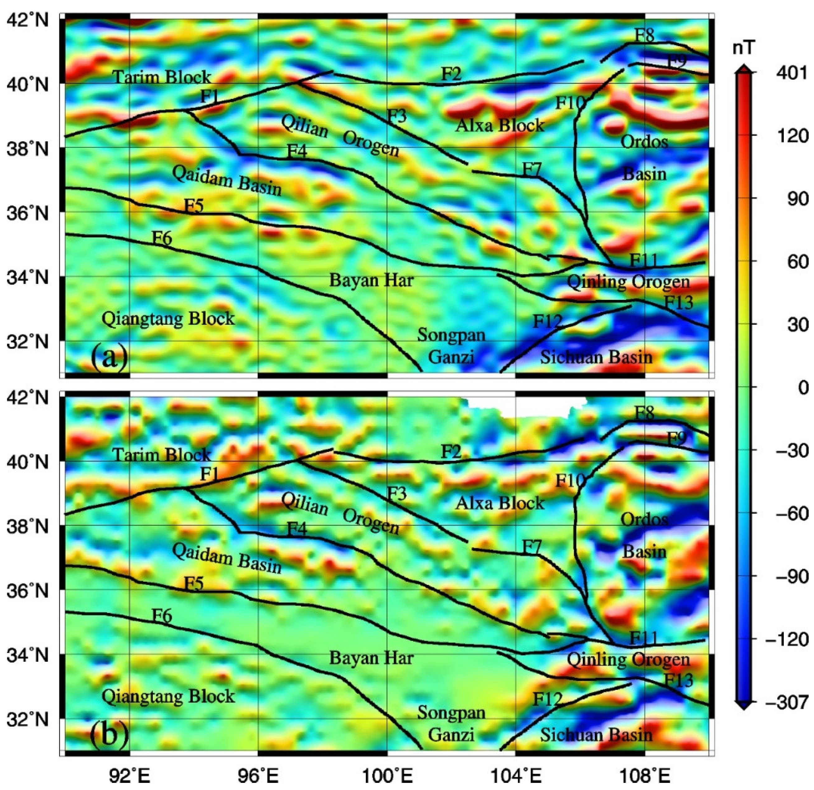
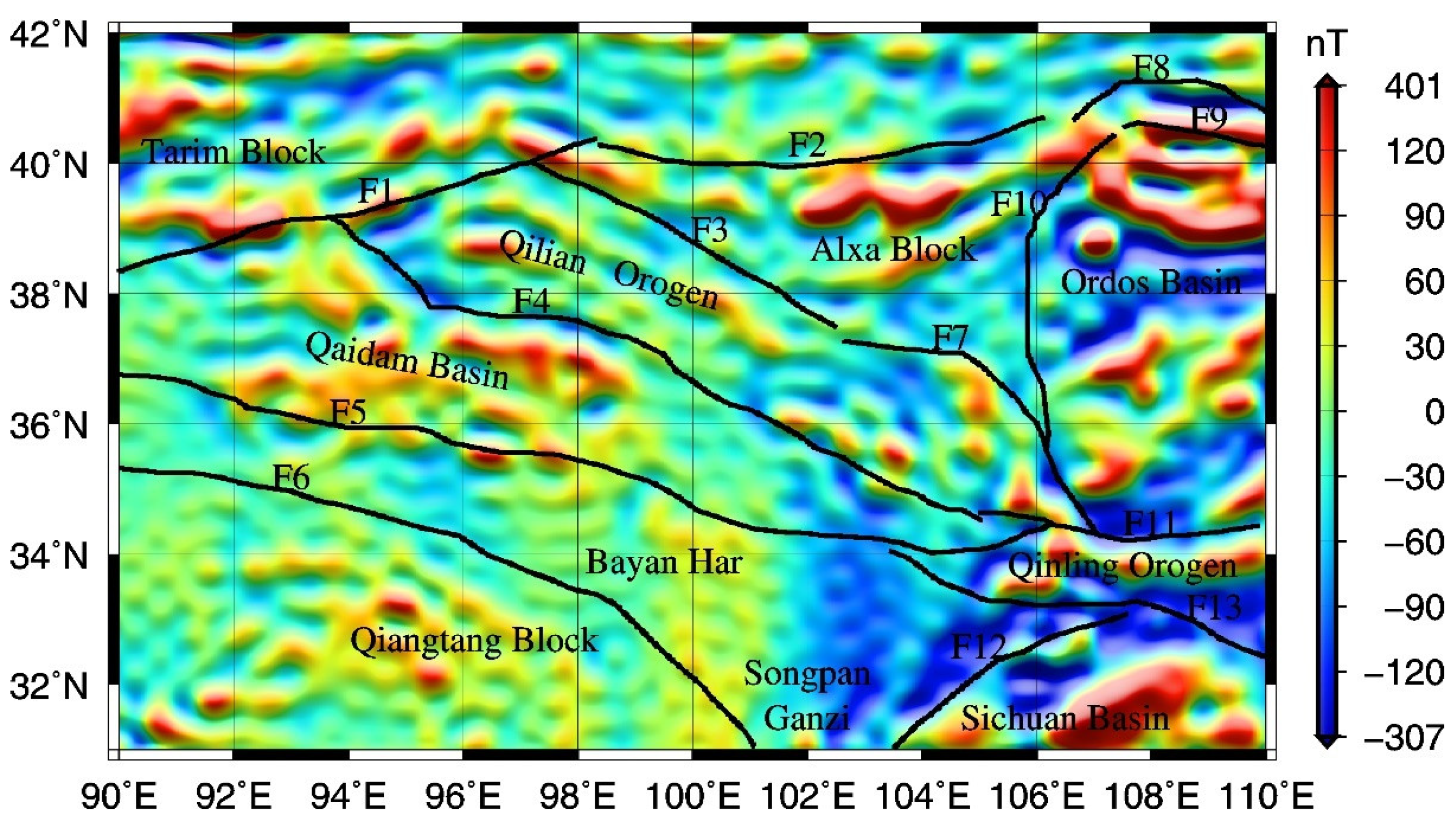
5. Crustal Magnetic Anomalies

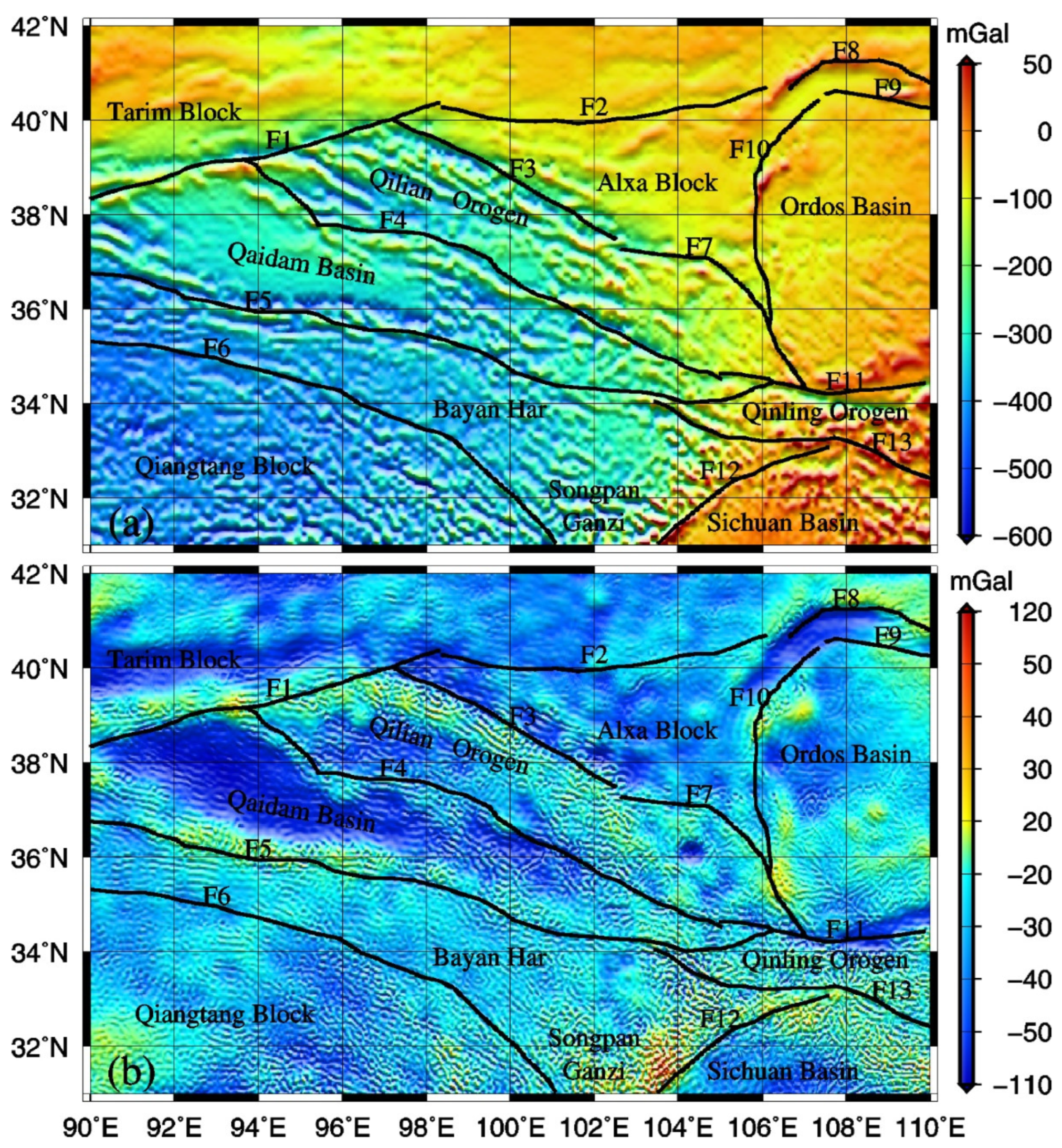
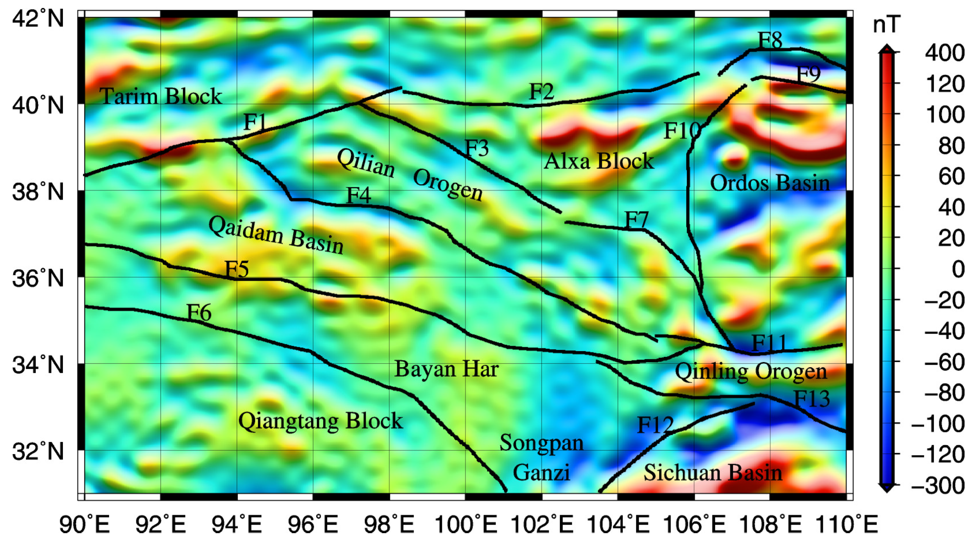
5.1. Crustal Magnetic Anomalies and Aeromagnetic Anomalies

To verify the EMM2017 model, we compared the crustal magnetic anomalies with aeromagnetic anomalies. According to the 1:1,000,000 Aeromagnetic Anomaly Map of Continental China (AAMCC) for an altitude of 1 km compiled by the China Aero Geophysical Survey and Remote Sensing Center for Land and Resources [29], digitalization and continuation were conducted to obtain the distribution of aeromagnetic anomalies on the ground surface (Figure 4b).

The AAMCC was compiled using data collected over limited areas at variable heights and different times. The survey data were acquired during 1957–2011. The data are susceptible to various sources of errors, such as navigational and/or altimetric mislocation and improper removal of regional and external fields. If a regional field is not properly/consistently removed from individual wavelengths in relation to the survey dimensions, then it is difficult to compile a high-quality map for a large area. Moreover, because aeromagnetic surveys are flown at lower heights, the magnetic fields from surface sources suppress the signals from the deeper crust [30]. This suggests that a well-constructed and statistically validated model (e.g., EMM2017) should perform better in studying deep structures than the aeromagnetic data compiled from various sources [31].

The magnetic anomalies obtained using the EMM2017 model (Figure 4a) are consistent with the aeromagnetic anomalies (Figure 4b). The resolution of the aeromagnetic anomalies is better than that of the magnetic anomalies from EMM2017. However, the aeromagnetic anomaly map is a collage of various magnetic survey data, and, more importantly, the relationship between the aeromagnetic anomalies and the depth of the magnetic source is not clear. In addition, only a single magnetic component (ΔT) is provided by aeromagnetic survey technology. These factors limit the recognition and study of crustal magnetic anomalies. However, the EMM2017 model yields a spherical harmonic series with an internally consistent dataset. This is an ideal method for studying crustal magnetic anomalies, as the distribution of magnetic anomalies can be easily obtained from the ground surface to the height of the satellite [32]. Compared with smaller-scale magnetic anomalies, the study of magnetic anomalies associated with geological structures is based on the distribution of larger-scale magnetic anomalies and the magnetic characteristics of various geological units. Therefore, the resolution of the EMM2017 model is sufficient for an analysis of the characteristics of magnetic anomalies and their geological significance in the NETP and adjacent areas.

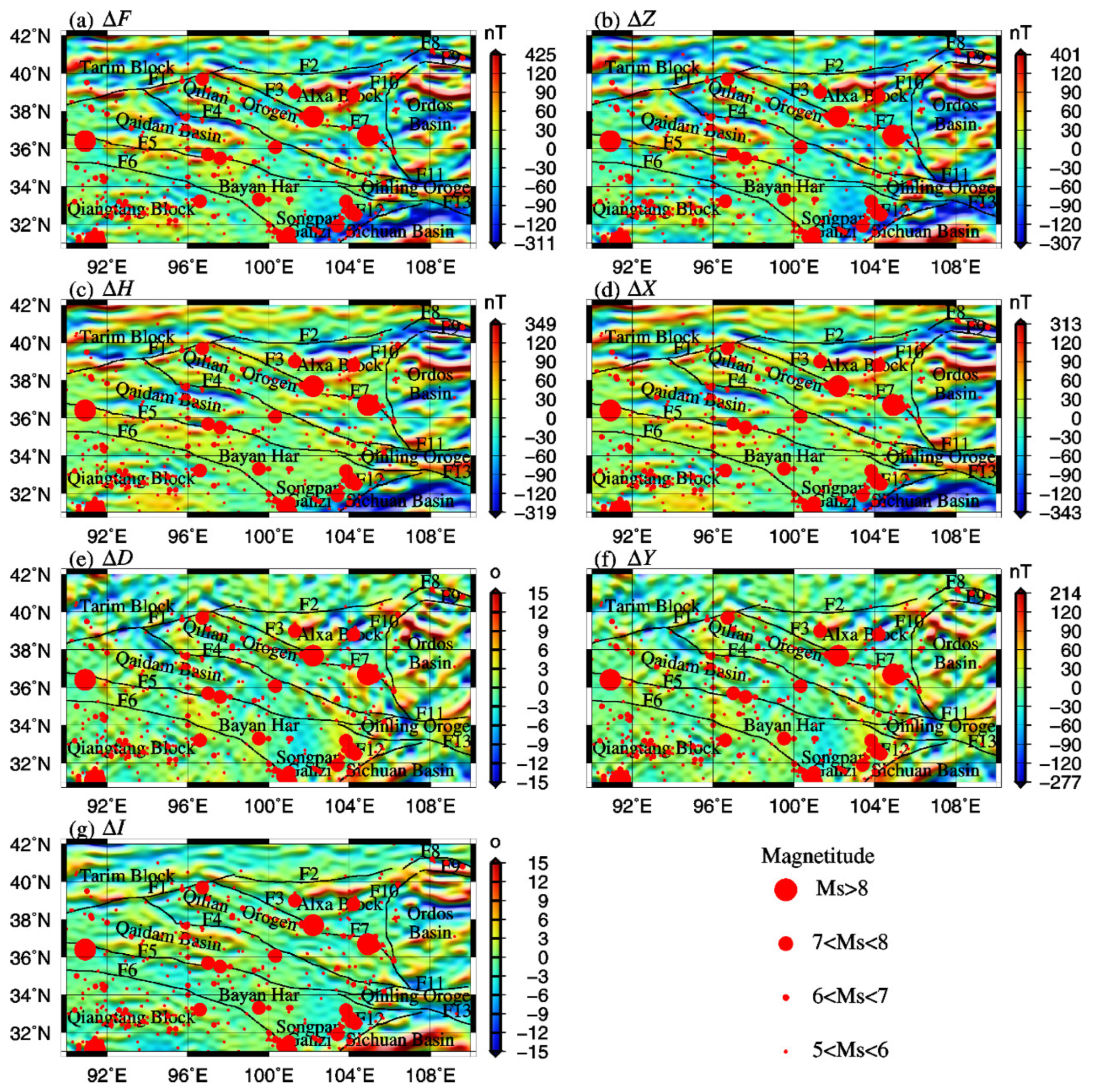
5.2. Distribution of Crustal Magnetic Anomalies

The location of a magnetic anomaly can change due to the effects of inclined magnetization. This leads to challenges in determining the location, morphology, and distribution of a magnetic geological unit and, thus, can affect the interpretation of magnetic anomalies. Therefore, it is necessary to conduct reduction-to-the-pole (RTP) calculations for magnetic anomalies to convert inclined to perpendicular magnetization. The technique of differential RTP with a variable inclination angle was used to conduct RTP calculations for the region considered in this study [33]. Figure 5 shows the RTP magnetic anomaly diagrams of the total intensity ΔF on the ground surface. A comparison between the magnetic anomaly map (Figure 4a) and RTP magnetic map (Figure 5) shows a shift in Figure 5 to the north relative to Figure 4a. The shapes of the magnetic anomalies are also slightly altered because the effects of the inclination and declination of the magnetic field were removed. In the following, we focus on the features of the magnetic anomalies after RTP.

As shown in Figure 5, the magnetic anomalies with different strikes and intensities in the NETP and adjacent areas reflect diverse geological–structural features. The NETP is dominated by orogenic belts undergoing intense tectonic activity, which correspond to weak/negative magnetic anomalies, while the areas adjacent to the NETP are ancient massifs with stable structures that have strong magnetic anomalies. The NETP is mainly characterized by NW–SE-trending magnetic anomalies and faults, corresponding to the Tethyan–Himalayan tectonic domain. The Ordos Basin, which forms the eastern NETP, is dominated by NE–SW-trending magnetic anomalies, corresponding to the Pacific tectonic domain.

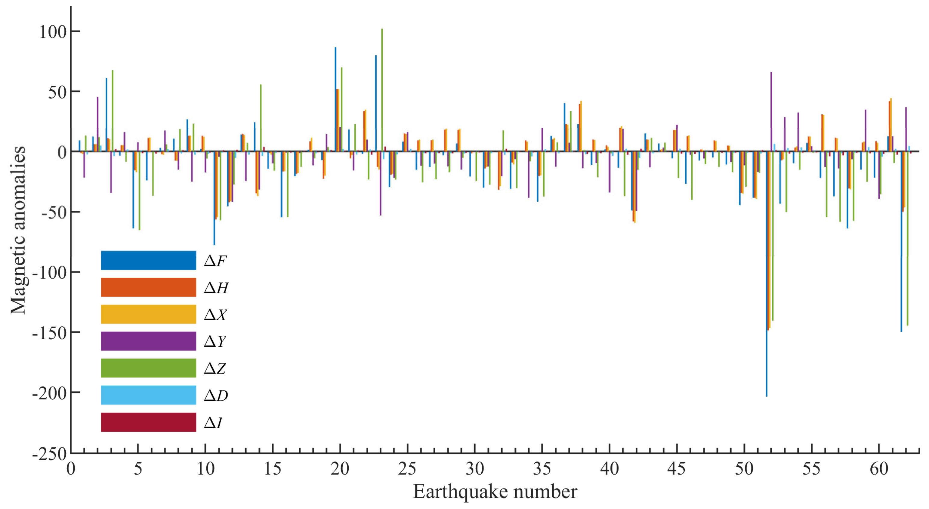
6. Relationships Between the Magnetic Anomalies and Earthquakes

To examine the correlation between the magnetic anomaly distribution and seismic activity, we superimposed the earthquake locations onto the surface magnetic anomaly map (Figure 6). The total intensity ΔF and vertical component ΔZ of the RTP magnetic anomalies are shown in Figure 6a,b, respectively. The earthquake distribution in the study area is mainly concentrated in the NETP and along the main fault zones. The seismic activity varies significantly amongst the different tectonic units. The most frequent seismic activity is in the Qiangtang Block and at the boundary of the Songpan–Ganzi Plateau. There are few earthquakes in the Ordos Block, which is consistent with its stability.

The interior of the Songpan–Ganzi Plateau is dominated by weak and wide negative magnetic anomalies, and the boundary of the plateau is marked by transitions or strong negative magnetic anomalies. Bouguer and isostatic gravity anomalies from WGM2012 are shown in Figure 7 [34]. The isostatic gravity anomalies on most of the NETP are within ±20 mGal, which are considered to indicate a state of gravitational equilibrium. In contrast, gravitational disequilibrium (i.e., positive or negative anomalies) is mostly observed near the boundary zones of blocks and particularly in the Longmen orogenic belt. This belt has an isostatic gravity anomaly as high as 50 mGal, corresponding to a non-isostatic gravity anomaly and the strong tectonic displacement of a deep structure. Most earthquakes occur in the region of the non-isostatic gravity anomalies near the block boundaries, and there is a transition between positive and negative magnetic anomalies or large negative magnetic anomalies.

The Songpan–Ganzi Plateau is adjacent to the West Qinling tectonic belt, Sichuan–Yunnan Block, and Sichuan Basin, and it frequently experiences strong seismic activity. The region is not only the transition zone from the Tibetan Plateau to the Yangtze Platform, but also a convergence zone for material flowing from west to east and from a fast to a slow velocity. The plateau contains a range of geological structures and horizontal displacement velocities (based on GPS observations) as compared with the surrounding blocks (Figure 1). The deep structures also indicate that the plateau is an important gravity anomaly gradient zone and a transition zone where the Mohorovic surface (Moho) shallows abruptly from west to east. The uplift of the Tibetan Plateau as a result of the India–Eurasia collision has led to the eastward flow of deep materials, which are blocked by the rigid Sichuan Basin. Compression, accretion, and lateral flow all occur in the Songpan–Ganzi Plateau. This explains why this area, in which earthquakes occur, is dominated by weak negative magnetic anomalies in its interior, whereas its boundary is a transition zone between positive and negative anomalies or has large negative magnetic anomalies.

Most earthquakes, especially those of Ms ≥ 7, occur along the deep and large faults in the NETP, which mark the boundaries between different blocks. As a result of the India–Eurasia collision, different blocks have variable velocities, leading to stress and energy accumulation at block boundaries. The accumulation of stress can eventually lead to seismicity. This explains why earthquakes of Ms ≥ 7 on the NETP are concentrated along major faults.

In the quantitative analysis of the relationship between the magnetic anomalies and earthquake distribution, we extracted the values of the magnetic anomalies at the epicenters of earthquakes with Ms ≥ 6.0.

Table 2. Focal depths of Ms ≥ 6.0 and corresponding magnetic anomaly values in the study area.

NO.	Date	Lat./(°)	Lon./(°)	Ms	Depth/(km)	ΔF/(nT)	ΔH/(nT)	ΔX/(nT)	ΔY/(nT)	ΔZ/(nT)	ΔD/(°)	ΔI/(°)
Bayan Har Block
1	26 July 1935	33.17	100.94	6.2	15	9.3	−1.2	−2.1	−21.7	13.3	−2.4	0.6
2	7 February 1936	35.44	103.19	6.8	15	12.5	6	6.1	45.4	12	5	0.1
3	7 January 1937	35.43	97.76	7.8	15	61.1	11.1	10.4	−34.2	67.7	−3.8	2
4	17 March 1947	33.48	99.53	7.3	15	−3.4	5.3	5.4	16.1	−8.5	1.7	−0.6
5	5 October 1952	37.01	93.2	6.1	15	−63.8	−15.7	−17.2	7.8	−65.3	0.9	−1.3
6	21 June 1962	36.93	95.93	6.6	17	−23.9	11.4	11.7	0.4	−36.7	−0.2	−1.8
7	19 April 1963	35.61	96.99	6.7	20	3.1	−2.2	−2.8	17.5	5.9	1.9	0.4
8	24 March 1971	35.45	98.14	6	10	10.7	−7.6	−7.7	−15	18.6	−1.7	1.1
9	12 September 2000	35.39	99.34	6.1	10	26.7	13.2	13.2	−25	23.2	−2.8	0.2
10	14 November 2001	35.95	90.54	8.1	10	2.1	13.1	12.2	−17.4	−5.8	−1.9	−0.9
11	17 April 2003	37.53	96.48	6.4	14	−77.8	−56.4	−54.6	−4.4	−57.3	−0.9	1.1
12	28 August 2009	37.7	95.72	6.3	13	−45.5	−42.3	−41.3	−41.8	−27.4	−5.3	1.5
13	21 May 2021	34.6	98.25	7.3	10	14.2	14.6	13.7	−24.5	7.2	−2.6	−0.4
14	28 December 2023	35.7	102.79	6.2	10	24.3	−34.8	−37.1	−31.5	55.7	−3.7	3.9
Qilian Orogen
15	25 December 1920	37.24	105.48	6.8	15	−14.4	−1.2	−2.6	−9.8	−15.9	−1.1	−0.4
16	22 May 1927	37.65	102.49	8	15	−54.6	−16.6	−16.4	−0.9	−54.5	0	−0.9
17	7 March 1928	37.67	102.13	6.2	15	−20.5	−18.6	−18	−1.3	−12.8	0	0.6
18	13 July 1930	37.97	98.26	6.5	10	1.5	8.4	11.5	−11.5	−5.6	−1.5	−0.7
19	25 December 1932	39.5	96.62	7.9	15	−7.1	−22.7	−20	14.5	3.7	1.3	1.2
20	26 December 1951	39.49	95.53	6.2	15	86.7	51.8	51.8	20.4	69.9	2	0.7
21	23 January 1952	39.73	95.44	6	35	18.3	−5.7	−3	−15.8	23	−2.5	1
22	11 February 1954	38.96	101.22	7	25	−2	33.6	34.8	9.9	−23.3	1.7	−2.6
23	31 July 1954	38.62	104.15	6.9	25	79.9	−12.8	−15	−53.1	102.1	−6.3	4.1
24	26 August 1986	37.72	101.5	8.1	8	−29.5	−19.4	−18.6	−22	−23.4	−2.4	0.2
25	14 January 1990	37.82	91.97	6	12	8.2	15	14.5	16.1	0.3	2.1	−0.7
26	26 April 1990	36.05	100.33	6.2	10	−15.1	9.3	10	−11.9	−25.7	−1.3	−1.4
27	26 April 1990	36.24	100.25	6.3	10	−13	9.4	10	−10	−23.1	−1.1	−1.3
28	26 April 1990	36.04	100.27	6.3	10	−3.1	18.2	19	−12.3	−17.2	−1.3	−1.5
29	26 April 1990	35.99	100.25	6.5	8	6.7	18.1	18.9	−15	−5.2	−1.6	−1.1
30	7 January 2022	37.82	101.28	6.6	13	−20.8	−1.5	−0.2	−0.5	−24.6	0.2	−0.8
31	8 January 2022	37.77	101.26	6.9	10	−30	−14.1	−12.9	−12.4	−27.5	−1.3	−0.2
32	26 March 2022	38.5	97.33	6	10	−0.2	−31.9	−28.8	−20.6	17.6	−2.8	2.2
33	16 December 1920	36.89	105.61	8.5	15	−31	−9.2	−10.7	−6.3	−30.4	−0.7	−0.5
Qiangtang Block
34	24 March 1923	31.3	100.75	7	15	−0.2	9.3	8.2	−38.5	−8.2	−4.1	−0.8
35	25 August 1933	32.01	103.68	7.3	15	−41.7	−20.5	−19.8	19.6	−37.5	1.9	−0.7
36	21 August 1950	33.04	91.48	6	15	13	10.1	11.3	−12.6	7.7	−1.4	−0.2
37	28 December 1951	31.06	91.26	7.7	30	40.1	22.8	22.4	7.3	33.7	0.6	0.5
38	26 December 1951	31.24	90.78	6.3	15	22.7	39.4	42.1	−13.8	1.4	−2.2	−2.1
39	14 October 1952	34.35	91.86	6	15	−11.1	10	9.7	−9.6	−21.3	−1.1	−1.4
40	31 October 1952	33.22	101.16	6.2	15	1.8	5.2	3.9	−33.9	−1.5	−3.7	−0.3
41	23 April 1953	31.05	96.87	6	10	−13.5	19.8	21.1	18.9	−37.2	2.2	−2.7
42	4 December 1961	33.34	95.25	6.1	16	−48.9	−58	−59.2	−49.3	−15.2	−5.3	2.3
43	30 August 1967	31.63	100.26	6.4	10	15.1	10.1	9.9	−13.2	11.3	−1.5	0
44	6 February 1973	31.4	100.58	7.4	33	6.7	1.5	1.8	3.3	7.4	0.2	0.3
45	5 May 1975	33.09	92.92	6.1	33	−5.7	17.9	18.1	22.2	−22.1	2.2	−1.8
46	1 January 1977	38.15	91.01	6.3	27	−26.8	12.9	13.4	−2.7	−40.1	−0.1	−2
47	9 June 1981	34.5	91.44	6	10	−7.4	1.7	1.6	−5.8	−10.5	−0.6	−0.5
48	20 August 1986	34.57	91.63	6.4	33	−4.9	9.3	8.8	−0.2	−12.8	0	−1
49	5 November 1988	34.35	91.88	6.2	8	−10.8	5	4.8	−8.7	−17.2	−1	−0.9
50	13 April 2010	33.17	96.55	6.9	17	−44.6	−34.3	−35	−11.5	−29.2	−1.1	0.5
51	14 April 2010	33.2	96.45	6.1	8	−38.5	−38.5	−39.3	−17	−17.8	−1.7	1.2
Songpan−Ganzi Plateau
52	7 February 1958	31.46	104.01	6	25	−203.5	−148.6	−146.6	66	−140.5	6.3	1.2
53	9 November 1960	32.71	103.63	6.3	25	−43.4	−7.3	−6.5	28.5	−50.3	2.9	−1.8
54	11 August 1973	33	104.02	6.1	33	−9.7	3.3	4.2	32.4	−15.1	3.4	−0.9
55	16 August 1976	32.75	104.16	6.9	16	7.1	12.5	12.5	4.5	−1	0.5	−0.8
56	21 August 1976	32.57	104.25	6.4	33	−22	30.9	30.4	−13	−54.5	−1.2	−4
57	23 August 1976	32.49	104.18	6.7	33	−37.3	11.5	11	−14.1	−58.4	−1.4	−3.2
58	22 September 1989	31.58	102.43	6.1	15	−63.9	−30.8	−31.4	−6.4	−57.6	−0.9	−1
59	8 August 2017	33.19	103.86	6.5	9	−15	7.5	8.3	34.8	−25.1	3.7	−1.5
60	10 June 2022	32.25	101.82	6	13	−21.8	8.6	7.3	−39.3	−35.5	−4.3	−2
Ordos Block
61	20 January 1934	41.14	108.62	6.3	15	12.8	41.8	44.4	12.8	−9.5	2.2	−2.6
62	3 May 1996	40.77	109.66	6	26	−149.9	−50.1	−46.4	36.8	−144.6	4.5	−1.7

lists a total of 62 earthquakes of Ms ≥ 6.0, amongst which 50, 8, and 4 earthquakes are of Ms 6, 7, and 8, respectively. The intensity values of the seven elements of the crustal magnetic anomalies at the epicenters are also given in Table 2 and Figure 8.

Table 2 and Figure 6 show that strong earthquakes have occurred mainly in the region where the magnetic anomalies were negative or undergo a strong–weak transition. The proportions of earthquakes in areas with negative magnetic anomalies with geomagnetic elements ΔF, ΔY, ΔZ, ΔI, and ΔD are 63%, 66%, 69%, 65%, and 66%, respectively. Values of ΔX and ΔH are 34 and 26, respectively, in both the positive and negative areas. In general, more earthquakes occur in the areas with negative magnetic anomalies than in the areas with positive anomalies. In terms of the intensity variations of the magnetic anomalies, the extreme positive and negative values of the seven geomagnetic elements (ΔF, ΔH, ΔX, ΔY, ΔZ, ΔD, and ΔI) in the study area are –311 to 425 nT, –319 to 349 nT, –343 to 313 nT, −277 to 214 nT, −307 to 401 nT, −33° to 25°, and −5° to 27°, respectively. In contrast, the magnetic anomalies at the epicenters are much smaller than the extreme values of the positive and negative anomalies. The proportions of earthquakes in areas with negative magnetic anomalies in terms of ΔX and ΔH are not very high. However, combined with the analysis of the intensity of the magnetic anomalies at the epicenters, we conclude that the earthquakes do not occur in areas with extreme positive anomalies but in strong–weak transitional areas near negative magnetic anomalies or the zero contour line. In particular, for the ΔZ component, most earthquakes occur near the zero contour for ΔZ (Figure 6b). The deviation of earthquakes from the zero contour line could be due to uncertainties in the earthquake locations or a failure to fully and accurately separate the crustal magnetic field from the geomagnetic field [16]. The ΔZ gradient may be used to assess the likelihood of seismicity. However, the EMM2017 model only represents the static crustal magnetic field, and such forecasting is only suitable for the medium and long terms.

7. Curie Point Depths

The Curie surface determined by the CPDs is a thermal boundary at which minerals transform from ferromagnetic to paramagnetic, which can provide information on the temperature of the Earth’s interior [21]. Temperature is an important physical parameter of the Earth’s interior because it affects the motion, energy, and stress state of materials. These factors are closely related to the occurrence of earthquakes. Studying the relationship between the Curie surface and seismicity could advance our understanding of the mechanisms of earthquake formation.

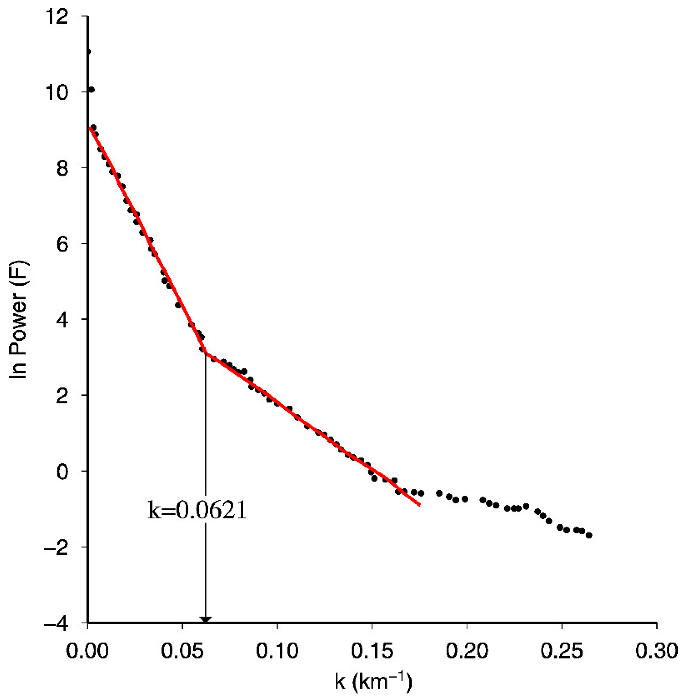
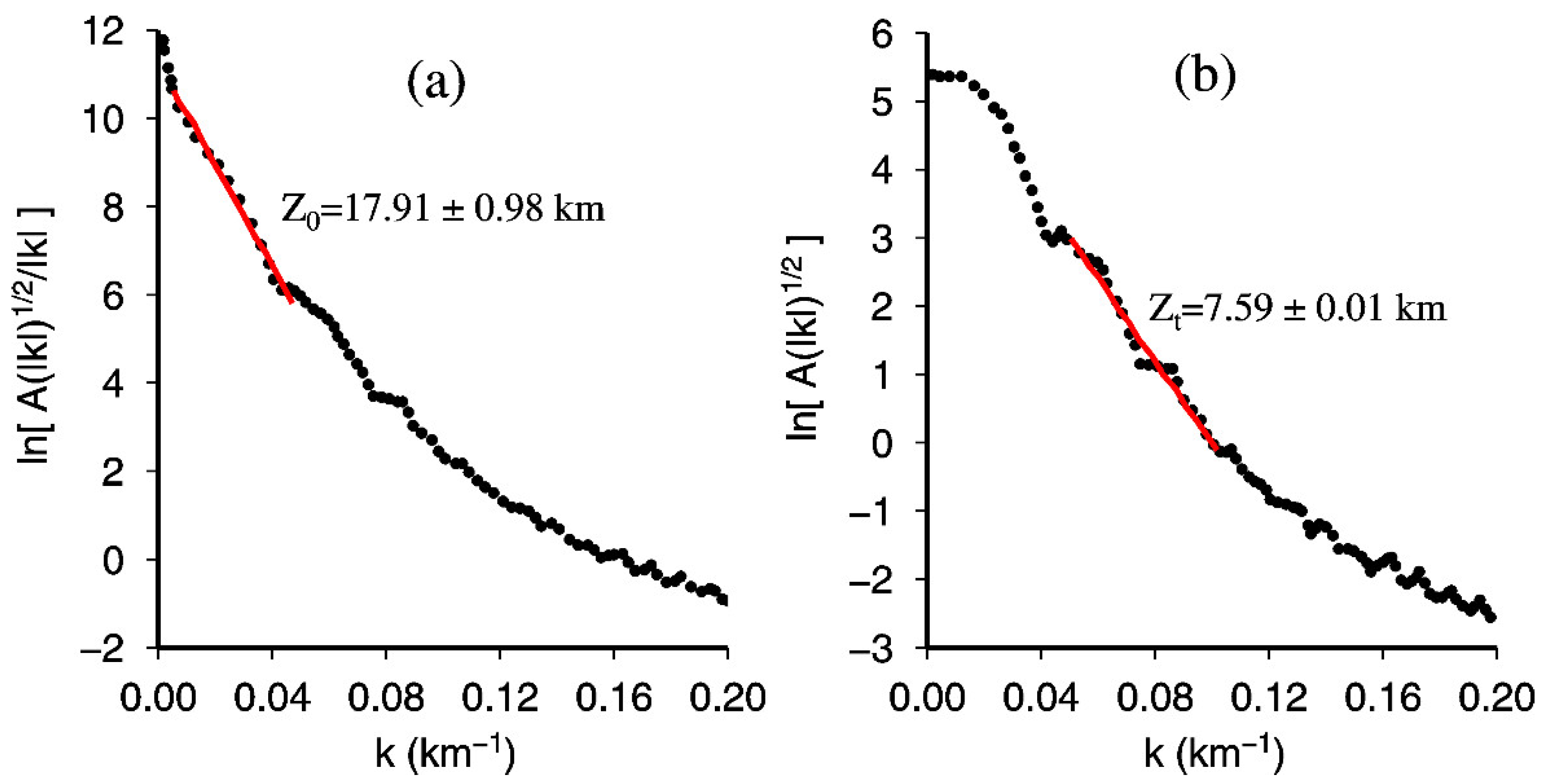
7.1. Calculation of the Curie Point Depth

A magnetic anomaly reflects a combination of effects from shallow and deep crustal magnetic sources [35]. However, the CPD reflects deep magnetic sources. The presence of shallow magnetized bodies tends to reduce the accuracy of the CPD. Therefore, the magnetic anomalies shown in Figure 5 were subjected to low-pass filtering to remove the effects of shallow magnetic sources. Low-pass-filtered magnetic anomalies in the study area (i.e., at a cut-off frequency of 0.0621 km^–1) were obtained from the wavenumber of the shallowest crossing and dipping segments of the power spectra (Figure 9) using the method of Guo and Meng (2013) [36]. Deep magnetized sources are enhanced in the low-pass-filtered magnetic anomaly map of the study region (Figure 10).

In our inversion process, the value of the 3D fractal exponent $\beta$ was 3.0. The magnetic anomaly map in Figure 8 was first divided into a grid of 15 × 8 blocks, each of which had a grid size of 280 × 280 km. To increase the data coverage, all the blocks overlapped with adjoining blocks by 50%. The radially averaged $\ln [A_{\Delta T}{(\left|k\right|)}^{1/2}]$ and $\ln ([A_{\Delta T}{(\left|k\right|)}^{1/2}]/\left|k\right|)$ spectra were then calculated for each block. Finally, the $\ln [A_{\Delta T}{(\left|k\right|)}^{1/2}]$ and $\ln ([A_{\Delta T}{(\left|k\right|)}^{1/2}]/\left|k\right|)$ spectra in the frequency range of 0.0503–0.1017 and 0.0053–0.0471 km⁻¹ were selected to fit Z_t and Z₀, respectively. The CPDs were obtained with Equation (7). Figure 11 shows an example of the fitting of the power spectrum to a block, in which the centroid depth Z₀, the depth with respect to the top of Z_t, and CPD Z_b were 17.91 ± 0.98, 7.59 ± 0.01, and 28.23 ± 2.00 km, respectively.

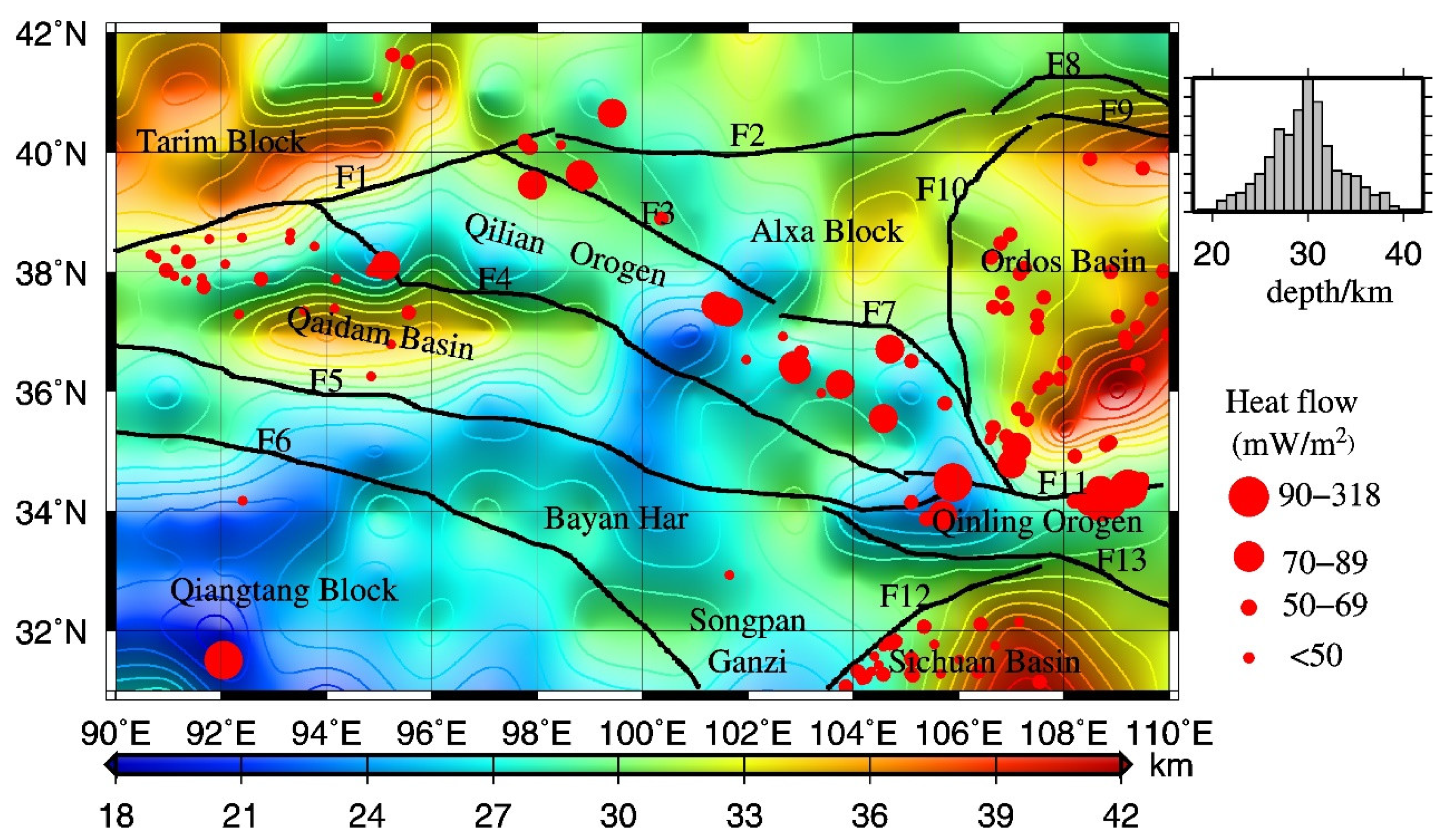
7.2. Distribution of Curie Point Depths

The CPDs in the study area range between 18 and 42 km, with an average of 30 km (Figure 12). This result agrees well with the CPDs obtained from the aeromagnetic surveys. Stable continental regions have a thick magnetic crust, while tectonically active regions are dominated by a thin magnetic crust. The CPDs are deep in the Tarim, Ordos, Qaidam, and Sichuan basins (32–42 km). The deepest CPD is 42 km in the Ordos Basin. The shallowest CPDs (18–30 km) are in the NETP (except for the Qaidam Basin). The shallowest CPD of 18 km is in the Qiangtang Block.

The NETP (except for the Qaidam Basin) is characterized by a shallow CPD due to tectonism. This is consistent with low-velocity layers being ubiquitous in the crust [37] and high heat flows [38]. The high temperature in the NETP crust weakens the crustal magnetism and results in a shallow Curie surface. The Qilian orogenic belt has a shallow Curie surface (CPD = 22–27 km). The crust beneath the orogen is hot and is characterized by intense magmatism, low S-wave velocity anomalies [39], and high heat flow (average = 68 mW/m²) [40]. The Qinling orogenic belt was formed from a continental collision between the North China and South China blocks, and it contains many collision–extrusion-related and extensional detachment structures [41], as well as obvious low-seismic-velocity anomalies [42], which correspond to a shallow CPD (22–27 km). Strong earthquakes (Figure 1) and low S-wave velocity anomalies characterize the Songpan–Ganzi Plateau and Bayan Har Block [42], beneath which the CPD is also shallow (24–27 km).

7.3. Evaluation of Errors in the Curie Point Depth

The errors in the centroid and upper depths of the magnetic sources, ΔZ₀ and ΔZ_t, respectively, were calculated from the slope error on the linear regression [43]. The uncertainty in the depth to the bottom of the magnetic sources (ΔZ_b) was computed using the standard error propagation formula $\Delta Z_b=\sqrt{4\Delta Z_0^2+\Delta Z_t^2}$ [44].

The resulting statistical errors in the centroid and upper depths of the magnetic sources are 0.21–0.95 and 0.01–0.25 km, respectively. The corresponding error in ΔZ_b is 0.4–1.9 km. Errors of similar magnitudes have been obtained in previous studies, such as 0.5–2.1 km in Tanzania [45] and 0.16–2.16 km in Coahuila in Mexico [46].

7.4. Relationship Between the Curie Point Depth and Heat Flow

The thermal gradient was calculated from the CPD data (Z_b) below the ground surface (ΔT) using the Curie–Weiss law, ΔT = (T − T₀)/Z_b [47], assuming the temperature of the ground surface (T₀) is 15 °C and the Curie point (T) is 580 °C. Figure 13 shows the ΔT values in the study area. ΔT varies from 14 to 32 °C/km, with an average of 22 °C/km. The area in which the Curie surface is shallow has a high ΔT, while the area in which the Curie surface is deep has a low ΔT. The ΔT distribution in the study area is similar to that of the CPDs (Figure 12). This indicates that the general trend in the crustal thermal structure can be obtained using ΔT derived from the CPDs.

The CPDs exhibit a correlation with the surface heat flow Qs in the study area. The heat flow data were acquired from the literature [48] and from the Global Heat Flow Database (http://www.heatflow.und.edu/data.html (accessed on 1 January 2025)) (Figure 12). There is a low heat flow in the Tarim, Sichuan, Qaidam, and Ordos basins, with values of 20–70 mW/m², corresponding to CPD values of >30 km. In contrast, the NETP has a high heat flow (>70 mW/m²), corresponding to CPD values of <25 km. The Qiangtang Block has the shallowest CPD (18 km) and a heat flow as high as 318 mW/m².

There is an inverse relationship between the heat flow values and CPDs. We undertook a nonlinear least-squares regression of the data in a plot of the heat flows versus CPDs. Given the study region consists of several blocks with different levels of heat production, we divided it into four blocks: the NETP (mainly the Qinling–Qilian orogenic belt), the Qaidam Basin, the Ordos Basin, and the Sichuan Basin. Using the heat flow data, the CPD values in Figure 12, and Equation 8, we obtained the relationships between these parameters (Figure 14). These results can be used to estimate the heat flow in the study area as follows:

$$Q_s=a{H}^{-b},$$

(8)

where Qs is the heat flow and H is the CPD (in km).

7.5. Correlation Between the Curie Point Depth and Seismicity

The NETP has a relatively shallow CPD, and its crust is tectonically active. Strong earthquakes occur along the geothermal gradient zone where the thermal stress is concentrated. As such, it is possible that the regional seismicity is related to the CPD. Earthquake epicenters are superimposed on the CPD map in Figure 15.

The CPD exhibits an obvious negative correlation with seismic activity. The Curie surface determined from the CPDs is a specific thermal dynamic surface, and its depth shows a good correlation with the background geothermal field and seismicity. Figure 15 shows that earthquakes occur mainly where the Curie surface is shallow or steeply dipping. The earthquakes are mainly observed along the western and northern margins of the Ordos Block, which corresponds to a transition zone between areas with shallow and deep Curie surface. In contrast, there is less seismicity in the interior of the block, corresponding to a relatively uniform and deep CPD. The Alxa Block is relatively stable and has little seismic activity within its interior. However, more seismicity activity is observed at the margin of the block, particularly in the transition zone between the block and Qilian orogenic belt where the Curie surface transitions from shallow to deep. The Curie surface exhibits a depth gradient at the boundaries of the NETP, especially near the Kunlun and Longmenshan faults. Based on the distribution of earthquakes along the fault zones, there is strong coupling between the earthquake distribution and Curie surface.

Most earthquakes in the study area have occurred in the upper crust. Since 1900, there have been 379 earthquakes of Ms ≥ 5.0. The number of earthquakes with a focal depth of <10 km is 273, and the number of earthquakes with a focal depth of 10–20 km is 64, which account for 72% and 17% of all earthquakes, respectively (Figure 16b). Earthquakes with a focal depth of ≤20 km are dominant in the NETP, where the CPD is shallow. Figure 16a shows the focal depths (black dot), the CPDs (blue dotted line), and upper crustal thicknesses (red line) from the global seismic crustal model (Crust 1.0) [49] at the epicenters in Table 1. One can find that most of the focal depths are located in the upper crust. The crustal thermal structure controls the mechanical properties of crustal rocks and variations in rock strength with depth, which define the crustal depth of the brittle–ductile transition and thickness of the seismogenic layer. The crustal temperature of the brittle–ductile transition is generally 300–500 °C [50]. Assuming the temperature of the CPD is 580 °C, the Curie surface is shallower than the upper crust in the NETP (Figure 16a), which indicates that the temperature conditions of the brittle–ductile transition extend into the upper crust beneath the NETP. The rocks in the middle and lower crust do not undergo brittle failure. The NETP is subjected to high stress as a result of India–Eurasia collision and blocking by the rigid Ordos, Sichuan, and Tarim basins, resulting in the middle and lower crusts being unable to withstand a high differential stress or store a large amount of elastic strain energy. As such, the middle and lower crust transfer the tectonic stress to the brittle rocks of the upper crust, resulting in a concentration of differential stress and the accumulation of strain energy. Therefore, earthquakes occur mainly in the upper crust beneath the NETP.

Most earthquakes in the study region have occurred at depths shallower than the CPD (Figure 16a). However, a few earthquakes have occurred at depths greater than the CPD, possibly because these rocks may still be brittle (even at the Curie temperature), which would enable fracturing.

8. Discussion

There are several deep faults around the NETP, and strong earthquakes occur along fault zones. Deep faults are often the boundaries between positive and negative magnetic anomalies, as well as where the Curie surface exhibits a depth gradient. Mantle heat ascends along deep faults, which results in high crustal temperatures and a shallow Curie surface. During the upwelling of crustal material, rocks accumulate strain energy. When the rocks reach the threshold for elastic deformation, the accumulated energy needs to be released, which causes the rocks to fracture, and an earthquake occurs. There is a large difference in the stress in the transition zone across the Curie surface (i.e., the transition between high- and low-temperature zones), which leads to a variable velocity of the material above and below it. As such, energy accumulation due to frictional motion can generate earthquakes.

The Qiangtang Block has a wide, gentle, and low Bouguer gravity anomaly, which reflects a gravity deficit. The heat flow is as high as 318 mW/m² [48], and the block has a very shallow CPD (18 km). In addition, seismic studies have revealed that the Qiangtang Block has a low Q value, low P_n-wave velocity, and only weak S_n waves [51,52]. Lachenbruch (1978) proposed that the high heat flow is due to tectonically induced magmatism [53]. Magmatic additions to the crust in response to extensions might explain the thermal evolution of the Qiangtang Block [54]. The geotherm is heated at depths by upward convection in response to extension and is depressed at shallow levels by rapid sedimentation, thereby maintaining isostatic balance.

Historically, there have been many strong earthquakes in the Qiangtang Block, with 148 earthquakes of Ms ≥ 5.0. Some nearly E–W-trending faults occur around the block, and the fault zones act as channels for magma ascent. The heat flow in this block is as high as 318 mW/m², consistent with the presence of hot springs [48]. During magma upwelling, the pressure and temperature decrease, and the volume of upwelling material increases. Therefore, this process can release energy that causes earthquakes.

The CPDs in the Qilian orogenic belt are different from those in the Qaidam Basin. A deep Curie surface is present in the Qaidam Basin, whereas a shallow Curie surface occurs in the Qilian orogenic belt (Figure 12). The crust of the Qaidam Basin is rigid. Recent seismic and magnetotelluric studies have revealed that the velocity and resistivity are both low beneath the Qilian orogenic belt, while the reverse applies to the Qaidam Basin [55]. The Qilian orogenic belt is in a compressional setting due to the subduction of the Eurasian Plate and the blocking effect of the rigid crust in the Qaidam Basin.

The NETP has negative Bouguer gravity anomalies over a large area (Figure 7a). The low values in this area, coupled with negative/low magnetic anomalies (Figure 5), a shallow Curie surface (Figure 12), and a deep Moho [4], indicate the presence of a hot crust. From the southwest (i.e., the Qiangtang Block) to the northeast (i.e., the Qilian orogenic belt), the gravity anomalies increase and the Moho depth decreases (Figure 7a), which indicates the northeastward expansion of the Tibetan Plateau.

The GPS-derived velocities show that crustal materials from the NETP are moving northeastward (Figure 1). Our study shows that the Tarim, Ordos, and Sichuan basins around the NETP have high gravity values and strong magnetic anomalies (Figure 5), a deep CPD (Figure 12), and shallow Moho [4], indicative of a cold and rigid lithosphere beneath these basins. A shallow CPD corresponds to a low-density crust [56] beneath the NETP, whereas a deep CPD corresponds to a high-density crust beneath its surrounding basins. The subduction of the Indian Plate and blocking by the surrounding rigid basins led to the formation of a lock-in area with a high strain accumulation at the plateau boundaries, which provided the conditions for the formation of low-density and soft materials in the crust beneath the NETP. The northeastern lateral growth of the Tibetan Plateau is due to the blocking effects of the cold and rigid basins.

Clark and Royden (2000) suggested that the large-scale morphology of the Tibetan Plateau can be modeled by eastward fluid flow in the middle to lower crust that is driven by the difference in elevation between the plateau and its surroundings [57]. The eastward flow diverges into southern and northern branches. The southern branch flows around the southwestern side of the Sichuan Basin, while the northern branch appears to be further guided by the strong crust of the Qaidam Basin in the west and flows towards the northeast. Our results for the CPD reveal a northeastward zone from Bayan Har to the Qilian orogenic belt and a deep CPD in the Qaidam Basin (Figure 12) that confirm the northern flow of the plateau.

Our results show that the CPD on the NETP (except for the Qaidam Basin) is shallow (average = 25 km). This indicates that the crustal temperature of the NETP is higher than that of surrounding regions. A study of the three-dimensional lithospheric density structure beneath the Tibetan Plateau [58] revealed that depths of 10–70 km beneath the plateau are dominated by low-density materials. There is a density differential of 0.05 g/cm³ at depths of 10–30 km and 0.1 g/cm³ at depths of 50–70 km between the plateau and surrounding regions. The crust of the plateau is extremely thick, the temperature of the crust is very high, and the density is low (possibly arising from the thermal expansion). As such, the heat source in the interior of the plateau could be a mechanism for the rapid plateau uplift.

9. Conclusions

Earthquakes of Ms ≥ 5.0 have occurred mainly in the tectonically active zone along the NETP and areas where it is connected to surrounding basins. Strong earthquakes occur mainly in areas of negative magnetic anomalies or a strong–weak anomaly transition. Most of these earthquakes occur where the Curie surface is shallow or has a depth gradient. The focal depths of most earthquakes are less than the depth of the Curie surface and are mainly concentrated in the brittle upper crust. The frequent seismic activity in the NETP may be closely related to the northeastward flow of the Tibetan Plateau, which is caused by a deep heat flux. The CPD results show a NE–SW zone from Bayan Har to the Qilian orogenic belt, and the Qaidam Basin with a deep CPD, indicating the northward flow of the Tibetan Plateau. The NETP has shallow CPDs, with an average of 25 km, and a high crustal temperature. The heat source in the plateau’s interior is the main cause of the rapid uplift of the Tibetan Plateau.

Using the EMM2017 model and the observational seismic data to explore the relationships among crustal magnetic anomalies, CPDs, and strong earthquakes is a novel approach. Although the statistical results in this paper are preliminary, they objectively reflect the observed data. Though the physical causes and dynamic process of earthquakes are not well known, we can study the aforementioned relationships that are expected to provide information regarding earthquakes. The study results can be used as a reference for the prediction of strong earthquakes in the region.

References

1. Mavroulis, S.; Mavrouli, M.; Vassilakis, E.; Argyropoulos, I.; Carydis, P.; Lekkas, E. Debris Management in Turkey Provinces Affected by the 6 February 2023 Earthquakes: Challenges during Recovery and Potential Health and Environmental Risks. Appl. Sci. 2023, 13, 8823. [Google Scholar] [CrossRef]
2. Işık, E. Structural Failures of Adobe Buildings during the February 2023 Kahramanmaraş (Türkiye) Earthquakes. Appl. Sci. 2023, 13, 8937. [Google Scholar] [CrossRef]
3. Liu, Y.B.; Pei, S.P. Lower crustal attenuation in northeastern Tibetan Plateau from ML amplitude. Earthq. Sci. 2021, 34, 378–386. [Google Scholar] [CrossRef]
4. Gao, G.M.; Lu, Q.M.; Wang, J.; Kang, G.F. Constraining crustal thickness and lithospheric thermal state beneath the northeastern Tibetan Plateau and adjacent regions from gravity, aeromagnetic, and heat flow data. J. Asian Earth Sci. 2021, 212, 104743. [Google Scholar] [CrossRef]
5. Wang, X.C.; Li, Y.H.; Ding, Z.F.; Zhu, L.P.; Wang, C.Y.; Bao, X.W.; Wu, Y. Three-dimensional lithospheric S wave velocity model of the NE Tibetan Plateau and western North China Craton. J. Geophys. Res. Solid Earth 2017, 122, 6703–6720. [Google Scholar] [CrossRef]
6. Li, Z.; Guo, B.; Liu, Q.Y.; Chen, J.H.; Li, S.C.; Qi, S.H. P-wave structure of upper mantle beneath the Northeastern Tibetan Plateau from multiscale seismic tomography. Chin. J. Geophys. 2019, 62, 1244–1255, (In Chinese with English abstract). [Google Scholar]
7. Xu, W.Y. Physics of Electromagnetic Phenomena of the Earth; University of Science and Technology of China Press: Hefei, China, 2009. [Google Scholar]
8. Gailler, L.S.; Lénat, J.F.; Blakely, R.J. Depth to Curie temperature or bottom of the magnetic sources in the volcanic zone of la Réunion hot spot. J. Volcanol. Geoth. Res. 2016, 324, 169–178. [Google Scholar] [CrossRef]
9. Zu, Q.; Chen, C.H.; Chen, C.R.; Liu, S.; Yen, H.Y. The relationship among earthquake location, magnetization, and subsurface temperature beneath the Taiwan areas. Phys. Earth Planet. Inter. 2021, 320, 106800. [Google Scholar] [CrossRef]
10. Gao, G.M.; Shi, L.; Kang, G.F.; Wu, Y.Y.; Bai, C.H.; Wen, L.W.; Hou, J. Analysis of the lithospheric magnetic anomalies and tectonics in continental China and the adjacent regions using CHAMP satellite data. Stud. Geophys. Geod. 2018, 62, 408–426. [Google Scholar] [CrossRef]
11. Prasad, K.N.D.; Bansal, A.R.; Prakash, O.; Singh, A.P. Magneto-thermometric modeling of Central India: Implications for the thermal lithosphere. J. Appl. Geophys. 2022, 196, 104508. [Google Scholar] [CrossRef]
12. Santos, D.F.; Silva, J.B.C.; Lopes, J.F. In-depth 3D magnetic inversion of basement relief. Geophysics 2022, 87, 45–56. [Google Scholar] [CrossRef]
13. Gao, G.M.; Kang, G.K.; Bai, C.H.; Wen, L.W.; Wang, Z.J.; Li, Y.C. Gravity anomalies and deep structure of the northeastern Tibetan Plateau and adjacent areas. J. Asian Earth Sci. 2025, 278, 106430. [Google Scholar] [CrossRef]
14. Okubo, Y.; Yamano, S.; Takanashi, K.; Akazawa, S.; Osato, K.; Terai, A. Constraining the geotherm beneath the Japanese islands from Curie point depth analysis and comparison with seismicity and drillhole data in the Kakkonda geothermal field. Geothermics 2023, 111, 102706. [Google Scholar] [CrossRef]
15. Wei, R.Q.; Yu, L. Constraints from satellite crustal magnetic field on the distribution of the epicenters for earthquakes in the continental crust of China. Chin. J. Geophys. 2012, 55, 2643–2650, (In Chinese with English abstract). [Google Scholar]
16. Yan, Y.F.; Teng, J.W.; Ruan, X.M.; Hu, G.Z. Aeromagnetic field characteristics and the Wenchuan earthquakes in the Longmenshan mountains and adjacent areas. Chin. J. Geophys. 2016, 59, 197–214, (In Chinese with English abstract). [Google Scholar]
17. Wen, L.M.; Kang, G.F.; Bai, C.H.; Gao, G.M. Relationship between crustal magnetic anomalies and strong earthquake activity in the south segment of the China North-South Seismic Belt. Appl. Geophys. 2021, 18, 408–419. [Google Scholar] [CrossRef]
18. Gao, G.M.; Kang, G.F.; Li, G.Q.; Bai, C.H. Crustal magnetic anomaly in the Ordos region and its tectonic implications. J. Asian Earth Sci. 2015, 109, 63–73. [Google Scholar] [CrossRef]
19. Hamed, S.; Nabi, A.E. Curie point depth beneath the Barramiya-Red Sea coast area estimated from spectral analysis of aeromagnetic data. J. Asian Earth Sci. 2012, 43, 254–266. [Google Scholar]
20. Saada, A.S. Curie point depth and heat flow from spectral analysis of aeromagnetic data over the northern part of Western Desert, Egypt. J. Appl. Geophys. 2016, 134, 100–111. [Google Scholar] [CrossRef]
21. Trifonova, P.; Zhelev, Z.; Petrova, T.; Bojadgieva, K. Curie point depths of Bulgarian territory inferred from geomagnetic observations and its correlation with regional thermal structure and seismicity. Tectonophysics 2009, 473, 362–374. [Google Scholar] [CrossRef]
22. Maus, S. An ellipsoidal harmonic representation of Earth’s lithospheric magnetic field to degree and order 720. Geochem. Geophys. Geosyst. 2010, 11, 1–12. [Google Scholar] [CrossRef]
23. Maus, S.; Rother, M.; Stolle, C.; Mai, W.; Choi, S.; Lühr, H.; Cooke, D.; Roth, C. Third generation of the Potsdam magnetic model of the Earth (POMME). Geochem. Geophys. Geosyst. 2006, 7, Q07008. [Google Scholar] [CrossRef]
24. Olsen, N.; Davat, D.; Finlay, C.C. LCS-1: A high-resolution global model of the lithospheric magnetic field derived from CHAMP and Swarm satellite observations. Geophys. J. Int. 2017, 211, 1461–1477. [Google Scholar] [CrossRef]
25. Meyer, B.; Chulliat, A.; Saltus, R. Derivation and error analysis of the earth magnetic anomaly grid at 2 arc min resolution version 3 (EMAG2v3). Geochem. Geophys. Geosyst. 2017, 18, 4522–4537. [Google Scholar] [CrossRef]
26. Yin, A.; Harrison, T.M. Geologic evolution of the Himalayan-Tibetan orogen. Annu. Rev. Earth planet. Sci. 2000, 28, 211–280. [Google Scholar] [CrossRef]
27. Zhang, P.; Shen, Z.; Wang, M. Continuous deformation of the Tibetan plateau from global positioning system data. Geology 2004, 32, 809–812. [Google Scholar] [CrossRef]
28. Tanaka, A.; Okubo, Y.; Matsubayashi, O. Curie point depth based on spectrum analysis of the magnetic anomalies data in East and Southeast Asia. Tectonophysics 1999, 306, 461–470. [Google Scholar] [CrossRef]
29. Xiong, S.Q.; Yang, H.; Ding, Y.Y.; Li, Z.K. Characteristics of Chinese continent Curie point isotherm. Chin. J. Geophys. 2016, 59, 3604–3617, (In Chinese with English abstract). [Google Scholar]
30. Shive, P.N.; Blakely, R.J.; Fountain, D.M. Magnetic Properties of the lower continental crust. In Continental Lower Crust, Development in Geotectonics; Fountain, D.M., Arculis, R., Kay, R.W., Eds.; Elsevier: Amsterdam, The Netherlands, 1992; Volume 23, pp. 145–199. [Google Scholar]
31. Arnaiz-Rodríguez, M.S.; Orihuela, N. Curie point depth in Venezuela and the Eastern Caribbean. Tectonophysics 2013, 590, 38–51. [Google Scholar] [CrossRef]
32. Kang, G.F.; Gao, G.M.; Bai, C.H.; Shao, D.; Feng, L.L. Characteristics of the crustal magnetic anomaly and regional tectonics in the Qinghai-Tibet Plateau and the adjacent areas. Sci. China Earth Sci. 2011, 41, 1577–1585. [Google Scholar]
33. Cooper, G.R.J.; Cowan, D.R. Differential reduction to the pole. Comput. Geosci. 2005, 31, 989–999. [Google Scholar] [CrossRef]
34. Bonvalot, S.; Balmino, G.; Briais, A.; Kuhn, M.; Peyrefitte, A.; Vales, N.; Biancale, R.; Gabalda, G.; Reinquin, F.; Sarrailh, M. (Eds.) World Gravity Map; Commission for the Geological Map of the World: Paris, France, 2012. [Google Scholar]
35. Thébault, E.; Purucker, M.; Whaler, K.A.; Langlais, B.; Sabaka, T.J. The magnetic field of the earth’s lithosphere. Space Sci. Rev. 2010, 155, 95–127. [Google Scholar] [CrossRef]
36. Guo, L.H.; Meng, X.H. Preferential filtering for gravity anomaly separation. Comput. Geosci. 2013, 51, 247–254. [Google Scholar] [CrossRef]
37. Xia, S.R.; Shi, L.; Li, Y.H. Velocity structures of the crust and uppermost mantal beneath the northeastern margin of Tibetan plateau revealed by double-difference tomography. Chin. J Geophys. 2021, 64, 3194–3206, (In Chinese with English abstract). [Google Scholar]
38. Lysak, S.V. Thermal history, geodynamics, and current thermal activity of lithosphere in China. Russ. Geol. Geophys. 2009, 50, 815–825. [Google Scholar] [CrossRef]
39. Fu, Y.Y.; Xiao, Z. Ambient nois tomography of Rayleigh and Love wave in North Tibetan and adjacent regions. Chin. J. Geophys. 2020, 63, 860–870, (In Chinese with English abstract). [Google Scholar]
40. Hu, S.B.; He, L.; Wang, J. Compilation of heat flow data in the China continental area (3rd ed.). Chin. J. Geophys. 2001, 44, 611–626, (In Chinese with English abstract). [Google Scholar]
41. Wang, C.Y.; Li, Y.H.; Lou, H. Issues on crustal and upper-mantle structures associated with geodynamics in the northeastern Tibetan Plateau. Chin. Sci. Bull. 2016, 61, 2239–2263. [Google Scholar]
42. Ding, W.X.; Fu, Y.Y.; Gao, Y.; Liao, W.L.; He, Y.J.; Cai, Y.J.; Shen, X.L. Phase velocity tomography of Rayleigh in Qinling-Dabie and adjacent areas using ambient seismic noise. Chin. J. Geophys. 2017, 60, 2959–2968, (In Chinese with English abstract). [Google Scholar]
43. Kelemework, Y.; Fedi, M.; Milano, M. A review of spectral analysis of magnetic data for depth estimation. Geophysics 2021, 86, J33. [Google Scholar] [CrossRef]
44. Martos, Y.M.; Catalán, M.; Galindo-Zaldivar, J. Curie depth, heat flux, and thermal subsidence reveal the Pacific mantle outflow through the Scotia Sea. J. Geophys. Res. Solid Earth 2019, 124, 10735–10751. [Google Scholar] [CrossRef]
45. Didas, M.; Armadillo, E.; Hersir, G.; Cumming, W.; Rizzello, D. Regional thermal anomalies derived from magnetic spectral analysis and 3d gravity inversion: Implications for potential geothermal sites in Tanzania. Geothermics 2022, 103, 102431. [Google Scholar] [CrossRef]
46. Carrillo-de la Cruz, J.L.; Prol-Ledesma, R.M.; Gomez-Rodríguez, D.; Rodríguez-Díaz, A. Analysis of the relation between bottom hole temperature data and Curie temperature depth to calculate geothermal gradient and heat flow in Coahuila. Mexico. Tectonophysics 2020, 780, 228397. [Google Scholar] [CrossRef]
47. Saibi, H.; Aboud, E.; Gottsmann, J. Curie point depth from spectral analysis of aeromagnetic data for geothermal reconnaissance in Afghanistan. J. Afr. Earth Sci. 2015, 111, 92–99. [Google Scholar] [CrossRef]
48. Jiang, G.Z.; Gao, P.; Rao, S.; Zhang, L.Y.; Tang, R.Y.; Huang, F.; Zhao, P.; Pang, Z.H.; He, L.J.; Hu, S.B.; et al. Compilation of heat flow data in the continental area of China (4th ed.). Chinese J. Geophys. 2016, 59, 2892–2910, (In Chinese with English Abstract). [Google Scholar]
49. Laske, G.; Masters, G.; Ma, Z.; Pasyanos, M. Update on CRUST1.0-A 1-degree global model of earth’s crust. Geophys. Res. Abstr. 2013, 15, 2658. [Google Scholar]
50. Xiang, C.Y.; Zhou, Z.H. Relationship between seismicity and geothermal structure of the lithosphere in Yunnan Provence, China. Earthq. Res. China 2000, 3, 263–272, (In Chinese with English abstract). [Google Scholar]
51. McNamara, D.E.; Owens, T.J.; Walter, W.R. Observations of regional phase propagation across the Tibetan Plateau. J. Geophys. Res. 1995, 100, 22215–22229. [Google Scholar] [CrossRef]
52. Owens, T.J.; Zandt, G. Implications of crustal property variations for models of Tibetan Plateau evolution. Nature 1997, 387, 37–43. [Google Scholar] [CrossRef]
53. Lachenbruch, A.H. Heat flow in the Basin and Range province and thermal effects of tectonic extension. Pure Appl. Geophys. 1978, 117, 34–50. [Google Scholar] [CrossRef]
54. Gehrels, G.E.; Yin, A.; Wang, X.F. Magmatic history of the northeastern Tibetan Plateau. J. Geophys. Res. Solid Earth 2003, 108, 2423. [Google Scholar] [CrossRef]
55. Liang, H.; Gao, R.; Xue, S.; Han, J. Electrical structure of the middle Qilian Shan revealed by 3-D inversion of magnetotelluric data: New insights into the growth and deformation in the Northeastern Tibetan Plateau. Tectonophysics 2020, 789, 228523. [Google Scholar] [CrossRef]
56. Li, H.L.; Fang, J.; Wang, X.S.; Liu, J.; Cui, R.H.; Chen, M. Lithospheric 3-D density structure beneath the Tibetan plateau and adjacent areas derived from joint inversion of satellite gravity and gravity-gradient data. Chin. J. Geophys. 2017, 60, 2469–2479, (In Chinese with English abstract). [Google Scholar]
57. Clark, M.K.; Royden, L.H. Topographic ooze: Building the eastern margin of Tibet by lower crustal flow. Geology 2000, 28, 703–706. [Google Scholar] [CrossRef]
58. Yang, W.C.; Chen, Z.X.; Hou, Z.Z.; Meng, X.H. Crustal density structures around Chinese continent by inversion of satellite gravity data. Acta. Geol. Sin. 2016, 90, 2167–2175. [Google Scholar]
Figure 1. Map of the topographic relief, major faults (black lines), GPS velocity field (blue arrows), and earthquakes (Ms ≥ 5) since 1900 (red circles) in the NETP and adjacent regions. Abbreviations: F1—Altyn Tagh Fault, F2—Badain–Jaran Fault, F3—North Qilian Suture, F4—South Qilian Suture, F5—Kunlun Fault/Suture, F6—Jinsha Suture, F7—Haiyuan Fault, F8—southern margin of the Yinshan Fault, F9—Huanghe Fault, F10—western margin of the Ordos Fault, F11—northern margin of the Qinling Fault, F12—Longmengshan Fault, and F13—southern margin of the Qinling Fault. The inset at the bottom left shows the location of the study area (red box). CAOB = Central Asian Orogenic Belt; TP = Tibetan Plateau; NCC = North China Craton; YB = Yangtze Block; TB = Tarim Block; IP = Indian Plate. The purple arrow indicates direction of the IP motion. The seismic data are from the China Earthquake Networks Center, National Earthquake Data Center, and United States Geological Survey.
Applsci 15 04331 g001
Figure 2. Map showing the geological structure and major faults (black lines) in the NETP and adjacent areas. The Geological data are from the United States Geological Survey (https://catalog.data.gov (accessed on 1 January 2025)).
Applsci 15 04331 g002
Figure 3. Focal depth of earthquakes in the study areas of Ms ≥ 5.0 since 1900: (a) proportion of earthquake occurrence in different focal depth sections; (b) distribution of earthquakes with different magnitudes in focal depth.
Applsci 15 04331 g003
Figure 4. (a) Crustal magnetic anomalies with the total intensity ΔF on the ground surface obtained from the EMM2017 model. (b) Aeromagnetic anomalies on the ground surface. The northern part of Figure 3b is white due to a lack of survey data. For black lines, please see Figure 1. The magnetic anomaly distribution from EMM2017 is consistent with the aeromagnetic anomalies.
Applsci 15 04331 g004
Figure 5. Crustal magnetic anomalies with the total intensity ΔF after reduction to the pole. For black lines, please see Figure 1. A comparison between the magnetic anomaly map (Figure 4a) and RTP magnetic map (Figure 5) shows a shift to the north.
Applsci 15 04331 g005
Figure 6. Distribution of crustal magnetic anomalies and earthquakes since 1900 in the NETP and adjacent areas for (a) ΔF component, (b) ΔZ component, (c) ΔH component, (d) ΔX component, (e) ΔD component, (f) ΔY component, and (g) ΔI component. Strong earthquakes have occurred mainly in regions where the magnetic anomalies were negative or that had a strong–weak transition.
Applsci 15 04331 g006
Figure 7. Gravity anomalies in the NETP and adjacent areas. (a) Bouguer gravity and (b) isostatic gravity anomalies. For black lines, please see Figure 1. The Bouguer gravity anomalies are negative in the NETP but positive in its vicinity, ranging from −600 to 50 mGal. Gravity disequilibrium (positive or negative) is mostly observed near block boundaries, particularly in the Longmen orogenic belt.
Applsci 15 04331 g007
Figure 8. Magnetic anomalies at the epicenter. The earthquake number in the figure is the same as that in Table 2.
Applsci 15 04331 g008
Figure 9. Power spectrum depth estimate of the magnetic anomalies shown in Figure 4. The arrow shows the cut-off frequency of k = 0.0621 km−1 for the low-pass filtering.
Applsci 15 04331 g009
Figure 10. Low-pass-filtered magnetic anomalies in the NETP and adjacent areas. For black lines, please see Figure 1. The deep magnetized sources appear to be enhanced in the filtered data.
Applsci 15 04331 g010
Figure 11. Example of power spectrum analysis for one subregion and linear fitting to estimate (a) Zt and (b) Z0. For this subregion, the centroid depth Z0, the depth with respect to the top of Zt, and CPD Zb are 17.91 ± 0.98, 7.59 ± 0.01, and 28.23 ± 2.00 km, respectively.
Applsci 15 04331 g011
Figure 12. Map of the Curie surface of the NETP and adjacent areas. The red points indicate surface heat flow. For black lines, please see Figure 1. The CPDs in the study area are 18–42 km, with an average of 30 km.
Applsci 15 04331 g012
Figure 13. Map of the thermal gradient (ΔT) and CPD in the study area. For black lines, please see Figure 1. ΔT varies from 14 to 32 °C/km, with an average of 22 °C/km.
Applsci 15 04331 g013
Figure 14. Nonlinear least-squares fit between the heat flow (Qs) and depth of the Curie surface (H) for different geological areas: (a) the NETP (mainly in the Qinling–Qilian orogenic belt), (b) the Qaidam Basin, (c) the Ordos Basin, and (d) the Sichuan Basin.
Applsci 15 04331 g014
Figure 15. Distribution of the CPD and earthquakes in the NETP and adjacent areas. For black lines, please see Figure 1. Earthquakes tend to occur where the Curie surface is shallow or has a marked depth gradient.
Applsci 15 04331 g015
Figure 16. (a) Plot of focal depths for Ms ≥ 5.0 earthquakes versus the CPDs and upper crustal depths at the epicenters in Table 1. (b) Proportions of earthquakes at different depth intervals. Earthquakes with a focal depth of ≤20 km are dominant in the NETP. Most earthquakes in the study area have occurred in the upper crust.
Applsci 15 04331 g016